Exploring smooth-EM algorithm with various priors
Ziang Zhang
2025-07-07
Last updated: 2025-07-08
Checks: 7 0
Knit directory: InferOrder/
This reproducible R Markdown analysis was created with workflowr (version 1.7.1). The Checks tab describes the reproducibility checks that were applied when the results were created. The Past versions tab lists the development history.
Great! Since the R Markdown file has been committed to the Git repository, you know the exact version of the code that produced these results.
Great job! The global environment was empty. Objects defined in the global environment can affect the analysis in your R Markdown file in unknown ways. For reproduciblity it’s best to always run the code in an empty environment.
The command set.seed(20250707) was run prior to running
the code in the R Markdown file. Setting a seed ensures that any results
that rely on randomness, e.g. subsampling or permutations, are
reproducible.
Great job! Recording the operating system, R version, and package versions is critical for reproducibility.
Nice! There were no cached chunks for this analysis, so you can be confident that you successfully produced the results during this run.
Great job! Using relative paths to the files within your workflowr project makes it easier to run your code on other machines.
Great! You are using Git for version control. Tracking code development and connecting the code version to the results is critical for reproducibility.
The results in this page were generated with repository version 9cb2d00. See the Past versions tab to see a history of the changes made to the R Markdown and HTML files.
Note that you need to be careful to ensure that all relevant files for
the analysis have been committed to Git prior to generating the results
(you can use wflow_publish or
wflow_git_commit). workflowr only checks the R Markdown
file, but you know if there are other scripts or data files that it
depends on. Below is the status of the Git repository when the results
were generated:
Ignored files:
    Ignored:    .DS_Store
    Ignored:    .Rhistory
    Ignored:    .Rproj.user/
    Ignored:    analysis/.DS_Store

Untracked files:
    Untracked:  code/general_EM.R
    Untracked:  code/linear_EM.R
    Untracked:  code/ordering_loading.R
    Untracked:  code/plot_ordering.R
    Untracked:  code/prior_precision.R
    Untracked:  code/simulate.R
    Untracked:  data/loading_order/

Unstaged changes:
    Modified:   analysis/_site.yml
Note that any generated files, e.g. HTML, png, CSS, etc., are not included in this status report because it is ok for generated content to have uncommitted changes.
These are the previous versions of the repository in which changes were
made to the R Markdown (analysis/explore_smoothEM.rmd) and
HTML (docs/explore_smoothEM.html) files. If you’ve
configured a remote Git repository (see ?wflow_git_remote),
click on the hyperlinks in the table below to view the files as they
were in that past version.
| File | Version | Author | Date | Message |
|---|---|---|---|---|
| html | 028201f | Ziang Zhang | 2025-07-08 | Build site. |
| Rmd | ccaa320 | Ziang Zhang | 2025-07-07 | workflowr::wflow_publish("analysis/explore_smoothEM.rmd") |
Introduction
In this study, we consider a mixture model with \(K\) components, specified as follows: \[\begin{equation} \label{eq:smooth-EM} \begin{aligned} \boldsymbol{X}_i \mid z_i = k &\sim \mathcal{N}(\boldsymbol{\mu}_k, \boldsymbol{\Sigma}_k) \quad i\in [n], \\ \boldsymbol{U} = (\boldsymbol{\mu}_1, \ldots, \boldsymbol{\mu}_K) &\sim \mathcal{N}(\boldsymbol{0}, \mathbf{Q}^{-1}), \end{aligned} \end{equation}\] where \(\boldsymbol{X}_i \in \mathbb{R}^d\) denotes the observed data, \(z_i \in [K]\) is a latent indicator assigning observation \(i\) to component \(k\), \(\boldsymbol{\mu}_k \in \mathbb{R}^d\) is the mean vector of component \(k\), and \(\boldsymbol{\Sigma}_k \in \mathbb{R}^{d\times d}\) is its covariance matrix.
The prior distribution over the stacked mean vectors \(\boldsymbol{U}\) is multivariate normal with mean zero and precision matrix \(\mathbf{Q}\). This prior can encode smoothness or structural assumptions about how the component means evolve or are ordered (e.g., spatial or temporal constraints across \(k=1,\ldots,K\)).
Rather than using the standard EM algorithm, we employ a smooth-EM approach that incorporates this structured prior over component means. In this framework:
E-step (standard): \[ \gamma_{ik}^{(t)} = \frac{\pi_k^{(t)} \, \mathcal{N}(\boldsymbol{X}_i \mid \boldsymbol{\mu}_k^{(t)}, \boldsymbol{\Sigma}_k^{(t)})}{\sum_{j=1}^K \pi_j^{(t)} \, \mathcal{N}(\boldsymbol{X}_i \mid \boldsymbol{\mu}_j^{(t)}, \boldsymbol{\Sigma}_j^{(t)})}. \]
M-step (incorporating prior): \[ \begin{aligned} \{\pi^{(t+1)}, \mathbf{U}^{(t+1)}, \boldsymbol{\Sigma}^{(t+1)}\} &= \arg\max \, \mathbb{E}_{\gamma^{(t)}}\Big[\log p(\boldsymbol{X}, \mathbf{U}, \mathbf{Z} \mid \pi, \boldsymbol{\Sigma})\Big] \\ &= \arg\max \, \mathbb{E}_{\gamma^{(t)}}\Big[\log p(\boldsymbol{X}, \mathbf{Z} \mid \pi, \mathbf{U}, \boldsymbol{\Sigma}) + \log p(\mathbf{U})\Big] \\ &= \arg\max \, \bigg\{\mathbb{E}_{\gamma^{(t)}}\Big[\log p(\boldsymbol{X}, \mathbf{Z} \mid \pi, \mathbf{U}, \boldsymbol{\Sigma})\Big] - \frac{1}{2} \mathbf{U}^\top \mathbf{Q} \mathbf{U}\bigg\} \\ &= \arg\max \, \left\{ -\frac{1}{2} \sum_{i,k} \gamma_{ik}^{(t)} \|\boldsymbol{X}_i - \boldsymbol{\mu}_k\|^2_{\boldsymbol{\Sigma}_k^{-1}} - \frac{1}{2} \mathbf{U}^\top \mathbf{Q} \mathbf{U}\right\}. \end{aligned} \]
Unlike the standard EM algorithm, which maximizes the likelihood independently over component means, the smooth-EM algorithm performs MAP estimation that considers the prior of \(\boldsymbol{U}\), encouraging ordered or smooth transitions across components indexed by \(k\).
We will now explore how this smooth-EM algorithm behaves under different prior specifications for \(\mathbf{Q}\).
Simulate mixture in 2D
Here, we will simulate a mixture of Gaussians in 2D, for \(n = 500\) observations and \(K = 5\) components.
source("./code/simulate.R")
library(MASS)
library(mvtnorm)
Warning: package 'mvtnorm' was built under R version 4.3.3palette_colors <- rainbow(5)
alpha_colors <- sapply(palette_colors, function(clr) adjustcolor(clr, alpha.f=0.3))
sim <- simulate_mixture(n=500, K = 5, d=2, seed=123, proj_mat = matrix(c(1,-0.6,-0.6,1), nrow = 2, byrow = T))plot(sim$X, col = alpha_colors[sim$z],
pch = 19, cex = 0.5,
xlab = "X1", ylab = "X2",
main = "Simulated mixture of Gaussians in 2D")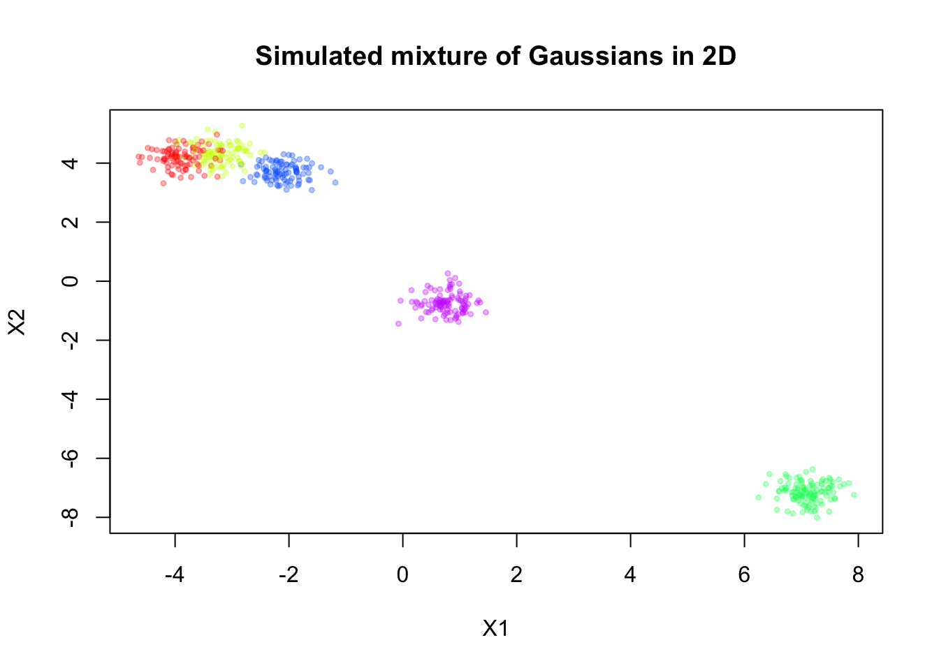
| Version | Author | Date |
|---|---|---|
| 028201f | Ziang Zhang | 2025-07-08 |
Now, let’s assume we don’t know there are five components, and we will fit a mixture model with \(K = 20\) components to this data. For simplicity, let’s assume \(\mathbf{\Sigma}_k = \sigma^2 \mathbf{I}\) for all \(k\), where \(\sigma^2\) is a constant variance across components.
Fitting regular EM
First, we fit the standard EM algorithm to this mixture model without any prior on the means.
library(mclust)Package 'mclust' version 6.1.1
Type 'citation("mclust")' for citing this R package in publications.
Attaching package: 'mclust'The following object is masked from 'package:mvtnorm':
dmvnormfit_mclust <- Mclust(sim$X, G=20)plot(sim$X, col=alpha_colors[sim$z],
xlab="X1", ylab="X2",
cex=0.5, pch=19, main="mclust")
mclust_means <- t(fit_mclust$parameters$mean)
points(mclust_means, pch=3, cex=2, lwd=2, col="red")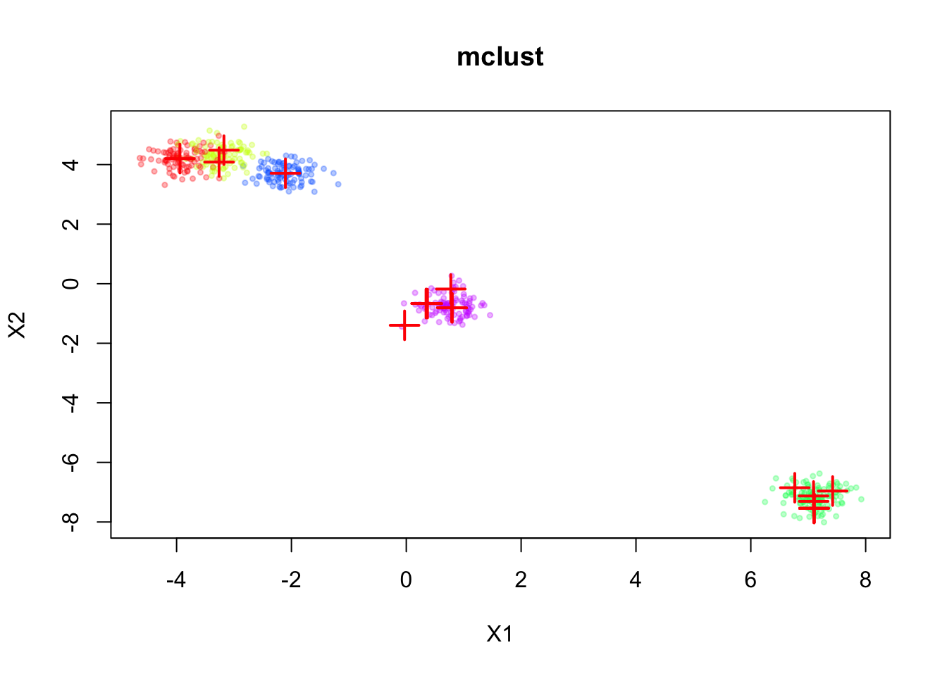
| Version | Author | Date |
|---|---|---|
| 028201f | Ziang Zhang | 2025-07-08 |
The inferred means are shown in red. We can see that the means are well aligned with the true component means, but we don’t have a natural ordering of the means.
Fitting smooth-EM with a linear prior
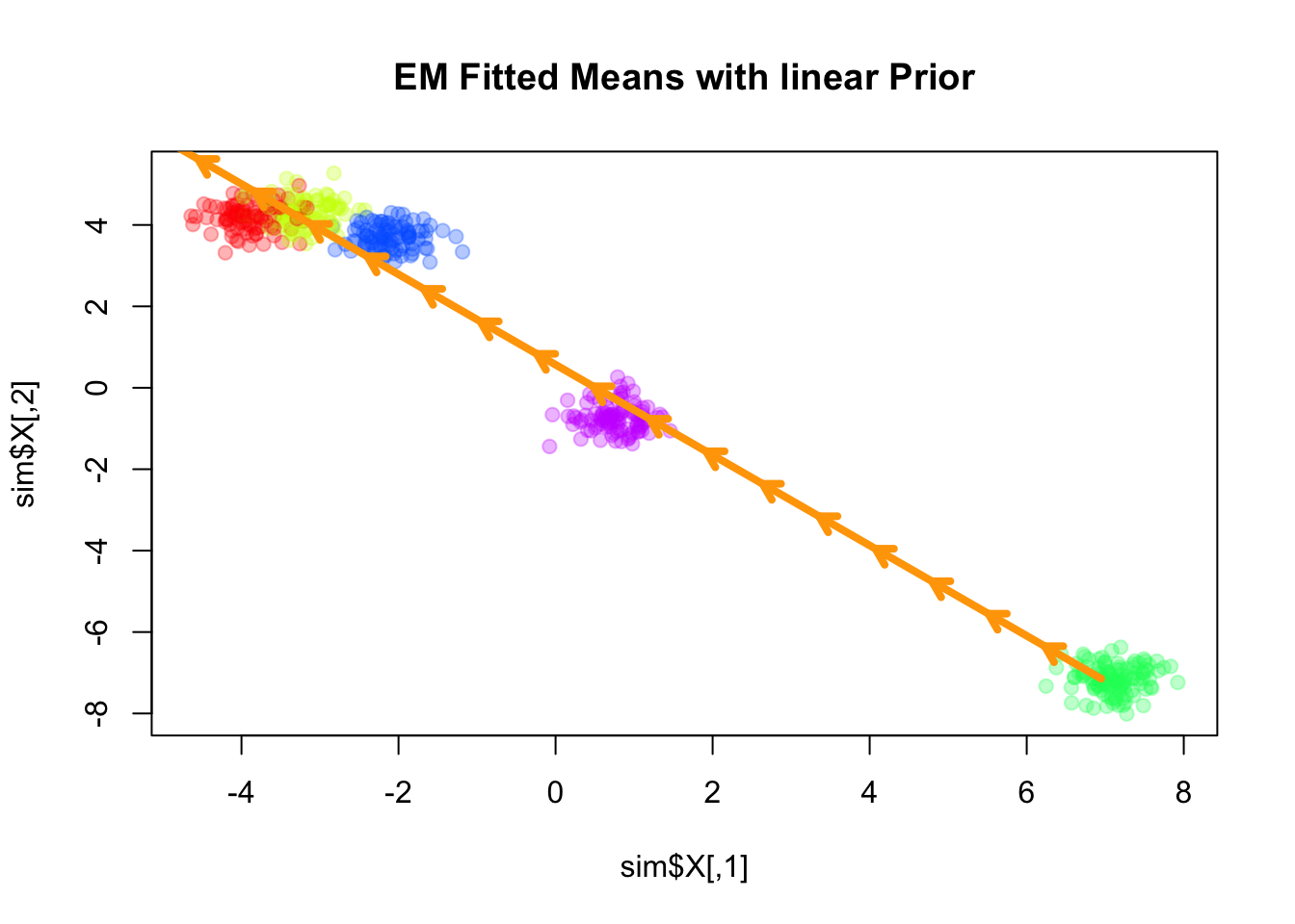
We consider the simplest case for the prior on the component means \(\mathbf{U}\), where \(\mathbf{Q}\) corresponds to a linear trend prior. Specifically, we assume that \[ \boldsymbol{\mu}_k = l_k \boldsymbol{\beta}, \] for some shared slope vector \(\boldsymbol{\beta} \in \mathbb{R}^d\), with \(\{l_k\}\) being equally spaced values increasing from \(-1\) to \(1\).
source("./code/linear_EM.R")
source("./code/general_EM.R")
result_linear <- EM_algorithm_linear(
  data = sim$X,
  K = 20,
  betaprec = 0.001,
  seed = 1,
  max_iter = 50,
  verbose = TRUE
)
Iteration 1: objective = -1794.7853
Iteration 2: objective = -1676.2876
Iteration 3: objective = -1594.5349
Iteration 4: objective = -1547.8152
Iteration 5: objective = -1520.2842
Iteration 6: objective = -1505.5358
Iteration 7: objective = -1499.8317
Iteration 8: objective = -1492.4868
Iteration 9: objective = -1467.2818
Iteration 10: objective = -1423.9226
Iteration 11: objective = -1392.9555
Iteration 12: objective = -1374.1377
Iteration 13: objective = -1362.2392
Iteration 14: objective = -1354.3459
Iteration 15: objective = -1348.9679
Iteration 16: objective = -1345.3093
Iteration 17: objective = -1342.8194
Iteration 18: objective = -1341.0639
Iteration 19: objective = -1339.5998
Iteration 20: objective = -1338.0734
Iteration 21: objective = -1336.8028
Iteration 22: objective = -1335.8233
Iteration 23: objective = -1334.5093
Iteration 24: objective = -1332.5224
Iteration 25: objective = -1329.2927
Iteration 26: objective = -1323.4099
Iteration 27: objective = -1315.5661
Iteration 28: objective = -1303.0675
Iteration 29: objective = -1285.8832
Iteration 30: objective = -1266.5206
Iteration 31: objective = -1242.8967
Iteration 32: objective = -1218.7509
Iteration 33: objective = -1195.0327
Iteration 34: objective = -1174.0646
Iteration 35: objective = -1159.2524
Iteration 36: objective = -1146.8193
Iteration 37: objective = -1139.7610
Iteration 38: objective = -1134.5438
Iteration 39: objective = -1132.4566
Iteration 40: objective = -1130.8451
Iteration 41: objective = -1129.0080
Iteration 42: objective = -1126.3299
Iteration 43: objective = -1123.5453
Iteration 44: objective = -1121.8575
Iteration 45: objective = -1120.8312
Iteration 46: objective = -1120.2198
Iteration 47: objective = -1119.8442
Iteration 48: objective = -1119.5346
Iteration 49: objective = -1119.2344
Iteration 50: objective = -1118.9122plot(sim$X, col=alpha_colors[sim$z], cex=1,
pch=19, main="EM Fitted Means with linear Prior")
# Turn mu_list into matrix
mu_matrix <- do.call(rbind, result_linear$params$mu)
# Draw arrows showing sequence
for (k in 1:(nrow(mu_matrix)-1)) {
arrows(mu_matrix[k,1], mu_matrix[k,2],
mu_matrix[k+1,1], mu_matrix[k+1,2],
col="orange", lwd=4, length=0.1)
}
| Version | Author | Date |
|---|---|---|
| 028201f | Ziang Zhang | 2025-07-08 |
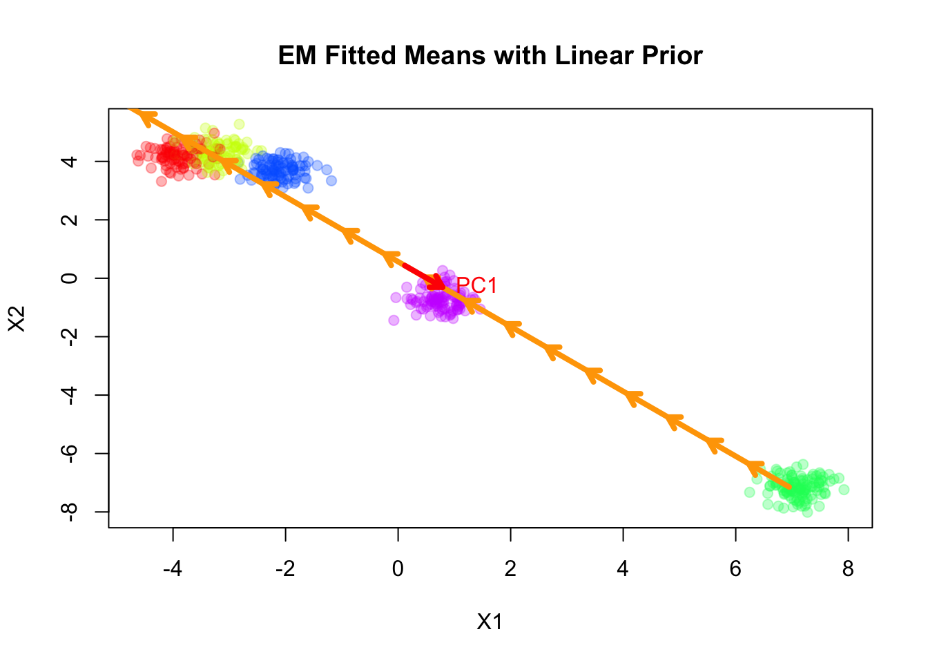
Here the fitted means are shown as orange arrows, with direction indicating the order of the components.
Note that the fitted slope \(\boldsymbol{\beta}\) is very close to the first principal component of the data.
plot(sim$X, col=alpha_colors[sim$z], cex=1,
     xlab="X1", ylab="X2",
     pch=19, main="EM Fitted Means with Linear Prior")

# Turn mu_list into matrix
mu_matrix <- do.call(rbind, result_linear$params$mu)

# Draw arrows showing sequence of cluster means
for (k in 1:(nrow(mu_matrix)-1)) {
  if (sqrt(sum((mu_matrix[k+1,] - mu_matrix[k,])^2)) > 1e-6) {
    arrows(mu_matrix[k,1], mu_matrix[k,2],
           mu_matrix[k+1,1], mu_matrix[k+1,2],
           col="orange", lwd=4, length=0.1)
  }
}

# ====== Fit PCA ======
pca_fit <- prcomp(sim$X, center=TRUE, scale.=FALSE)
pcs <- pca_fit$rotation  # columns are PC directions
X_center <- colMeans(sim$X)

# Set radius for arrows
radius <- 1

# ====== Draw PC arrows ======
arrows(
  X_center[1], X_center[2],
  X_center[1] + radius * pcs[1,1],
  X_center[2] + radius * pcs[2,1],
  col="red", lwd=4, length=0.1
)
text(
  X_center[1] + radius * pcs[1,1],
  X_center[2] + radius * pcs[2,1],
  labels="PC1", pos=4, col="red"
)
| Version | Author | Date |
|---|---|---|
| 028201f | Ziang Zhang | 2025-07-08 |
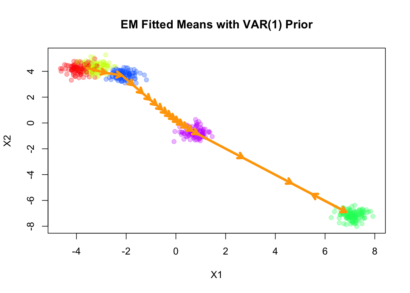
Fitting smooth-EM with a VAR(1) prior
Next, we consider a first-order vector autoregressive (VAR(1)) prior on the component means. Under this prior, each component mean \(\boldsymbol{\mu}_k\) depends linearly on its immediate predecessor \(\boldsymbol{\mu}_{k-1}\), with Gaussian noise: \[ \begin{aligned} \boldsymbol{\mu}_k &= \mathbf{A} \boldsymbol{\mu}_{k-1} + \boldsymbol{\epsilon}_k, \\ \boldsymbol{\epsilon}_k &\sim \mathcal{N}(\mathbf{0}, \mathbf{Q}_\epsilon^{-1}), \end{aligned} \] where \(\mathbf{A}\) is the transition matrix encoding the dependence of the current mean on the previous mean, and \(\mathbf{Q}_\epsilon\) is the precision matrix of the noise term.
Let’s for now assume the transition matrix \(\mathbf{A}\) and the noise precision matrix \(\mathbf{Q}_\epsilon\) are given by:
\[ \mathbf{A} = 0.8 \, \mathbf{I}_2 \] \[ \mathbf{Q}_\epsilon = 0.1 \, \mathbf{I}_2 \]
where \(\mathbf{I}_2\) is the 2-dimensional identity matrix.
source("./code/prior_precision.R")
Q_prior_VAR1 <- make_VAR1_precision(K=20, d=2, A = diag(2) * 0.8, Q = diag(2) * 0.1)
set.seed(1)
init_params <- make_default_init(sim$X, K=20)
result_VAR1 <- EM_algorithm(
  data = sim$X,
  Q_prior = Q_prior_VAR1,
  init_params = init_params,
  max_iter = 50,
  modelName = "EII",
  tol = 1e-5,
  verbose = TRUE
)
Iteration 1: objective = -1958.4957
Iteration 2: objective = -1716.3758
Iteration 3: objective = -1621.1090
Iteration 4: objective = -1483.2038
Iteration 5: objective = -1482.9465
Iteration 6: objective = -1482.7929
Iteration 7: objective = -1482.5235
Iteration 8: objective = -1482.0087
Iteration 9: objective = -1480.9540
Iteration 10: objective = -1478.6996
Iteration 11: objective = -1473.9652
Iteration 12: objective = -1464.8801
Iteration 13: objective = -1449.2401
Iteration 14: objective = -1424.5433
Iteration 15: objective = -1390.0631
Iteration 16: objective = -1350.8749
Iteration 17: objective = -1316.2225
Iteration 18: objective = -1294.2820
Iteration 19: objective = -1286.2432
Iteration 20: objective = -1285.0849
Converged at iteration 21 with objective -1285.3027plot(sim$X, col=alpha_colors[sim$z], cex=1,
xlab="X1", ylab="X2",
pch=19, main="EM Fitted Means with VAR(1) Prior")
# Turn mu_list into matrix
mu_matrix <- do.call(rbind, result_VAR1$params$mu)
# Draw arrows showing sequence of cluster means
for (k in 1:(nrow(mu_matrix)-1)) {
if (sqrt(sum((mu_matrix[k+1,] - mu_matrix[k,])^2)) > 1e-6) {
arrows(mu_matrix[k,1], mu_matrix[k,2],
mu_matrix[k+1,1], mu_matrix[k+1,2],
col="orange", lwd=4, length=0.1)
}
}
| Version | Author | Date |
|---|---|---|
| 028201f | Ziang Zhang | 2025-07-08 |
Fitting smooth-EM with a RW1 prior
Next, we consider a first-order random walk (RW1) prior on the component means, formulated using the difference operator. Under this prior, successive differences of the means are modeled as independent Gaussian noise:
\[ \Delta \boldsymbol{\mu}_k = \boldsymbol{\mu}_k - \boldsymbol{\mu}_{k-1} \sim \mathcal{N}\big(\mathbf{0}, \lambda^{-1} \mathbf{I}_d\big), \]
where \(\lambda\) is a scalar precision parameter that controls the smoothness of the mean sequence. Larger values of \(\lambda\) enforce stronger smoothness by penalizing large differences between successive component means.
Q_prior_RW1 <- make_random_walk_precision(K=20, d=2, lambda = 5)
result_RW1 <- EM_algorithm(
  data = sim$X,
  Q_prior = Q_prior_RW1,
  init_params = init_params,
  max_iter = 50,
  modelName = "EII",
  tol = 1e-5,
  verbose = TRUE
)
Iteration 1: objective = -1669.1600
Iteration 2: objective = -1447.0245
Iteration 3: objective = -1430.4711
Iteration 4: objective = -1417.7644
Iteration 5: objective = -1352.0973
Iteration 6: objective = -1320.7124
Iteration 7: objective = -1320.7116
Iteration 8: objective = -1320.7105
Iteration 9: objective = -1320.7081
Iteration 10: objective = -1320.7029
Iteration 11: objective = -1320.6914
Iteration 12: objective = -1320.6650
Iteration 13: objective = -1320.5996
Iteration 14: objective = -1320.4142
Iteration 15: objective = -1319.7833
Iteration 16: objective = -1317.4450
Iteration 17: objective = -1309.8554
Iteration 18: objective = -1289.4234
Iteration 19: objective = -1244.3649
Iteration 20: objective = -1170.6025
Iteration 21: objective = -1110.6832
Iteration 22: objective = -1097.4406
Iteration 23: objective = -1096.1111
Iteration 24: objective = -1095.8917
Iteration 25: objective = -1095.8366
Iteration 26: objective = -1095.8194
Iteration 27: objective = -1095.8132
Iteration 28: objective = -1095.8107
Iteration 29: objective = -1095.8094
Iteration 30: objective = -1095.8084
Iteration 31: objective = -1095.8075
Iteration 32: objective = -1095.8067
Iteration 33: objective = -1095.8057
Iteration 34: objective = -1095.8046
Iteration 35: objective = -1095.8034
Iteration 36: objective = -1095.8021
Iteration 37: objective = -1095.8006
Iteration 38: objective = -1095.7989
Iteration 39: objective = -1095.7969
Iteration 40: objective = -1095.7947
Iteration 41: objective = -1095.7922
Iteration 42: objective = -1095.7893
Iteration 43: objective = -1095.7860
Iteration 44: objective = -1095.7822
Iteration 45: objective = -1095.7777
Iteration 46: objective = -1095.7726
Iteration 47: objective = -1095.7666
Iteration 48: objective = -1095.7596
Iteration 49: objective = -1095.7514
Iteration 50: objective = -1095.7417plot(sim$X, col=alpha_colors[sim$z], cex=1,
xlab="X1", ylab="X2",
pch=19, main="EM Fitted Means with RW(1) Prior")
# Turn mu_list into matrix
mu_matrix <- do.call(rbind, result_RW1$params$mu)
# Draw arrows showing sequence of cluster means
for (k in 1:(nrow(mu_matrix)-1)) {
if (sqrt(sum((mu_matrix[k+1,] - mu_matrix[k,])^2)) > 1e-6) {
arrows(mu_matrix[k,1], mu_matrix[k,2],
mu_matrix[k+1,1], mu_matrix[k+1,2],
col="orange", lwd=4, length=0.1)
}
}Warning in arrows(mu_matrix[k, 1], mu_matrix[k, 2], mu_matrix[k + 1, 1], :
zero-length arrow is of indeterminate angle and so skipped
Warning in arrows(mu_matrix[k, 1], mu_matrix[k, 2], mu_matrix[k + 1, 1], :
zero-length arrow is of indeterminate angle and so skipped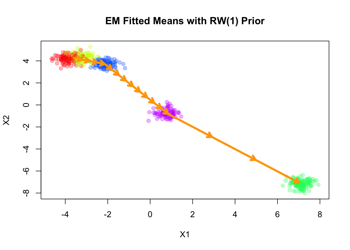
| Version | Author | Date |
|---|---|---|
| 028201f | Ziang Zhang | 2025-07-08 |
The result of RW1 looks similar to that of VAR(1), which is not surprising since the RW1 prior is a special case of the VAR(1) prior with \(\mathbf{A} = \mathbf{I}\).
Note that RW1 is a partially improper prior, as the overall level of the means is not penalized. In other words, the prior is invariant to addition of any constant vector to all component means.
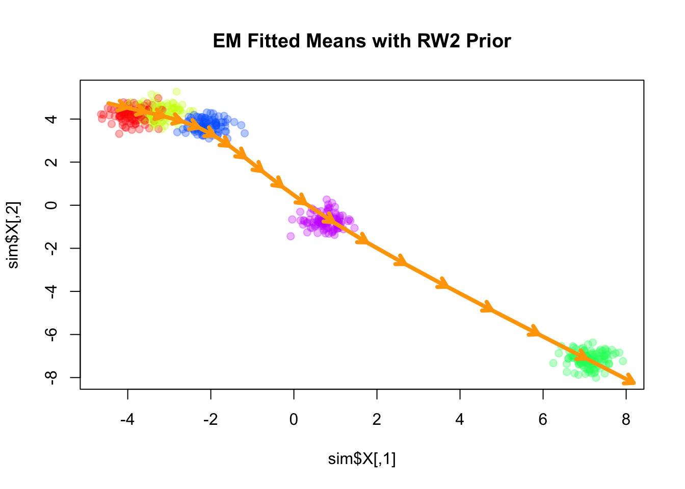
Fitting smooth-EM with a RW2 prior
Next, we consider a second-order random walk (RW2) prior on the component means, which penalizes the second differences of the means:
\[ \Delta^2 \boldsymbol{\mu}_k = \boldsymbol{\mu}_k - 2\boldsymbol{\mu}_{k-1} + \boldsymbol{\mu}_{k-2} \sim \mathcal{N}\big(\mathbf{0}, \lambda^{-1} \mathbf{I}_d\big), \]
where \(\Delta^2 \boldsymbol{\mu}_k\) denotes the second-order difference operator. The scalar precision parameter \(\lambda\) controls the smoothness of the sequence, with larger values enforcing stronger penalization of curvature.
Q_prior_rw2 <- make_random_walk_precision(K = 20, d = 2, q=2, lambda=400)
result_rw2 <- EM_algorithm(
  data = sim$X,
  Q_prior = Q_prior_rw2,
  init_params = init_params,
  max_iter = 50,
  modelName = "EII",
  tol = 1e-5,
  verbose = TRUE
)
Iteration 1: objective = -2717.3131
Iteration 2: objective = -2040.4867
Iteration 3: objective = -1712.1471
Iteration 4: objective = -1626.4376
Iteration 5: objective = -1384.5483
Iteration 6: objective = -1220.9010
Iteration 7: objective = -1198.9225
Iteration 8: objective = -1195.9110
Iteration 9: objective = -1195.2222
Iteration 10: objective = -1194.4981
Iteration 11: objective = -1193.2618
Iteration 12: objective = -1190.6613
Iteration 13: objective = -1184.5477
Iteration 14: objective = -1169.4566
Iteration 15: objective = -1134.6713
Iteration 16: objective = -1076.3360
Iteration 17: objective = -1032.1404
Iteration 18: objective = -1022.9190
Iteration 19: objective = -1022.2435
Iteration 20: objective = -1022.2303
Iteration 21: objective = -1022.1385
Iteration 22: objective = -1021.9050
Iteration 23: objective = -1021.4831
Iteration 24: objective = -1020.7971
Iteration 25: objective = -1019.7545
Iteration 26: objective = -1018.2650
Iteration 27: objective = -1016.2637
Iteration 28: objective = -1013.7339
Iteration 29: objective = -1010.7330
Iteration 30: objective = -1007.4247
Iteration 31: objective = -1004.0931
Iteration 32: objective = -1001.0844
Iteration 33: objective = -998.6681
Iteration 34: objective = -996.9198
Iteration 35: objective = -995.7364
Iteration 36: objective = -994.9474
Iteration 37: objective = -994.4062
Iteration 38: objective = -994.0169
Iteration 39: objective = -993.7237
Iteration 40: objective = -993.4947
Iteration 41: objective = -993.3106
Iteration 42: objective = -993.1591
Iteration 43: objective = -993.0317
Iteration 44: objective = -992.9223
Iteration 45: objective = -992.8264
Iteration 46: objective = -992.7407
Iteration 47: objective = -992.6623
Iteration 48: objective = -992.5895
Iteration 49: objective = -992.5204
Iteration 50: objective = -992.4537plot(sim$X, col=alpha_colors[sim$z], cex=1,
pch=19, main="EM Fitted Means with RW2 Prior")
# Turn mu_list into matrix
mu_matrix <- do.call(rbind, result_rw2$params$mu)
# Draw arrows showing sequence
for (k in 1:(nrow(mu_matrix)-1)) {
arrows(mu_matrix[k,1], mu_matrix[k,2],
mu_matrix[k+1,1], mu_matrix[k+1,2],
col="orange", lwd=4, length=0.1)
}
| Version | Author | Date |
|---|---|---|
| 028201f | Ziang Zhang | 2025-07-08 |
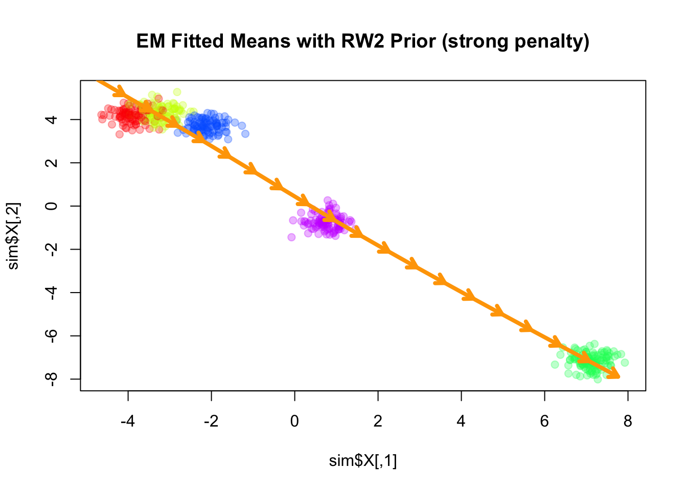
Similar to the RW1 prior, the RW2 prior is also a partially improper prior, as it is invariant to addition of a constant vector as well as a linear trend (in terms of \(k\)) to all component means. As \(\lambda\) increases, the fitted means become closer to a linear trend.
Q_prior_rw2_strong <- make_random_walk_precision(K = 20, d = 2, q=2, lambda=4000)
Q_prior_rw2_strong <- EM_algorithm(
  data = sim$X,
  Q_prior = Q_prior_rw2_strong,
  init_params = init_params,
  max_iter = 50,
  modelName = "EII",
  tol = 1e-5,
  verbose = TRUE
)
Iteration 1: objective = -2543.3091
Iteration 2: objective = -1875.5104
Iteration 3: objective = -1225.2726
Iteration 4: objective = -1180.2106
Iteration 5: objective = -1177.4332
Iteration 6: objective = -1171.3993
Iteration 7: objective = -1159.9830
Iteration 8: objective = -1143.1198
Iteration 9: objective = -1126.1589
Iteration 10: objective = -1114.7535
Iteration 11: objective = -1106.9885
Iteration 12: objective = -1099.3001
Iteration 13: objective = -1090.3622
Iteration 14: objective = -1080.6620
Iteration 15: objective = -1072.0990
Iteration 16: objective = -1066.5441
Iteration 17: objective = -1063.9732
Iteration 18: objective = -1063.0584
Iteration 19: objective = -1062.7694
Iteration 20: objective = -1062.6747
Iteration 21: objective = -1062.6364
Iteration 22: objective = -1062.6116
Iteration 23: objective = -1062.5833
Iteration 24: objective = -1062.5382
Iteration 25: objective = -1062.4584
Iteration 26: objective = -1062.3137
Iteration 27: objective = -1062.0516
Iteration 28: objective = -1061.5820
Iteration 29: objective = -1060.7606
Iteration 30: objective = -1059.3833
Iteration 31: objective = -1057.2288
Iteration 32: objective = -1054.2017
Iteration 33: objective = -1050.5410
Iteration 34: objective = -1046.8627
Iteration 35: objective = -1043.8279
Iteration 36: objective = -1041.7294
Iteration 37: objective = -1040.4537
Iteration 38: objective = -1039.7286
Iteration 39: objective = -1039.3187
Iteration 40: objective = -1039.0764
Iteration 41: objective = -1038.9221
Iteration 42: objective = -1038.8162
Iteration 43: objective = -1038.7395
Iteration 44: objective = -1038.6818
Iteration 45: objective = -1038.6378
Iteration 46: objective = -1038.6039
Iteration 47: objective = -1038.5779
Iteration 48: objective = -1038.5578
Iteration 49: objective = -1038.5424
Iteration 50: objective = -1038.5307plot(sim$X, col=alpha_colors[sim$z], cex=1,
pch=19, main="EM Fitted Means with RW2 Prior (strong penalty)")
# Turn mu_list into matrix
mu_matrix <- do.call(rbind, Q_prior_rw2_strong$params$mu)
# Draw arrows showing sequence
for (k in 1:(nrow(mu_matrix)-1)) {
arrows(mu_matrix[k,1], mu_matrix[k,2],
mu_matrix[k+1,1], mu_matrix[k+1,2],
col="orange", lwd=4, length=0.1)
}
| Version | Author | Date |
|---|---|---|
| 028201f | Ziang Zhang | 2025-07-08 |
sessionInfo()R version 4.3.1 (2023-06-16)
Platform: aarch64-apple-darwin20 (64-bit)
Running under: macOS Monterey 12.7.4
Matrix products: default
BLAS: /Library/Frameworks/R.framework/Versions/4.3-arm64/Resources/lib/libRblas.0.dylib
LAPACK: /Library/Frameworks/R.framework/Versions/4.3-arm64/Resources/lib/libRlapack.dylib; LAPACK version 3.11.0
locale:
[1] en_US.UTF-8/en_US.UTF-8/en_US.UTF-8/C/en_US.UTF-8/en_US.UTF-8
time zone: America/Chicago
tzcode source: internal
attached base packages:
[1] stats graphics grDevices utils datasets methods base
other attached packages:
[1] mclust_6.1.1 mvtnorm_1.3-1 MASS_7.3-60 workflowr_1.7.1
loaded via a namespace (and not attached):
[1] jsonlite_2.0.0 compiler_4.3.1 promises_1.3.3 Rcpp_1.0.14
[5] stringr_1.5.1 git2r_0.33.0 callr_3.7.6 later_1.4.2
[9] jquerylib_0.1.4 yaml_2.3.10 fastmap_1.2.0 R6_2.6.1
[13] knitr_1.50 tibble_3.2.1 rprojroot_2.0.4 bslib_0.9.0
[17] pillar_1.10.2 rlang_1.1.6 cachem_1.1.0 stringi_1.8.7
[21] httpuv_1.6.16 xfun_0.52 getPass_0.2-4 fs_1.6.6
[25] sass_0.4.10 cli_3.6.5 magrittr_2.0.3 ps_1.9.1
[29] digest_0.6.37 processx_3.8.6 rstudioapi_0.16.0 lifecycle_1.0.4
[33] vctrs_0.6.5 evaluate_1.0.3 glue_1.8.0 whisker_0.4.1
[37] rmarkdown_2.28 httr_1.4.7 tools_4.3.1 pkgconfig_2.0.3
[41] htmltools_0.5.8.1