Infering latent ordering from the pancrea dataset

workflowr

• Summary
• Checks
• Past versions

Last updated: 2025-07-09

Checks: 7 0

Knit directory: InferOrder/

This reproducible R Markdown analysis was created with workflowr (version 1.7.1). The Checks tab describes the reproducibility checks that were applied when the results were created. The Past versions tab lists the development history.

---

R Markdown file: up-to-date

Great! Since the R Markdown file has been committed to the Git repository, you know the exact version of the code that produced these results.

Environment: empty

Great job! The global environment was empty. Objects defined in the global environment can affect the analysis in your R Markdown file in unknown ways. For reproduciblity it’s best to always run the code in an empty environment.

Seed: set.seed(20250707)

The command set.seed(20250707) was run prior to running the code in the R Markdown file. Setting a seed ensures that any results that rely on randomness, e.g. subsampling or permutations, are reproducible.

Session information: recorded

Great job! Recording the operating system, R version, and package versions is critical for reproducibility.

Cache: none

Nice! There were no cached chunks for this analysis, so you can be confident that you successfully produced the results during this run.

File paths: relative

Great job! Using relative paths to the files within your workflowr project makes it easier to run your code on other machines.

Repository version: e4aadb0

Great! You are using Git for version control. Tracking code development and connecting the code version to the results is critical for reproducibility.

The results in this page were generated with repository version e4aadb0. See the Past versions tab to see a history of the changes made to the R Markdown and HTML files.

Note that you need to be careful to ensure that all relevant files for the analysis have been committed to Git prior to generating the results (you can use wflow_publish or wflow_git_commit). workflowr only checks the R Markdown file, but you know if there are other scripts or data files that it depends on. Below is the status of the Git repository when the results were generated:

Ignored files:
    Ignored:    .DS_Store
    Ignored:    .Rhistory
    Ignored:    .Rproj.user/
    Ignored:    analysis/.DS_Store

Untracked files:
    Untracked:  all_celltypes_umap.png
    Untracked:  code/general_EM_obs.R

Unstaged changes:
    Modified:   analysis/explore_smoothEM.rmd
    Modified:   code/general_EM.R
    Modified:   code/linear_EM.R

Note that any generated files, e.g. HTML, png, CSS, etc., are not included in this status report because it is ok for generated content to have uncommitted changes.

---

These are the previous versions of the repository in which changes were made to the R Markdown (analysis/explore_pancrea.rmd) and HTML (docs/explore_pancrea.html) files. If you’ve configured a remote Git repository (see ?wflow_git_remote), click on the hyperlinks in the table below to view the files as they were in that past version.

File	Version	Author	Date	Message
Rmd	e4aadb0	Ziang Zhang	2025-07-09	workflowr::wflow_publish("analysis/explore_pancrea.rmd")
html	dbcdf9a	Ziang Zhang	2025-07-08	Build site.
Rmd	9867260	Ziang Zhang	2025-07-08	workflowr::wflow_publish("analysis/explore_pancrea.rmd")
html	2f5e139	Ziang Zhang	2025-07-08	Build site.
Rmd	27f1ee5	Ziang Zhang	2025-07-08	workflowr::wflow_publish("analysis/explore_pancrea.rmd")

---

Ordering structure plot

Given a set of loadings, we want to infer a latent ordering, that will produce a smooth structure plot.

Data

In this study, we will consider the pancrea dataset studied in here.

For simplicity, we will use the loadings from the semi-NMF, considering only the factors that are most relevant to the cell types, and only a subset of cells with a specific batch type (inDrop3).

library(tibble)
library(tidyr)
library(ggplot2)

Warning: package 'ggplot2' was built under R version 4.3.3

library(Rtsne)
library(umap)
set.seed(1)
source("./code/plot_ordering.R")
load("./data/loading_order/pancreas_factors.rdata")
load("./data/loading_order/pancreas.rdata")
cells <- subsample_cell_types(sample_info$celltype,n = 500)
Loadings <- fl_snmf_ldf$L[cells,c(3,8,9,12,17,18,20,21)]
celltype <- as.character(sample_info$celltype[cells])
names(celltype) <- rownames(Loadings)
batchtype <- as.character(sample_info$tech[cells])
names(batchtype) <- rownames(Loadings)

# Let's further restrict cells to only contain cells from one type of batch
Loadings <- Loadings[batchtype == "inDrop3",]
celltype <- celltype[batchtype == "inDrop3"]
batchtype <- batchtype[batchtype == "inDrop3"]

Let’s start with an un-ordered structure plot.

plot_structure(Loadings)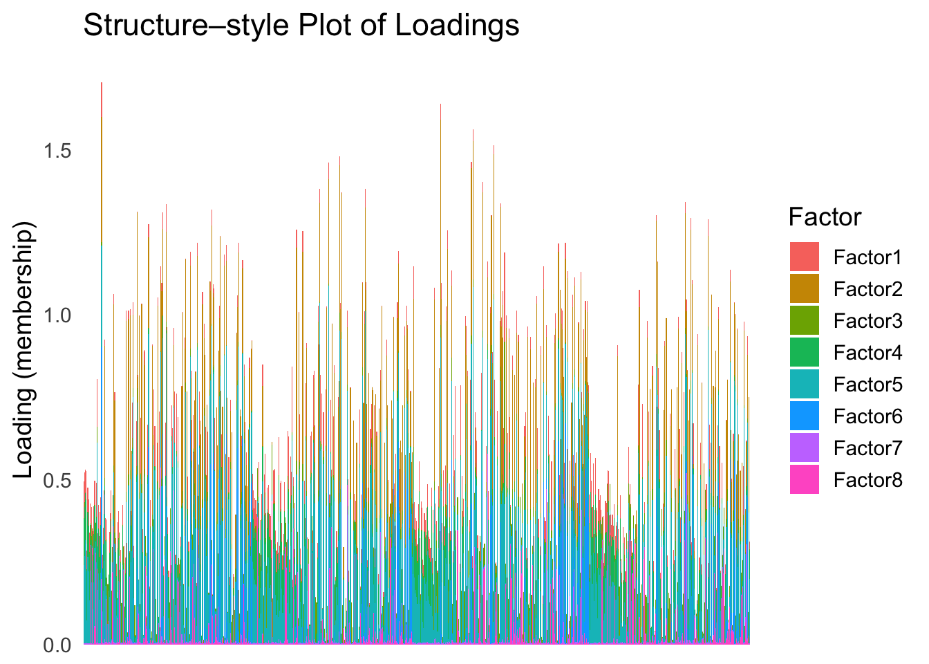

Past versions of unnamed-chunk-3-1.png

Version	Author	Date
2f5e139	Ziang Zhang	2025-07-08

First PC

Now, let’s see how does the result look like when we order the structure plot by the first PC.

PC1 <- prcomp(Loadings,center = TRUE, scale. = FALSE)$x[,1]
PC1_order <- order(PC1)
plot_structure(Loadings, order = rownames(Loadings)[PC1_order])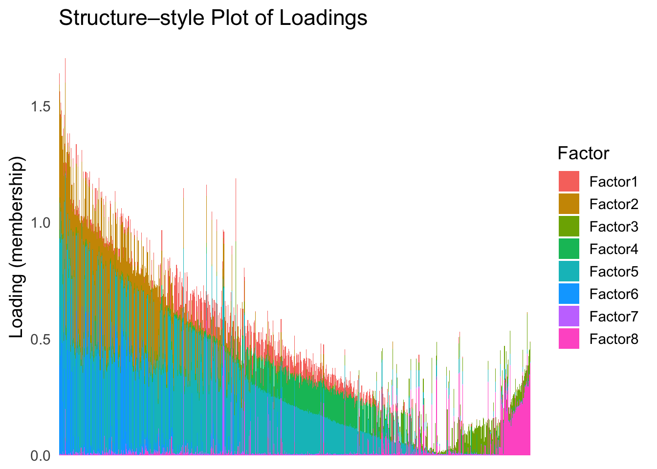

Past versions of unnamed-chunk-4-1.png

Version	Author	Date
2f5e139	Ziang Zhang	2025-07-08

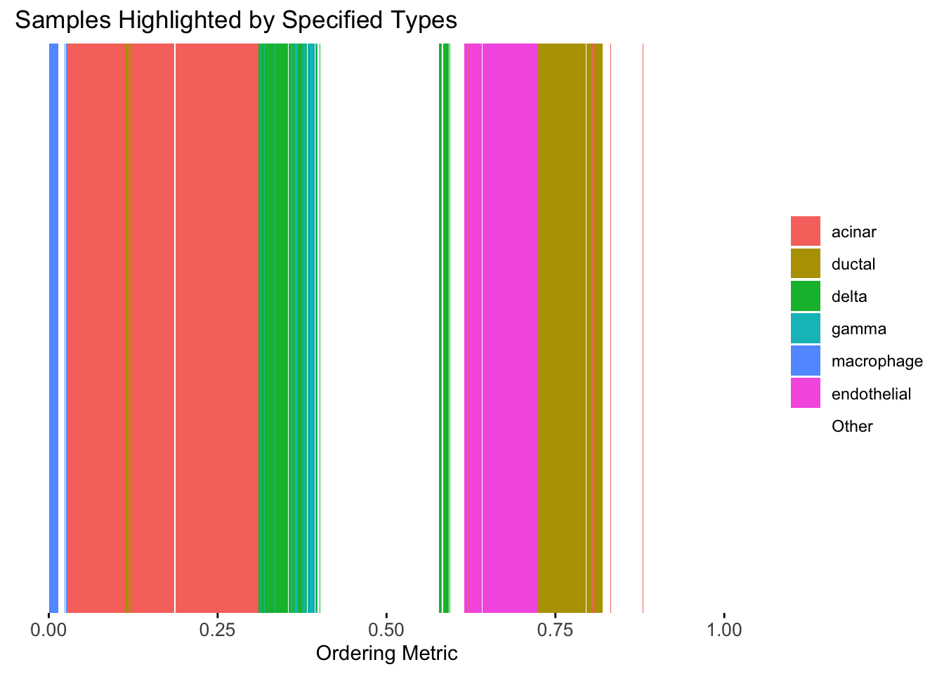
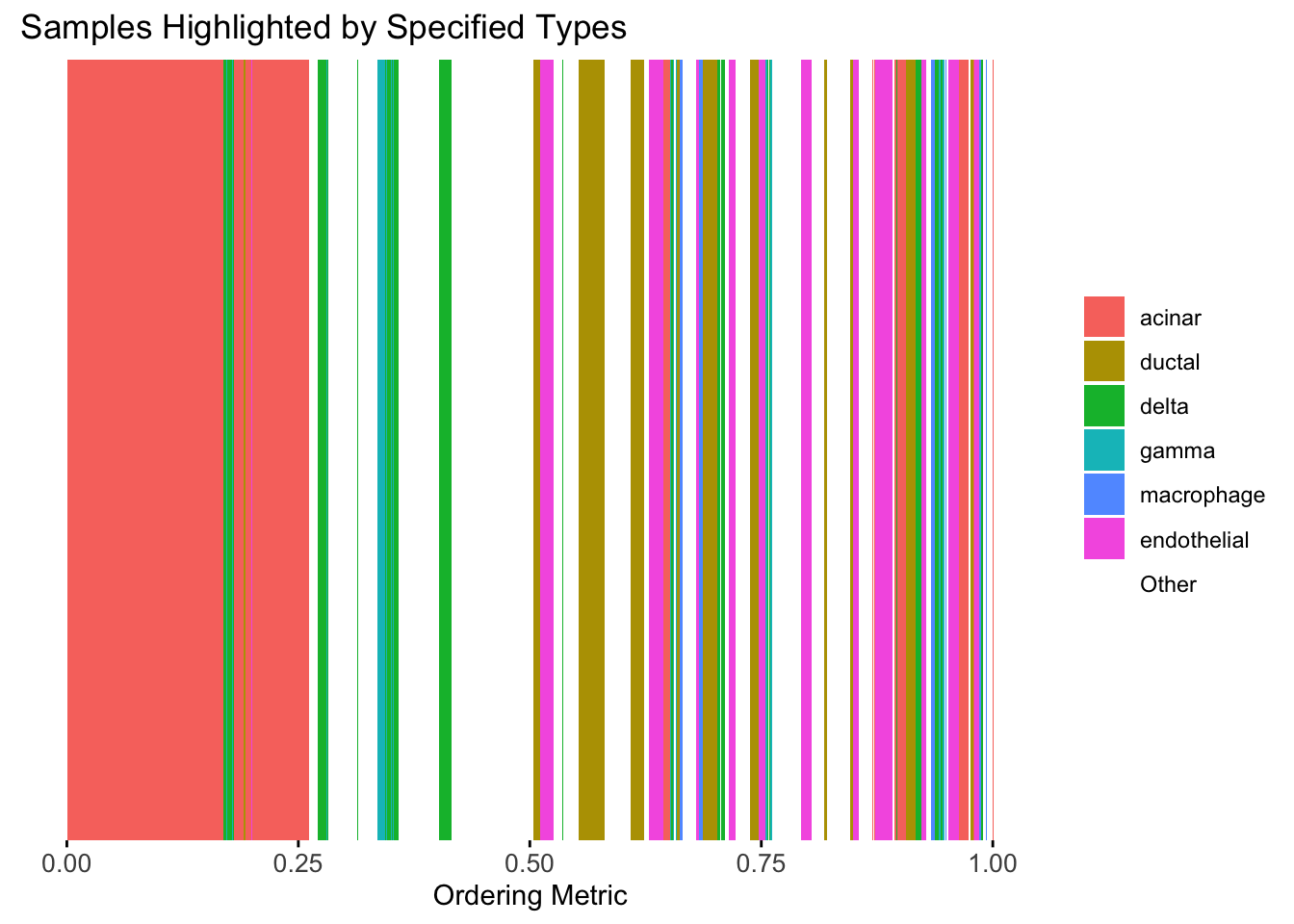
Take a look at the ordering metric versus the cell types.

highlights <- c("acinar","ductal","delta","gamma", "macrophage", "endothelial")
PC1 <- prcomp(Loadings,center = TRUE, scale. = FALSE)$x[,1]
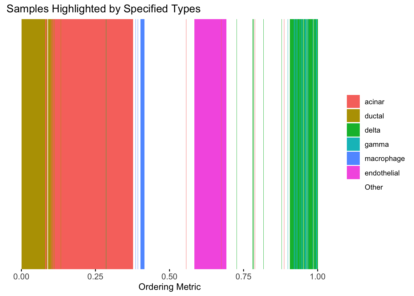
plot_highlight_types(type_vec = celltype,
                     subset_types = highlights,
                     ordering_metric = PC1,
                     other_color = "white"
                     )

Warning: `position_stack()` requires non-overlapping x intervals.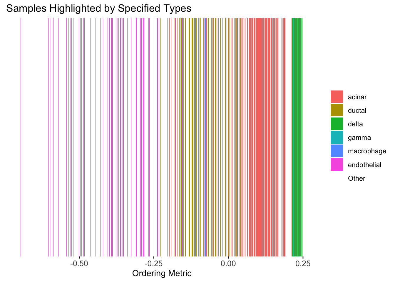

Past versions of unnamed-chunk-5-1.png

Version	Author	Date
2f5e139	Ziang Zhang	2025-07-08

Here the x-axis represents the latent ordering of each cell, and the color represents its cell type. Based on this figure, it appears the first PC distinguishes between (delta, gamma) and (acinar, ductal). However, the ordering could not tell the difference between delta and gamma. Also, the ordering could not distinguish the macrophage from other cell types.

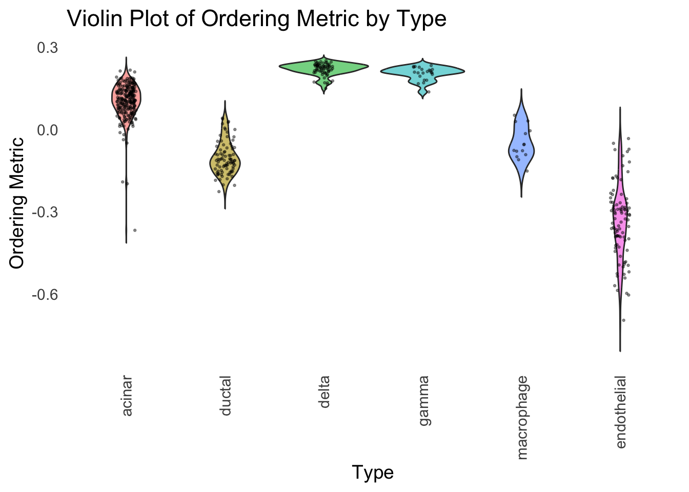
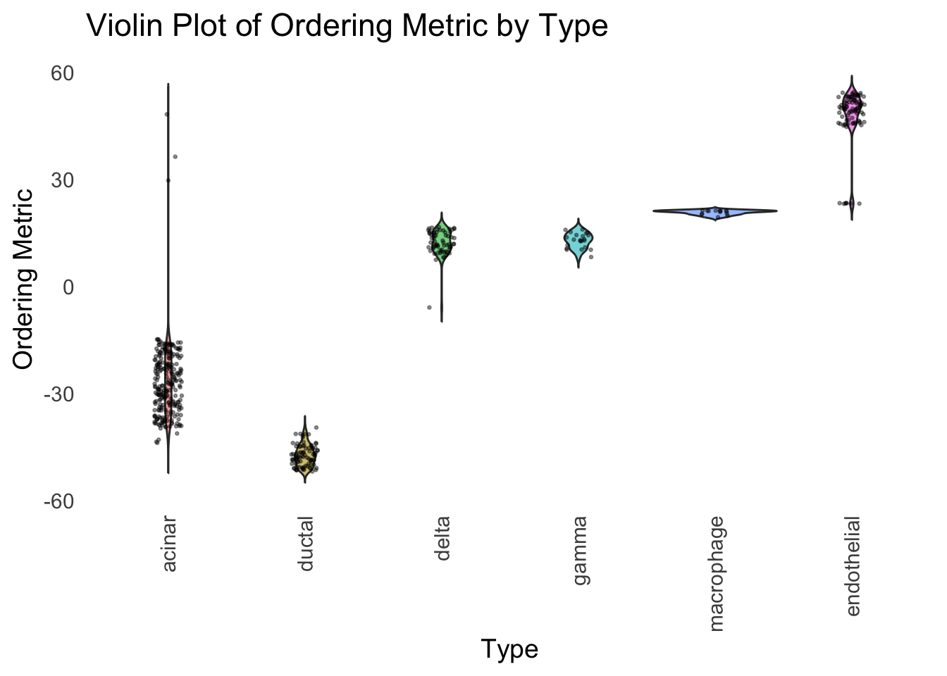
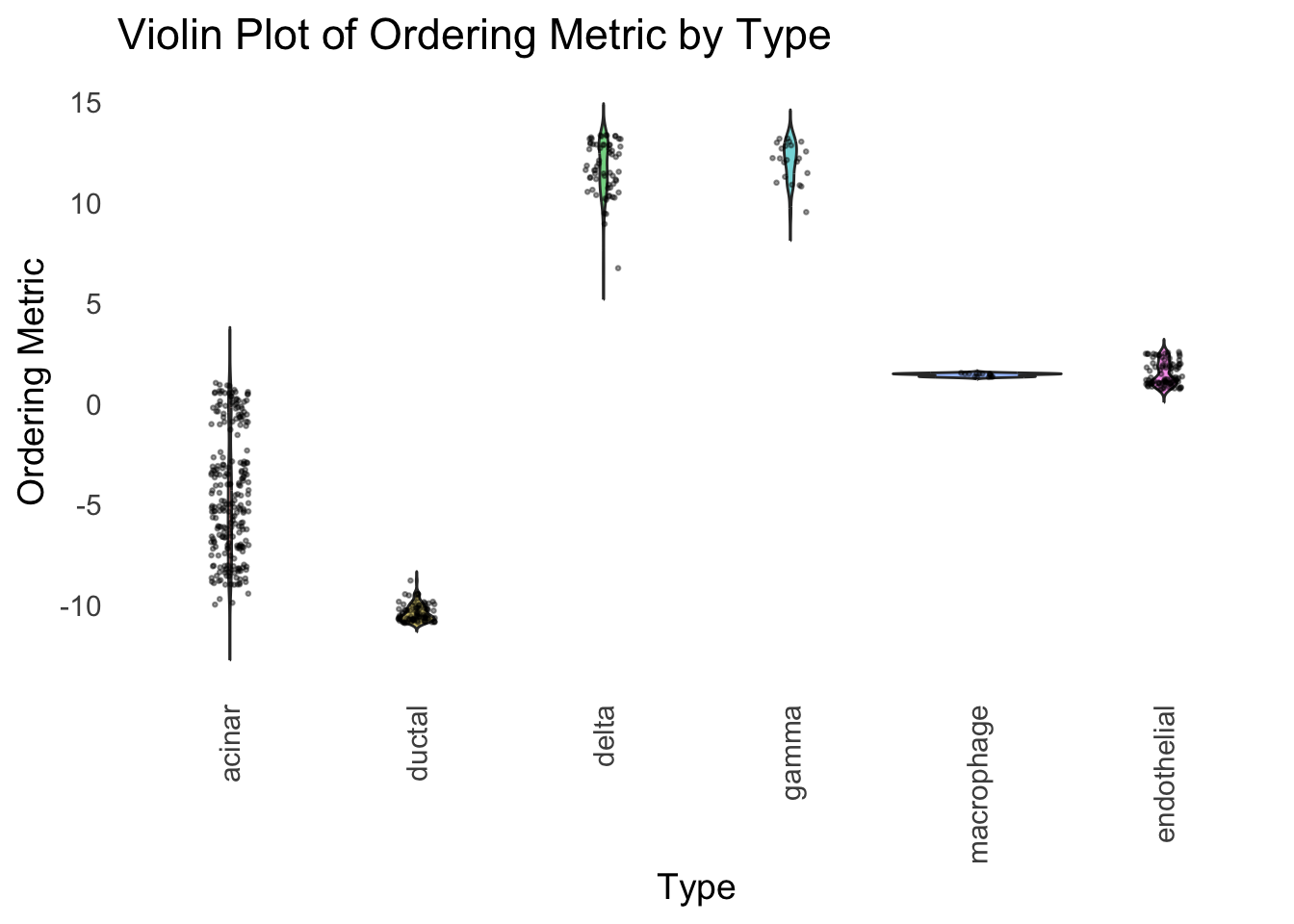
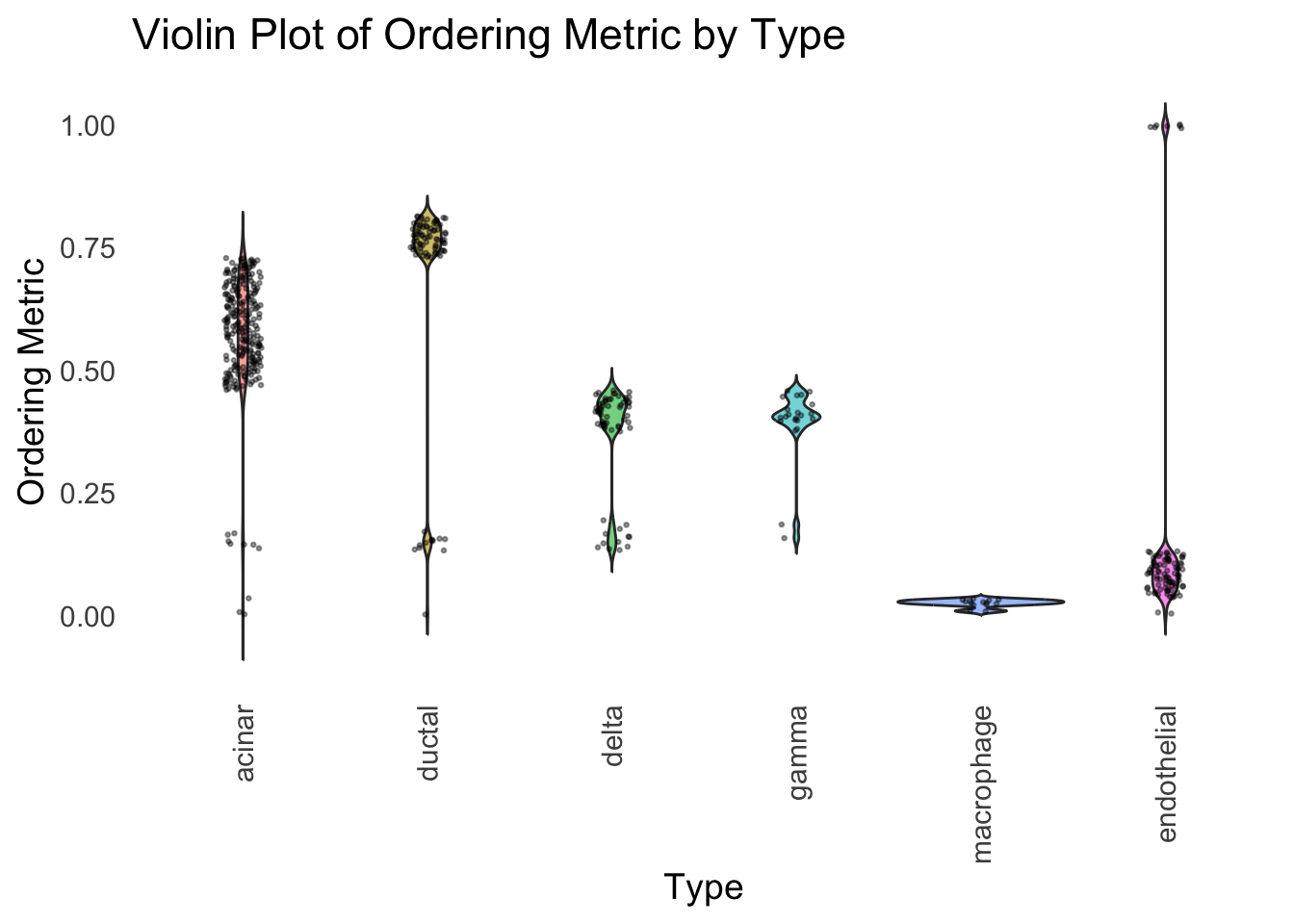
We could also take a look at the distribution of the latent ordering metric for each cell type.

distribution_highlight_types(
  type_vec        = celltype,
  subset_types    = highlights,
  ordering_metric = PC1,
  density         = FALSE
)

Past versions of unnamed-chunk-6-1.png

Version	Author	Date
2f5e139	Ziang Zhang	2025-07-08

The ordering just based on the first PC seems to be not bad. Further since the PC has a probabilistic interpretation, the ordering can also be interpreted probabilistically.

tSNE

Just as a comparison, let’s see how does the result look like when we order the structure plot by the first tSNE.

set.seed(1)
tsne <- Rtsne(Loadings, dims = 1, perplexity = 30, verbose = TRUE, check_duplicates = FALSE)

Performing PCA
Read the 865 x 8 data matrix successfully!
Using no_dims = 1, perplexity = 30.000000, and theta = 0.500000
Computing input similarities...
Building tree...
Done in 0.03 seconds (sparsity = 0.125422)!
Learning embedding...
Iteration 50: error is 61.378493 (50 iterations in 0.03 seconds)
Iteration 100: error is 53.621893 (50 iterations in 0.03 seconds)
Iteration 150: error is 51.570417 (50 iterations in 0.03 seconds)
Iteration 200: error is 50.534836 (50 iterations in 0.03 seconds)
Iteration 250: error is 49.880683 (50 iterations in 0.03 seconds)
Iteration 300: error is 0.892290 (50 iterations in 0.03 seconds)
Iteration 350: error is 0.620483 (50 iterations in 0.03 seconds)
Iteration 400: error is 0.536455 (50 iterations in 0.03 seconds)
Iteration 450: error is 0.508706 (50 iterations in 0.03 seconds)
Iteration 500: error is 0.487135 (50 iterations in 0.03 seconds)
Iteration 550: error is 0.475625 (50 iterations in 0.03 seconds)
Iteration 600: error is 0.463845 (50 iterations in 0.03 seconds)
Iteration 650: error is 0.453710 (50 iterations in 0.03 seconds)
Iteration 700: error is 0.446554 (50 iterations in 0.03 seconds)
Iteration 750: error is 0.439321 (50 iterations in 0.03 seconds)
Iteration 800: error is 0.434766 (50 iterations in 0.03 seconds)
Iteration 850: error is 0.428145 (50 iterations in 0.03 seconds)
Iteration 900: error is 0.424017 (50 iterations in 0.03 seconds)
Iteration 950: error is 0.420721 (50 iterations in 0.03 seconds)
Iteration 1000: error is 0.417580 (50 iterations in 0.03 seconds)
Fitting performed in 0.59 seconds.

tsne_metric <- tsne$Y[,1]
tsne_order <- order(tsne_metric)
names(tsne_metric) <- rownames(Loadings)

plot_structure(Loadings, order = rownames(Loadings)[tsne_order])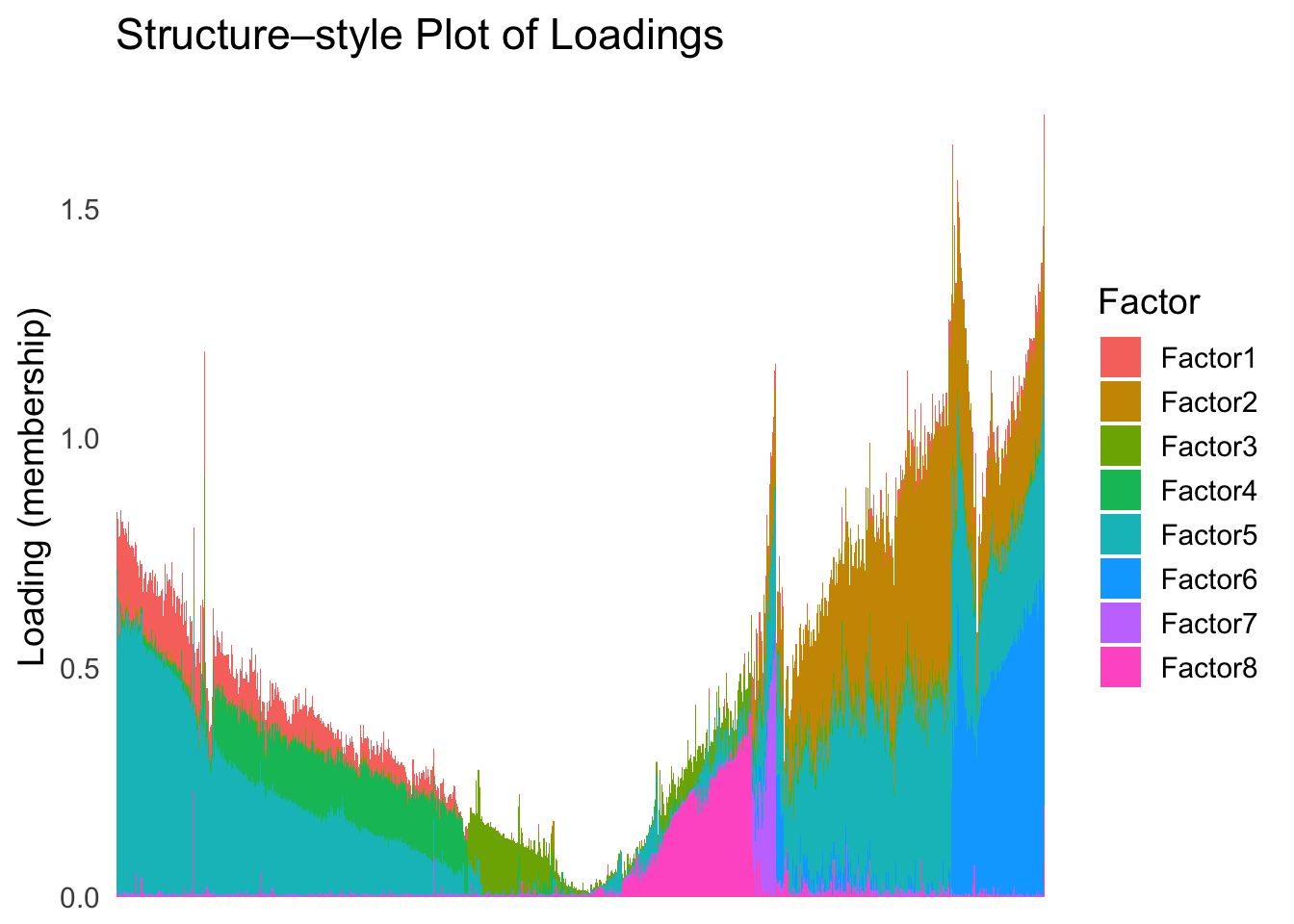

Past versions of unnamed-chunk-8-1.png

Version	Author	Date
2f5e139	Ziang Zhang	2025-07-08

Just based on the structure plot, it seems like the ordering is producing more structured results than the first PC.

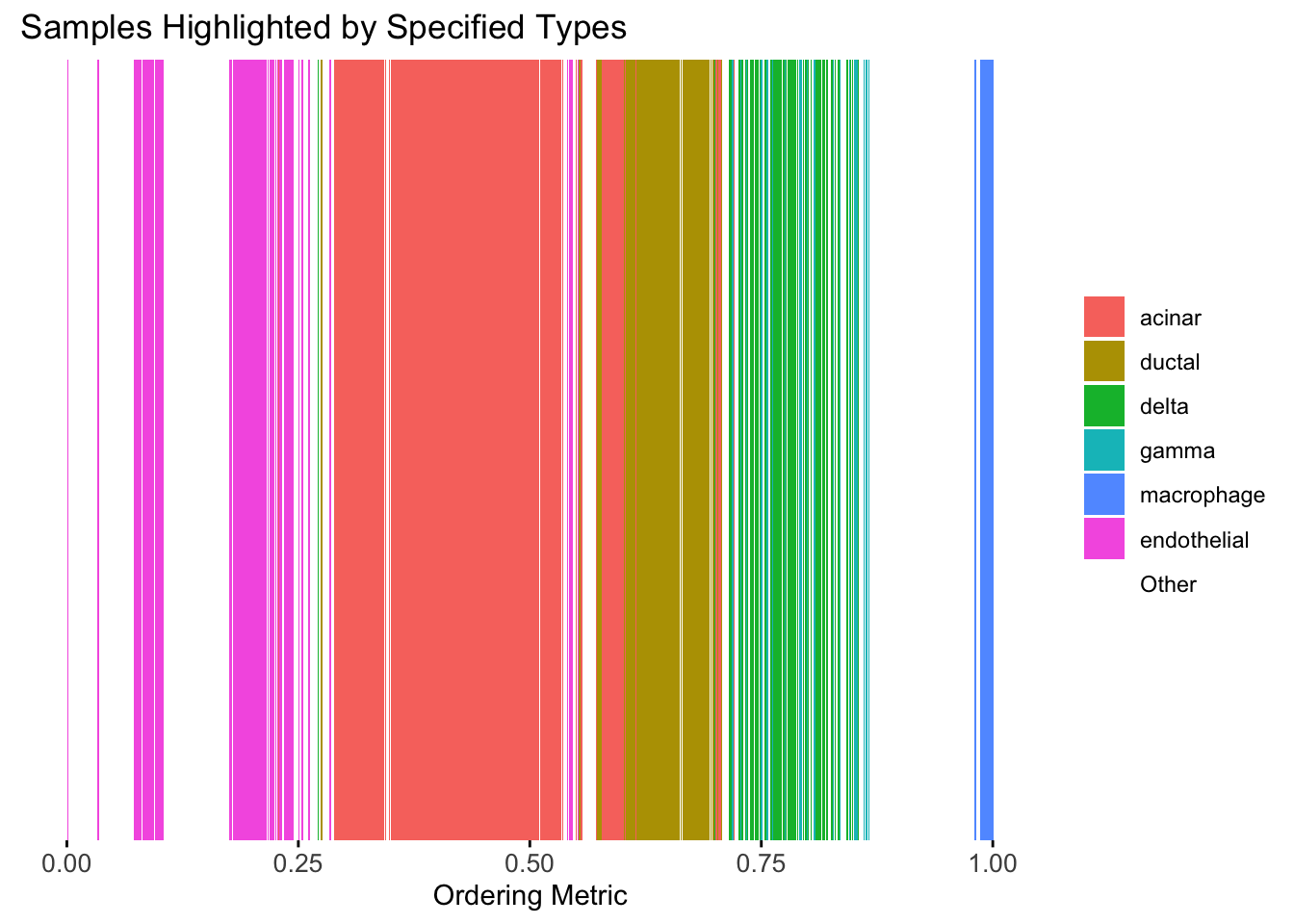
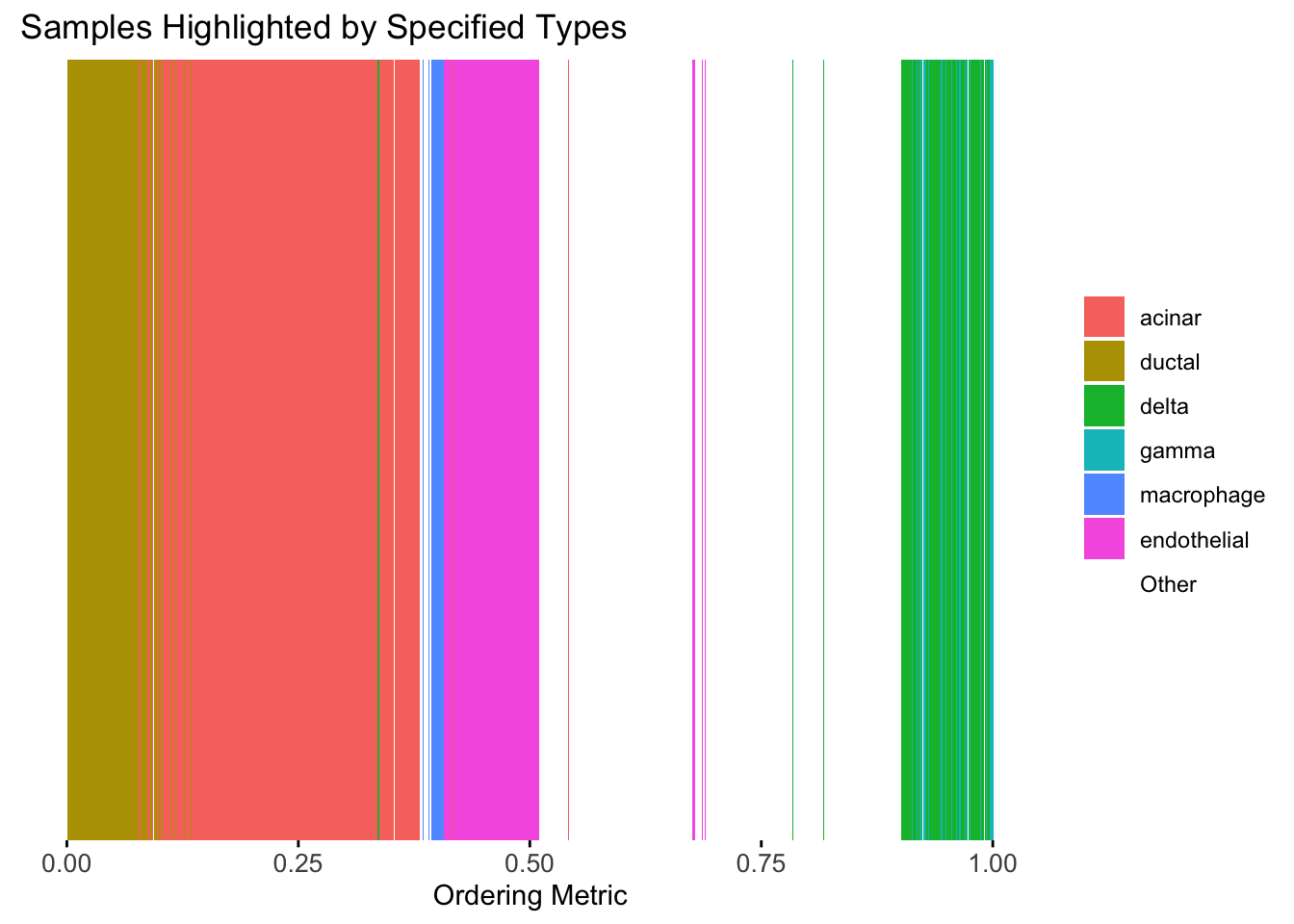
plot_highlight_types(type_vec = celltype,
                     subset_types = highlights,
                     ordering_metric = tsne_metric,
                     other_color = "white"
                     )

Warning: `position_stack()` requires non-overlapping x intervals.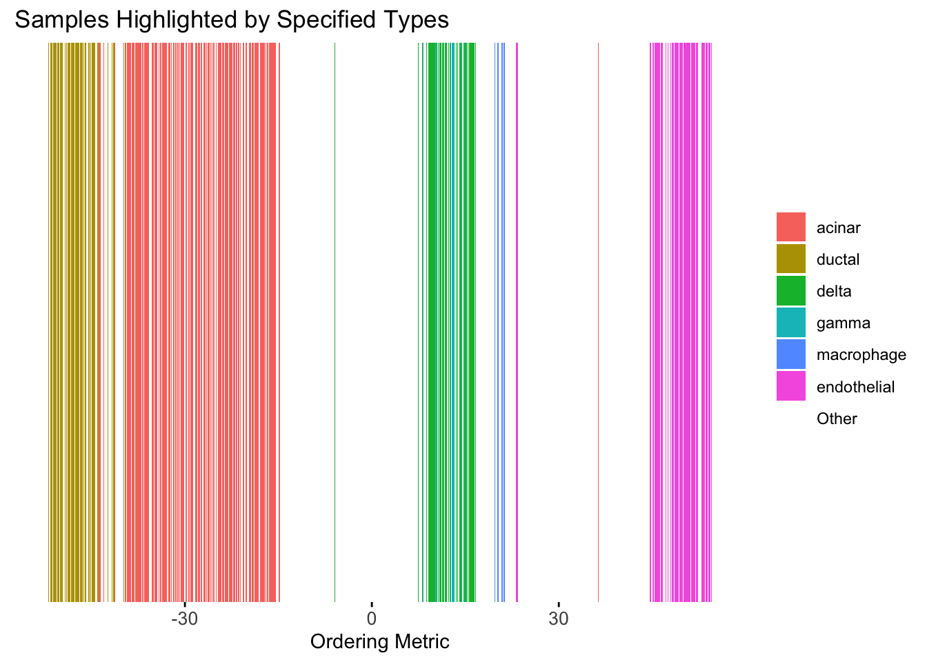

Past versions of unnamed-chunk-9-1.png

Version	Author	Date
2f5e139	Ziang Zhang	2025-07-08

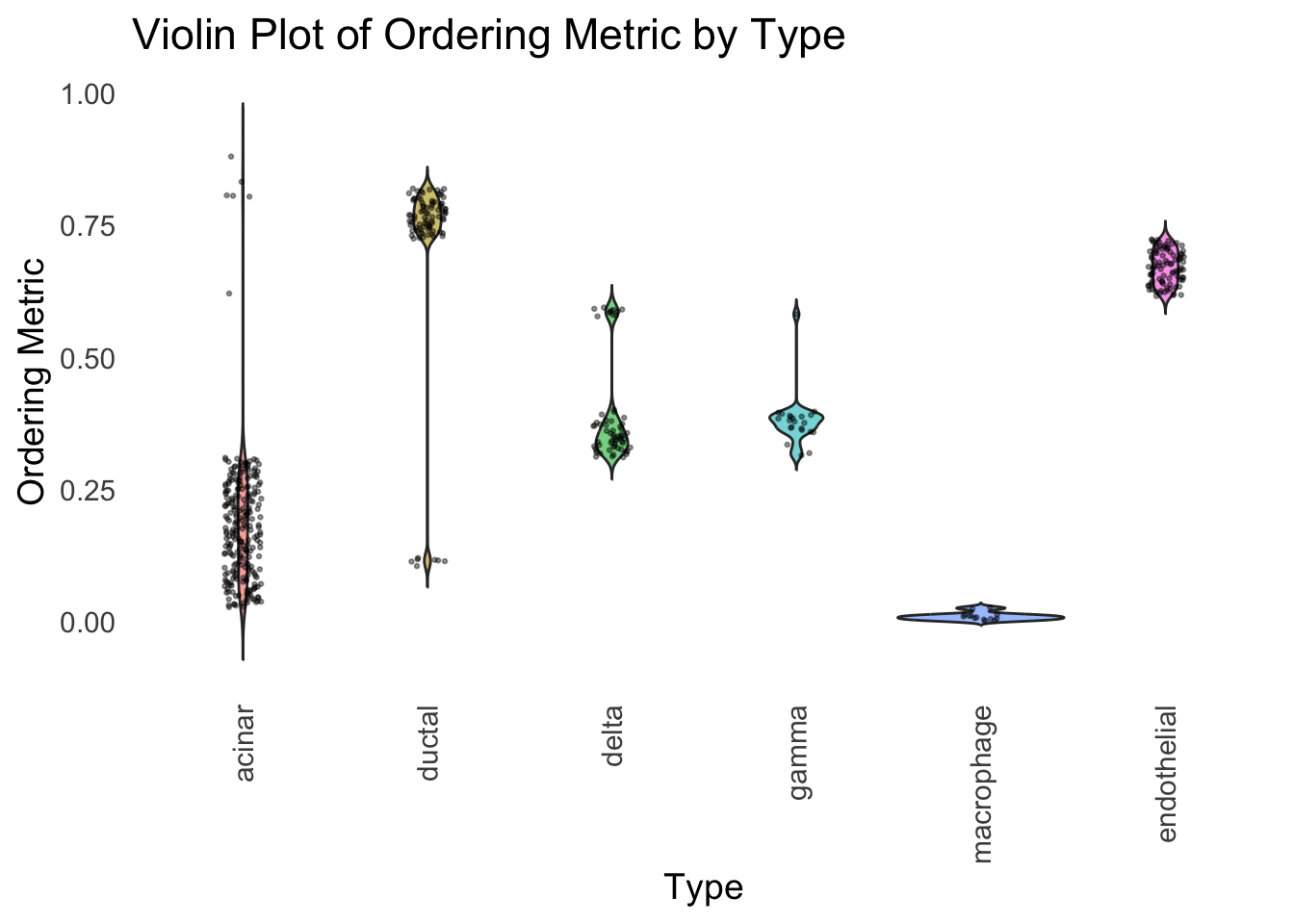
distribution_highlight_types(
  type_vec        = celltype,
  subset_types    = highlights,
  ordering_metric = tsne_metric,
  density         = FALSE
)

Past versions of unnamed-chunk-10-1.png

Version	Author	Date
2f5e139	Ziang Zhang	2025-07-08

Although the tSNE ordering does not have a clear probabilistic interpretation, the structure produced by this ordering matches the cell types much better than the first PC ordering. The distribution of the ordering metric also shows a clear compact separation between the cell types, which is not the case for the first PC. In particular, the macrophage and endothelial cells are now clearly separated from the other cell types.

However, tSNE’s metric only preserves the local structure of the data, and there is no guarantee that the global distance between the points is preserved in the tSNE metric (e.g. the distance between two groups).

UMAP

Let’s see how does the result look like when we order the structure plot by the first UMAP.

umap_result <- umap(Loadings, n_neighbors = 15, min_dist = 0.1, metric = "euclidean")
umap_metric <- umap_result$layout[,1]
names(umap_metric) <- rownames(Loadings)
umap_order <- order(umap_metric)

plot_structure(Loadings, order = rownames(Loadings)[umap_order])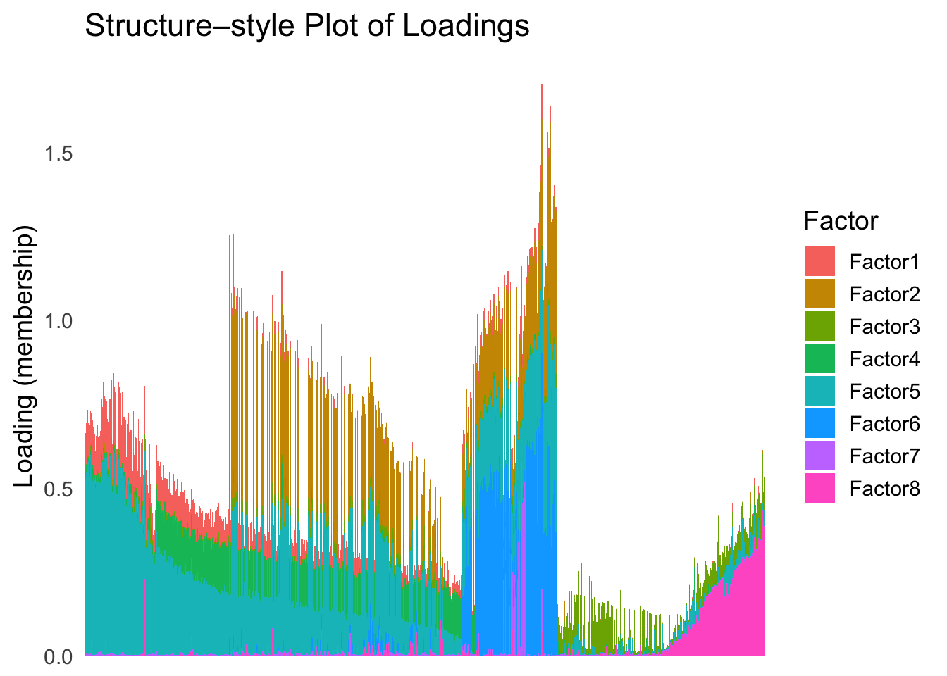

Past versions of unnamed-chunk-12-1.png

Version	Author	Date
2f5e139	Ziang Zhang	2025-07-08

plot_highlight_types(type_vec = celltype,
                     subset_types = highlights,
                     ordering_metric = umap_metric,
                     other_color = "white"
                     )

Warning: `position_stack()` requires non-overlapping x intervals.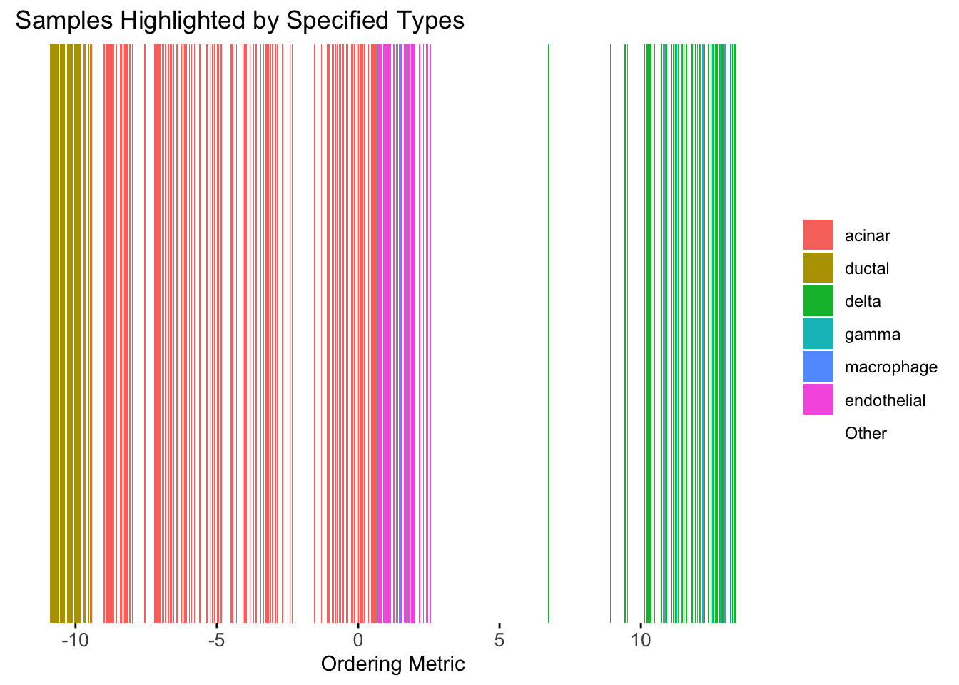

Past versions of unnamed-chunk-13-1.png

Version	Author	Date
2f5e139	Ziang Zhang	2025-07-08

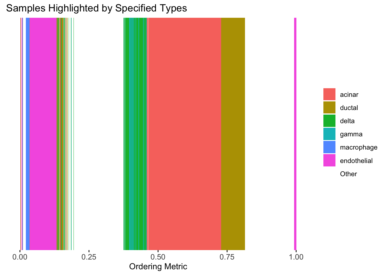
distribution_highlight_types(
  type_vec        = celltype,
  subset_types    = highlights,
  ordering_metric = umap_metric,
  density         = FALSE
)

Past versions of unnamed-chunk-14-1.png

Version	Author	Date
2f5e139	Ziang Zhang	2025-07-08

UMAP can also provide very clear separation between the cell types. However, just like tSNE, it does not have a clear probabilistic interpretation. Furthermore, the global ordering structure from UMAP seems to conflict with the global ordering structure from the tSNE. In the tSNE ordering, acinar is next to delta, which is next to endothelial, where as in the UMAP ordering, acinar is next to endothelial, which is next to delta.

The separation of macrophage is not as clear as in the tSNE ordering.

Hierarchical Clustering

Next, let’s try doing hierarchical clustering on the loadings and see how does the result look like when we order the structure plot by the hierarchical clustering.

First, let’s try when method = single.

hc <- hclust(dist(Loadings), method = "single")
hc_order <- hc$order
names(hc_order) <- rownames(Loadings)

plot_structure(Loadings, order = rownames(Loadings)[hc_order])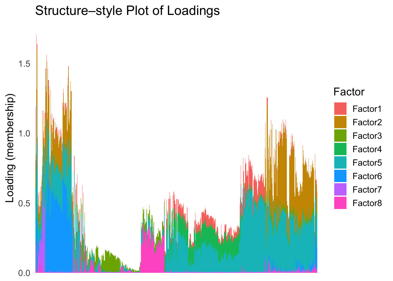

Past versions of unnamed-chunk-16-1.png

Version	Author	Date
2f5e139	Ziang Zhang	2025-07-08

plot_highlight_types(type_vec = celltype,
                     subset_types = highlights,
                     order_vec = rownames(Loadings)[hc_order],
                     other_color = "white"
                     )

Past versions of unnamed-chunk-17-1.png

Version	Author	Date
2f5e139	Ziang Zhang	2025-07-08

distribution_highlight_types(
  type_vec        = celltype,
  subset_types    = highlights,
  order_vec = rownames(Loadings)[hc_order],
  density         = FALSE
)

Past versions of unnamed-chunk-18-1.png

Version	Author	Date
2f5e139	Ziang Zhang	2025-07-08

Similar to t-SNE, the hierarchical clustering ordering also produces a clear separation between the cell types.

Then, let’s try when method = ward.D2.

hc <- hclust(dist(Loadings), method = "ward.D2")
hc_order <- hc$order
names(hc_order) <- rownames(Loadings)

plot_structure(Loadings, order = rownames(Loadings)[hc_order])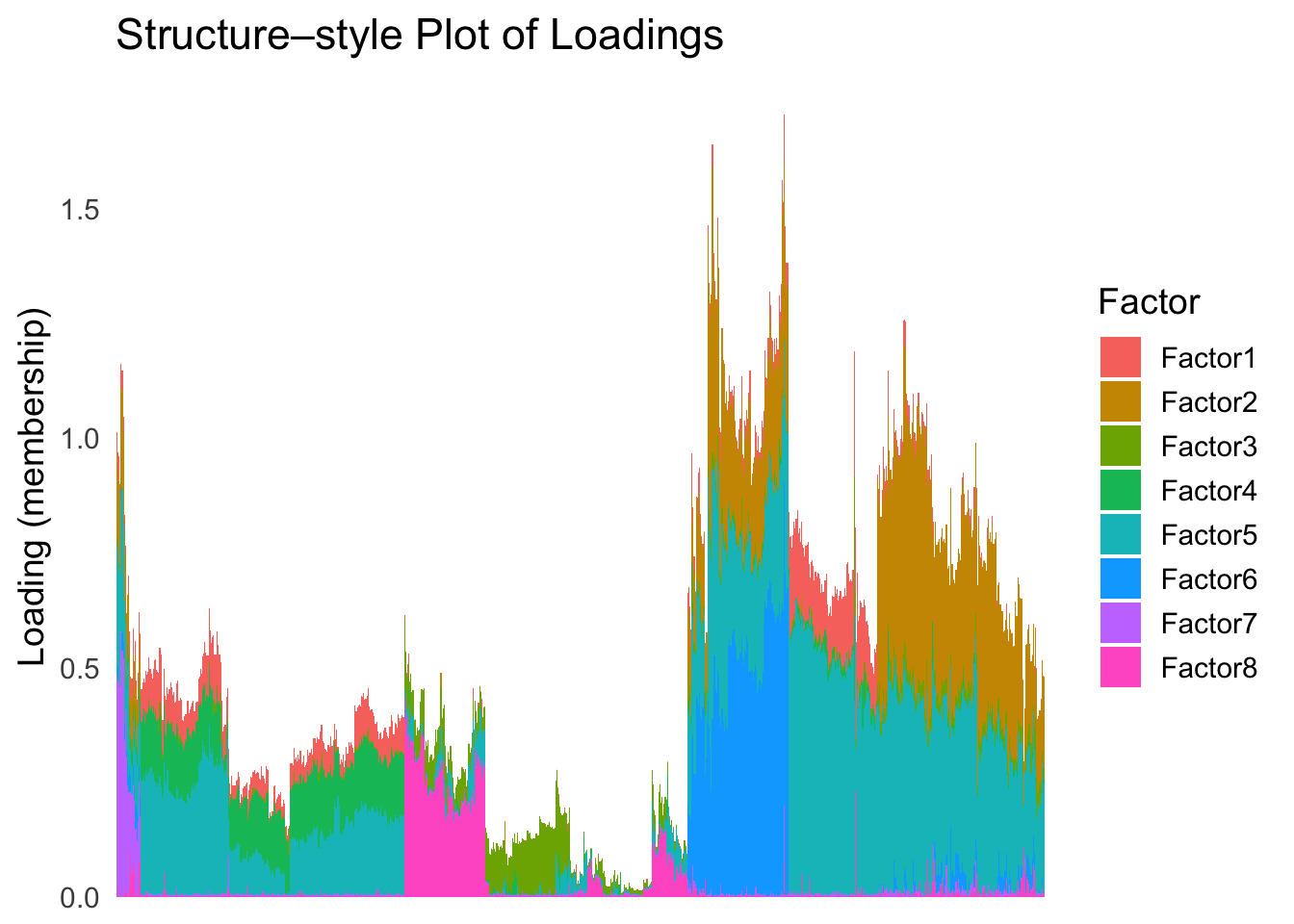

Past versions of unnamed-chunk-20-1.png

Version	Author	Date
2f5e139	Ziang Zhang	2025-07-08

plot_highlight_types(type_vec = celltype,
                     subset_types = highlights,
                     order_vec = rownames(Loadings)[hc_order],
                     other_color = "white"
                     )

Past versions of unnamed-chunk-21-1.png

Version	Author	Date
2f5e139	Ziang Zhang	2025-07-08

distribution_highlight_types(
  type_vec        = celltype,
  subset_types    = highlights,
  order_vec = rownames(Loadings)[hc_order],
  density         = FALSE
)

Past versions of unnamed-chunk-22-1.png

Version	Author	Date
2f5e139	Ziang Zhang	2025-07-08

Again, the hierarchical clustering ordering produces a clear separation between the cell types.

However, just like tSNE and UMAP, the hierarchical clustering ordering does not necessarily produce a interpretable global ordering structure. In particular, the ordering is not unique, as clades of the tree can be rearranged without changing the clustering result.

Ordering based on EM

Now, let’s try to obtain the ordering based on the smooth-EM algorithm.

Traditional EM

First, we will see how the traditional EM algorithm performs on the loadings.

library(mclust)

Package 'mclust' version 6.1.1
Type 'citation("mclust")' for citing this R package in publications.

fit_mclust <- Mclust(Loadings, G=100)

Let’s assume observations in the same cluster are ordered next to each other.

loadings_order_EM <- order(fit_mclust$classification)

plot_structure(Loadings, order = rownames(Loadings)[loadings_order_EM])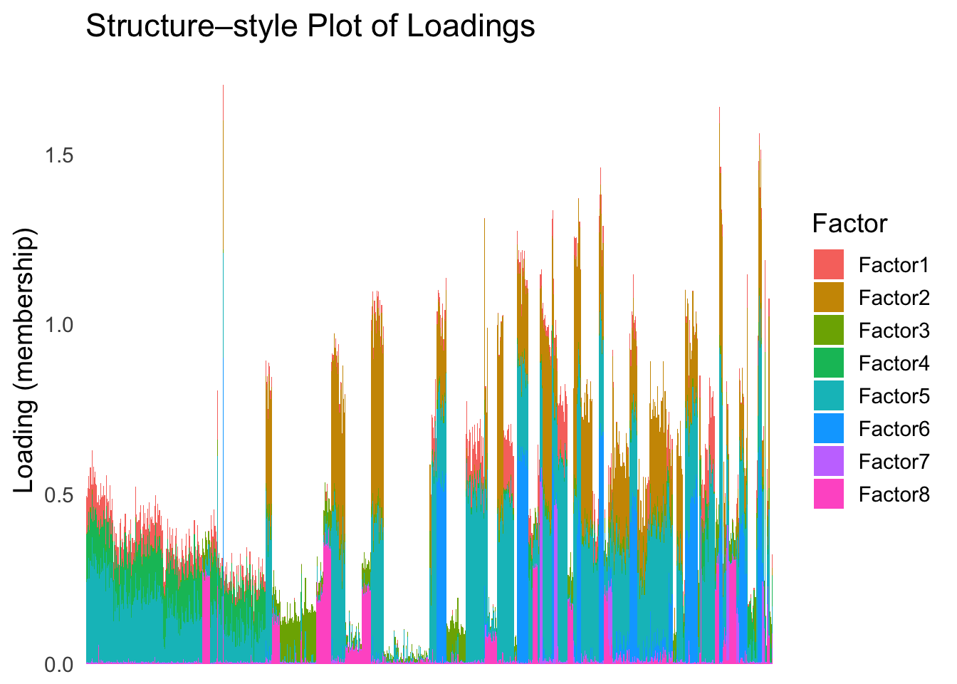

plot_highlight_types(type_vec = celltype,
                     subset_types = highlights,
                     order_vec = rownames(Loadings)[loadings_order_EM],
                     other_color = "white"
                     )

The same cell types tend to be clustered together, but the ordering does not make much sense. This is okay as we know in traditional EM, the index of the cluster is arbitrary.

Smooth-EM with linear prior

source("./code/linear_EM.R")
source("./code/general_EM.R")

Warning: package 'matrixStats' was built under R version 4.3.3

Warning: package 'mvtnorm' was built under R version 4.3.3

Attaching package: 'mvtnorm'

The following object is masked from 'package:mclust':

    dmvnorm

Attaching package: 'Matrix'

The following objects are masked from 'package:tidyr':

    expand, pack, unpack

source("./code/prior_precision.R")
result_linear <- EM_algorithm_linear(
  data = Loadings,
  K = 300,
  betaprec = 0.001,
  seed = 1,
  max_iter = 100,
  verbose = TRUE
)

Iteration   1: objective = 9000.369633
Iteration   2: objective = 10090.984786
Iteration   3: objective = 11677.123012
Iteration   4: objective = 13122.105668
Iteration   5: objective = 14365.551851
Iteration   6: objective = 15650.656488
Iteration   7: objective = 17084.260074
Iteration   8: objective = 18867.723968
Iteration   9: objective = 20309.852222
Iteration  10: objective = 21734.735885
Iteration  11: objective = 22807.979428
Iteration  12: objective = 23585.435901
Iteration  13: objective = 24257.348997
Iteration  14: objective = 24771.595414
Iteration  15: objective = 25124.436676
Iteration  16: objective = 25359.678547
Iteration  17: objective = 25508.305496
Iteration  18: objective = 25601.761928
Iteration  19: objective = 25650.983591
Iteration  20: objective = 25683.153584
Iteration  21: objective = 25704.632332
Iteration  22: objective = 25727.183836
Iteration  23: objective = 25750.591984
Iteration  24: objective = 25765.573937
Iteration  25: objective = 25776.722237
Iteration  26: objective = 25787.843278
Iteration  27: objective = 25798.021246
Iteration  28: objective = 25808.756013
Iteration  29: objective = 25817.933945
Iteration  30: objective = 25827.923133
Iteration  31: objective = 25832.892733
Iteration  32: objective = 25834.937413
Iteration  33: objective = 25836.583470
Iteration  34: objective = 25837.352388
Iteration  35: objective = 25837.290170
Converged at iteration 35 with objective 25837.290170

result_linear$clustering <- apply(result_linear$gamma, 1, which.max)
loadings_order_linear <- order(result_linear$clustering)
plot_structure(Loadings, order = rownames(Loadings)[loadings_order_linear])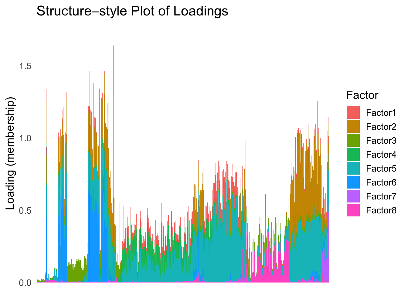

plot_highlight_types(type_vec = celltype,
                     subset_types = highlights,
                     order_vec = rownames(Loadings)[loadings_order_linear],
                     other_color = "white"
                     )

The ordering from linear prior does not look very informative, which is not unexpected since the linear prior is like a coarser version of the PCA.

Smooth-EM with RW1 prior

Now, let’s try the smooth-EM algorithm with a first order random walk prior.

set.seed(1)
Q_prior_RW1 <- make_random_walk_precision(K=100, d=ncol(Loadings), lambda = 100, q=1)
init_params <- make_default_init(Loadings, K=100)
result_RW1 <- EM_algorithm(
  data = Loadings,
  Q_prior = Q_prior_RW1,
  init_params = init_params,
  max_iter = 100,
  modelName = "EII",
  tol = 1e-5,
  verbose = TRUE
)

Iteration 1: objective = 7400.4641
Iteration 2: objective = 7404.8029
Iteration 3: objective = 7446.8542
Iteration 4: objective = 7767.8426
Iteration 5: objective = 8750.8617
Iteration 6: objective = 9647.5658
Iteration 7: objective = 10635.3860
Iteration 8: objective = 11617.9350
Iteration 9: objective = 12398.8647
Iteration 10: objective = 12774.2315
Iteration 11: objective = 12943.7901
Iteration 12: objective = 13043.6552
Iteration 13: objective = 13099.3848
Iteration 14: objective = 13133.0113
Iteration 15: objective = 13159.2779
Iteration 16: objective = 13175.1134
Iteration 17: objective = 13187.5853
Iteration 18: objective = 13210.1739
Iteration 19: objective = 13232.3480
Iteration 20: objective = 13241.6946
Iteration 21: objective = 13247.4560
Iteration 22: objective = 13251.3146
Iteration 23: objective = 13254.0073
Iteration 24: objective = 13255.9540
Iteration 25: objective = 13257.4111
Iteration 26: objective = 13258.5356
Iteration 27: objective = 13259.4256
Iteration 28: objective = 13260.1468
Iteration 29: objective = 13260.7461
Iteration 30: objective = 13261.2588
Iteration 31: objective = 13261.7119
Iteration 32: objective = 13262.1256
Iteration 33: objective = 13262.5140
Iteration 34: objective = 13262.8859
Iteration 35: objective = 13263.2456
Iteration 36: objective = 13263.5936
Iteration 37: objective = 13263.9276
Iteration 38: objective = 13264.2436
Iteration 39: objective = 13264.5371
Iteration 40: objective = 13264.8039
Iteration 41: objective = 13265.0412
Iteration 42: objective = 13265.2473
Iteration 43: objective = 13265.4222
Iteration 44: objective = 13265.5672
Iteration 45: objective = 13265.6847
Iteration 46: objective = 13265.7776
Iteration 47: objective = 13265.8490
Iteration 48: objective = 13265.9022
Iteration 49: objective = 13265.9403
Iteration 50: objective = 13265.9661
Iteration 51: objective = 13265.9821
Iteration 52: objective = 13265.9904
Iteration 53: objective = 13265.9927
Converged at iteration 54 with objective 13265.9905

result_RW1$clustering <- apply(result_RW1$gamma, 1, which.max)
loadings_order_RW1 <- order(result_RW1$clustering)
plot_structure(Loadings, order = rownames(Loadings)[loadings_order_RW1])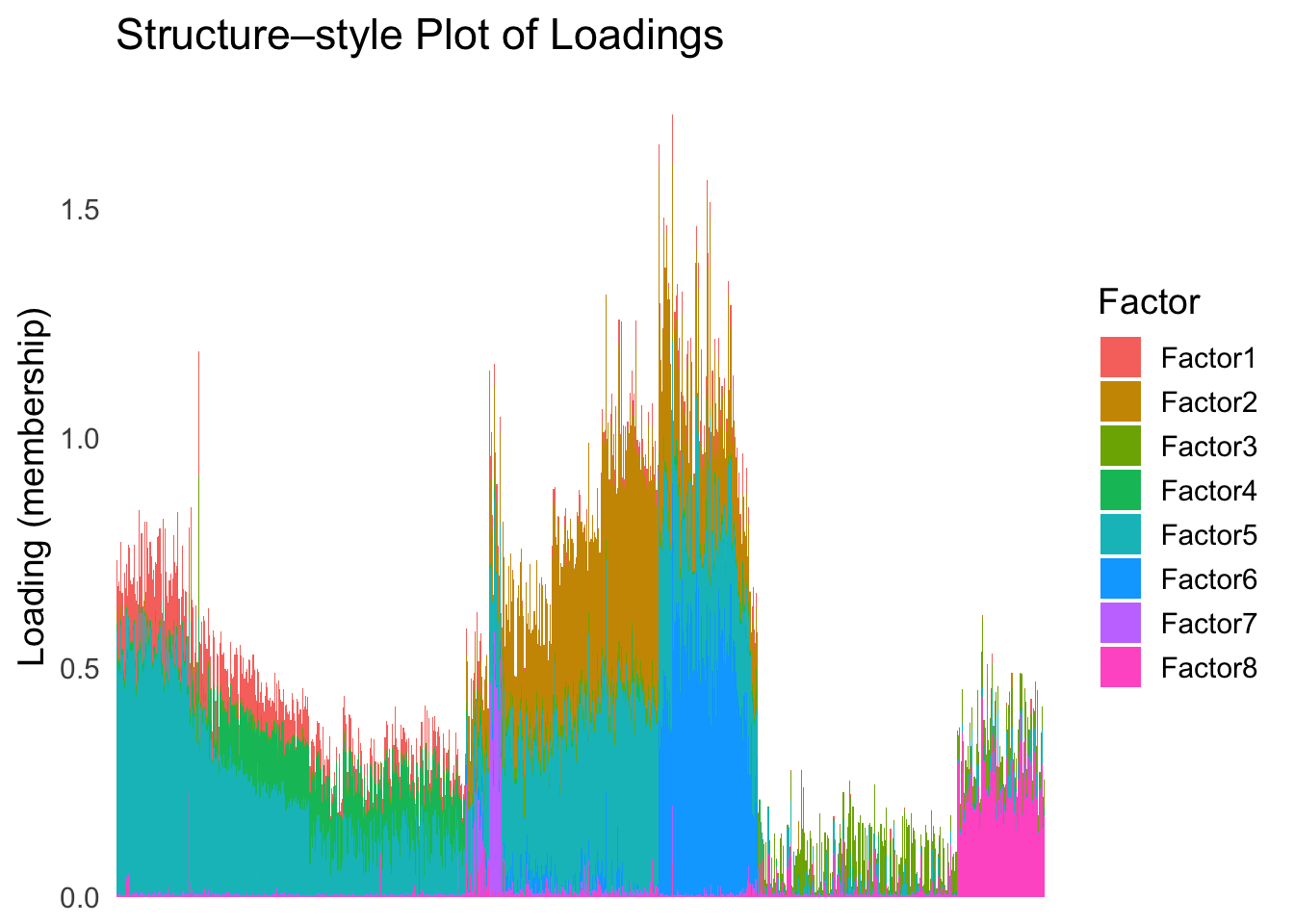

plot_highlight_types(type_vec = celltype,
                     subset_types = highlights,
                     order_vec = rownames(Loadings)[loadings_order_RW1],
                     other_color = "white"
                     )

The result from RW1 looks good. Each cell type is separated from the others, and the ordering seems to make sense.

Smooth-EM with RW2 prior

Next, we will try the RW2 prior in the smooth-EM algorithm.

Q_prior_RW2 <- make_random_walk_precision(K=100, d=ncol(Loadings), lambda = 1000, q=2)
result_RW2 <- EM_algorithm(
  data = Loadings,
  Q_prior = Q_prior_RW2,
  init_params = init_params,
  max_iter = 300,
  modelName = "EII",
  tol = 1e-5,
  verbose = TRUE
)

Iteration 1: objective = 8312.5101
Iteration 2: objective = 8319.7097
Iteration 3: objective = 8400.4678
Iteration 4: objective = 8979.9229
Iteration 5: objective = 10026.7426
Iteration 6: objective = 10918.0549
Iteration 7: objective = 12621.1532
Iteration 8: objective = 13722.5287
Iteration 9: objective = 14240.3743
Iteration 10: objective = 14502.8912
Iteration 11: objective = 14690.2165
Iteration 12: objective = 14811.4430
Iteration 13: objective = 14915.9464
Iteration 14: objective = 15008.8120
Iteration 15: objective = 15087.0693
Iteration 16: objective = 15155.1829
Iteration 17: objective = 15223.5622
Iteration 18: objective = 15295.3476
Iteration 19: objective = 15354.6444
Iteration 20: objective = 15407.8951
Iteration 21: objective = 15457.7666
Iteration 22: objective = 15498.2489
Iteration 23: objective = 15531.2266
Iteration 24: objective = 15556.1943
Iteration 25: objective = 15577.5501
Iteration 26: objective = 15594.5084
Iteration 27: objective = 15608.8738
Iteration 28: objective = 15622.5929
Iteration 29: objective = 15634.1777
Iteration 30: objective = 15642.1329
Iteration 31: objective = 15648.3680
Iteration 32: objective = 15656.1015
Iteration 33: objective = 15666.3914
Iteration 34: objective = 15674.4580
Iteration 35: objective = 15679.5330
Iteration 36: objective = 15684.5742
Iteration 37: objective = 15690.1435
Iteration 38: objective = 15695.9500
Iteration 39: objective = 15703.7122
Iteration 40: objective = 15712.3576
Iteration 41: objective = 15718.6916
Iteration 42: objective = 15722.2593
Iteration 43: objective = 15724.6795
Iteration 44: objective = 15727.5857
Iteration 45: objective = 15730.5362
Iteration 46: objective = 15734.3871
Iteration 47: objective = 15739.8149
Iteration 48: objective = 15745.0370
Iteration 49: objective = 15749.2871
Iteration 50: objective = 15752.4081
Iteration 51: objective = 15754.9334
Iteration 52: objective = 15758.4964
Iteration 53: objective = 15763.4665
Iteration 54: objective = 15767.0124
Iteration 55: objective = 15769.3160
Iteration 56: objective = 15772.4248
Iteration 57: objective = 15777.5482
Iteration 58: objective = 15783.9405
Iteration 59: objective = 15790.3024
Iteration 60: objective = 15795.5554
Iteration 61: objective = 15798.8527
Iteration 62: objective = 15801.0477
Iteration 63: objective = 15803.0848
Iteration 64: objective = 15805.6896
Iteration 65: objective = 15808.9195
Iteration 66: objective = 15811.9902
Iteration 67: objective = 15815.0200
Iteration 68: objective = 15818.5022
Iteration 69: objective = 15822.5847
Iteration 70: objective = 15826.2054
Iteration 71: objective = 15829.0675
Iteration 72: objective = 15831.8108
Iteration 73: objective = 15833.7451
Iteration 74: objective = 15834.9587
Iteration 75: objective = 15836.0208
Iteration 76: objective = 15837.4377
Iteration 77: objective = 15839.5974
Iteration 78: objective = 15842.5106
Iteration 79: objective = 15845.7941
Iteration 80: objective = 15849.0930
Iteration 81: objective = 15852.3393
Iteration 82: objective = 15855.6113
Iteration 83: objective = 15858.9370
Iteration 84: objective = 15861.0288
Iteration 85: objective = 15862.0126
Iteration 86: objective = 15862.9482
Iteration 87: objective = 15863.9877
Iteration 88: objective = 15865.1048
Iteration 89: objective = 15866.4606
Iteration 90: objective = 15868.3884
Iteration 91: objective = 15871.1821
Iteration 92: objective = 15874.7395
Iteration 93: objective = 15878.5338
Iteration 94: objective = 15882.0466
Iteration 95: objective = 15885.0449
Iteration 96: objective = 15887.5562
Iteration 97: objective = 15889.6412
Iteration 98: objective = 15891.0735
Iteration 99: objective = 15891.9653
Iteration 100: objective = 15893.0371
Iteration 101: objective = 15894.7001
Iteration 102: objective = 15896.6561
Iteration 103: objective = 15899.1740
Iteration 104: objective = 15902.4640
Iteration 105: objective = 15906.0594
Iteration 106: objective = 15909.4853
Iteration 107: objective = 15912.5164
Iteration 108: objective = 15915.0794
Iteration 109: objective = 15917.1597
Iteration 110: objective = 15918.7799
Iteration 111: objective = 15920.0033
Iteration 112: objective = 15920.9311
Iteration 113: objective = 15921.7072
Iteration 114: objective = 15922.5167
Iteration 115: objective = 15923.5115
Iteration 116: objective = 15924.7572
Iteration 117: objective = 15926.4261
Iteration 118: objective = 15929.0117
Iteration 119: objective = 15932.9452
Iteration 120: objective = 15937.5178
Iteration 121: objective = 15941.7716
Iteration 122: objective = 15945.3556
Iteration 123: objective = 15948.2022
Iteration 124: objective = 15950.4021
Iteration 125: objective = 15952.1622
Iteration 126: objective = 15953.3570
Iteration 127: objective = 15953.6938
Iteration 128: objective = 15953.7289
Iteration 129: objective = 15953.8868
Iteration 130: objective = 15954.2423
Iteration 131: objective = 15954.8295
Iteration 132: objective = 15955.7711
Iteration 133: objective = 15957.1776
Iteration 134: objective = 15958.8118
Iteration 135: objective = 15960.4928
Iteration 136: objective = 15962.4626
Iteration 137: objective = 15964.8530
Iteration 138: objective = 15967.6641
Iteration 139: objective = 15970.8526
Iteration 140: objective = 15973.9971
Iteration 141: objective = 15976.5595
Iteration 142: objective = 15978.5208
Iteration 143: objective = 15979.9771
Iteration 144: objective = 15981.0058
Iteration 145: objective = 15981.7263
Iteration 146: objective = 15982.2615
Iteration 147: objective = 15982.7077
Iteration 148: objective = 15983.1361
Iteration 149: objective = 15983.6091
Iteration 150: objective = 15984.2051
Iteration 151: objective = 15985.0294
Iteration 152: objective = 15986.1217
Iteration 153: objective = 15987.3295
Iteration 154: objective = 15988.6553
Iteration 155: objective = 15990.2511
Iteration 156: objective = 15992.0018
Iteration 157: objective = 15993.7038
Iteration 158: objective = 15995.2475
Iteration 159: objective = 15996.6159
Iteration 160: objective = 15997.8461
Iteration 161: objective = 15999.0275
Iteration 162: objective = 16000.3326
Iteration 163: objective = 16001.9482
Iteration 164: objective = 16003.7755
Iteration 165: objective = 16005.6044
Iteration 166: objective = 16007.5233
Iteration 167: objective = 16009.2591
Iteration 168: objective = 16010.4835
Iteration 169: objective = 16011.2715
Iteration 170: objective = 16011.8007
Iteration 171: objective = 16012.2078
Iteration 172: objective = 16012.6239
Iteration 173: objective = 16013.1949
Iteration 174: objective = 16013.8843
Iteration 175: objective = 16014.4308
Iteration 176: objective = 16014.9800
Iteration 177: objective = 16015.9720
Iteration 178: objective = 16017.6391
Iteration 179: objective = 16019.8875
Iteration 180: objective = 16022.3939
Iteration 181: objective = 16024.8444
Iteration 182: objective = 16027.0760
Iteration 183: objective = 16029.0477
Iteration 184: objective = 16030.7630
Iteration 185: objective = 16032.2189
Iteration 186: objective = 16033.3705
Iteration 187: objective = 16034.1276
Iteration 188: objective = 16034.5729
Iteration 189: objective = 16034.9604
Iteration 190: objective = 16035.2527
Iteration 191: objective = 16035.3855
Iteration 192: objective = 16035.5456
Iteration 193: objective = 16035.8929
Iteration 194: objective = 16036.5151
Iteration 195: objective = 16037.5181
Iteration 196: objective = 16039.0074
Iteration 197: objective = 16040.9897
Iteration 198: objective = 16043.3184
Iteration 199: objective = 16045.7750
Iteration 200: objective = 16048.2060
Iteration 201: objective = 16050.6007
Iteration 202: objective = 16053.0211
Iteration 203: objective = 16055.2855
Iteration 204: objective = 16057.1498
Iteration 205: objective = 16058.6444
Iteration 206: objective = 16059.8624
Iteration 207: objective = 16060.8600
Iteration 208: objective = 16061.6709
Iteration 209: objective = 16062.3241
Iteration 210: objective = 16062.8491
Iteration 211: objective = 16063.2734
Iteration 212: objective = 16063.6198
Iteration 213: objective = 16063.9044
Iteration 214: objective = 16064.1370
Iteration 215: objective = 16064.3238
Iteration 216: objective = 16064.4732
Iteration 217: objective = 16064.6056
Iteration 218: objective = 16064.7583
Iteration 219: objective = 16064.9691
Iteration 220: objective = 16065.2505
Iteration 221: objective = 16065.6284
Iteration 222: objective = 16066.1647
Iteration 223: objective = 16066.8341
Iteration 224: objective = 16067.3458
Iteration 225: objective = 16067.7147
Iteration 226: objective = 16068.4277
Iteration 227: objective = 16069.6652
Iteration 228: objective = 16071.4987
Iteration 229: objective = 16073.9146
Iteration 230: objective = 16076.6455
Iteration 231: objective = 16079.3293
Iteration 232: objective = 16081.7391
Iteration 233: objective = 16083.8077
Iteration 234: objective = 16085.5509
Iteration 235: objective = 16087.0114
Iteration 236: objective = 16088.2369
Iteration 237: objective = 16089.2741
Iteration 238: objective = 16090.1663
Iteration 239: objective = 16090.9492
Iteration 240: objective = 16091.6484
Iteration 241: objective = 16092.2828
Iteration 242: objective = 16092.8728
Iteration 243: objective = 16093.4451
Iteration 244: objective = 16094.0338
Iteration 245: objective = 16094.6796
Iteration 246: objective = 16095.4291
Iteration 247: objective = 16096.3333
Iteration 248: objective = 16097.4396
Iteration 249: objective = 16098.7757
Iteration 250: objective = 16100.3285
Iteration 251: objective = 16102.0305
Iteration 252: objective = 16103.7747
Iteration 253: objective = 16105.4526
Iteration 254: objective = 16106.9868
Iteration 255: objective = 16108.3376
Iteration 256: objective = 16109.4956
Iteration 257: objective = 16110.4753
Iteration 258: objective = 16111.3152
Iteration 259: objective = 16112.0883
Iteration 260: objective = 16112.9050
Iteration 261: objective = 16113.8335
Iteration 262: objective = 16114.7107
Iteration 263: objective = 16115.2945
Iteration 264: objective = 16115.6691
Iteration 265: objective = 16116.0095
Iteration 266: objective = 16116.3628
Iteration 267: objective = 16116.7300
Iteration 268: objective = 16117.1125
Iteration 269: objective = 16117.5102
Iteration 270: objective = 16117.9212
Iteration 271: objective = 16118.3527
Iteration 272: objective = 16118.8139
Iteration 273: objective = 16119.1688
Converged at iteration 274 with objective 16119.1339

result_RW2$clustering <- apply(result_RW2$gamma, 1, which.max)
loadings_order_RW2 <- order(result_RW2$clustering)
plot_structure(Loadings, order = rownames(Loadings)[loadings_order_RW2])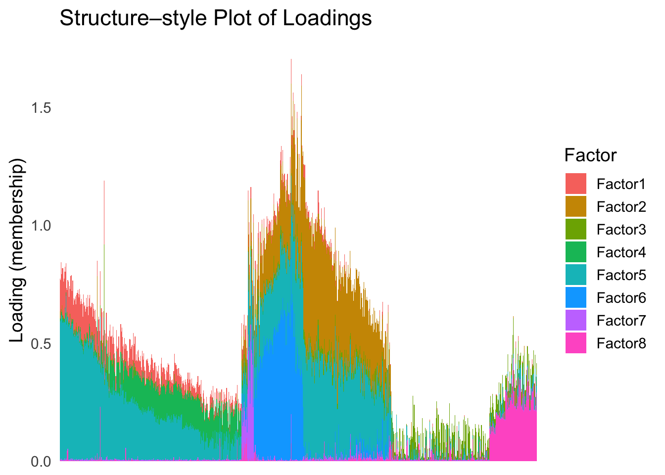

plot_highlight_types(type_vec = celltype,
                     subset_types = highlights,
                     order_vec = rownames(Loadings)[loadings_order_RW2],
                     other_color = "white"
                     )

The result also looks good, but the choice of the smoothing parameter (lambda) is very important…

Session information

sessionInfo()

R version 4.3.1 (2023-06-16)
Platform: aarch64-apple-darwin20 (64-bit)
Running under: macOS Monterey 12.7.4

Matrix products: default
BLAS:   /Library/Frameworks/R.framework/Versions/4.3-arm64/Resources/lib/libRblas.0.dylib 
LAPACK: /Library/Frameworks/R.framework/Versions/4.3-arm64/Resources/lib/libRlapack.dylib;  LAPACK version 3.11.0

locale:
[1] en_US.UTF-8/en_US.UTF-8/en_US.UTF-8/C/en_US.UTF-8/en_US.UTF-8

time zone: America/Chicago
tzcode source: internal

attached base packages:
[1] stats     graphics  grDevices utils     datasets  methods   base     

other attached packages:
 [1] Matrix_1.6-4      mvtnorm_1.3-1     matrixStats_1.4.1 mclust_6.1.1     
 [5] umap_0.2.10.0     Rtsne_0.17        ggplot2_3.5.2     tidyr_1.3.1      
 [9] tibble_3.2.1      workflowr_1.7.1  

loaded via a namespace (and not attached):
 [1] sass_0.4.10        generics_0.1.4     stringi_1.8.7      lattice_0.22-6    
 [5] digest_0.6.37      magrittr_2.0.3     evaluate_1.0.3     grid_4.3.1        
 [9] RColorBrewer_1.1-3 fastmap_1.2.0      rprojroot_2.0.4    jsonlite_2.0.0    
[13] processx_3.8.6     whisker_0.4.1      RSpectra_0.16-2    ps_1.9.1          
[17] promises_1.3.3     httr_1.4.7         purrr_1.0.4        scales_1.4.0      
[21] jquerylib_0.1.4    cli_3.6.5          rlang_1.1.6        withr_3.0.2       
[25] cachem_1.1.0       yaml_2.3.10        tools_4.3.1        dplyr_1.1.4       
[29] httpuv_1.6.16      reticulate_1.42.0  png_0.1-8          vctrs_0.6.5       
[33] R6_2.6.1           lifecycle_1.0.4    git2r_0.33.0       stringr_1.5.1     
[37] fs_1.6.6           pkgconfig_2.0.3    callr_3.7.6        pillar_1.10.2     
[41] bslib_0.9.0        later_1.4.2        gtable_0.3.6       glue_1.8.0        
[45] Rcpp_1.0.14        xfun_0.52          tidyselect_1.2.1   rstudioapi_0.16.0 
[49] knitr_1.50         farver_2.1.2       htmltools_0.5.8.1  labeling_0.4.3    
[53] rmarkdown_2.28     compiler_4.3.1     getPass_0.2-4      askpass_1.2.1     
[57] openssl_2.2.2