Evaluation-grid and posterior Monte Carlo sensitivity
Ziang Zhang
2026-08-26
Last updated: 2026-09-18
Checks: 7 0
Knit directory: coderepo-local/
This reproducible R Markdown analysis was created with workflowr (version 1.7.2). The Checks tab describes the reproducibility checks that were applied when the results were created. The Past versions tab lists the development history.
Great! Since the R Markdown file has been committed to the Git repository, you know the exact version of the code that produced these results.
Great job! The global environment was empty. Objects defined in the global environment can affect the analysis in your R Markdown file in unknown ways. For reproduciblity it’s best to always run the code in an empty environment.
The command set.seed(20251109) was run prior to running
the code in the R Markdown file. Setting a seed ensures that any results
that rely on randomness, e.g. subsampling or permutations, are
reproducible.
Great job! Recording the operating system, R version, and package versions is critical for reproducibility.
Nice! There were no cached chunks for this analysis, so you can be confident that you successfully produced the results during this run.
Great job! Using relative paths to the files within your workflowr project makes it easier to run your code on other machines.
Great! You are using Git for version control. Tracking code development and connecting the code version to the results is critical for reproducibility.
The results in this page were generated with repository version 806648b. See the Past versions tab to see a history of the changes made to the R Markdown and HTML files.
Note that you need to be careful to ensure that all relevant files for
the analysis have been committed to Git prior to generating the results
(you can use wflow_publish or
wflow_git_commit). workflowr only checks the R Markdown
file, but you know if there are other scripts or data files that it
depends on. Below is the status of the Git repository when the results
were generated:
Ignored files:
    Ignored:    .DS_Store
    Ignored:    .Rhistory
    Ignored:    .Rproj.user/
    Ignored:    Rplots.pdf
    Ignored:    analysis/.DS_Store
    Ignored:    analysis/.Rhistory
    Ignored:    code/.DS_Store
    Ignored:    code/.Rhistory
    Ignored:    code/revision_simulations/.DS_Store
    Ignored:    data/appendixB/
    Ignored:    data/dynamic_eQTL_real/
    Ignored:    data/revision_simulations/
    Ignored:    data/toy_example/
    Ignored:    output/dynamic_eQTL_real/
    Ignored:    output/pdf/
    Ignored:    output/playwright/
    Ignored:    output/revision_simulations/
    Ignored:    scripts/

Untracked files:
    Untracked:  analysis/revision_internal_r3_two_stage_functional_testing.rmd
    Untracked:  code/revision_simulations/internal/per_unit_enhancer_enrichment/
    Untracked:  code/revision_simulations/internal/per_unit_expression_correlation/compare_corshrink_versions.R
    Untracked:  code/revision_simulations/internal/per_unit_expression_correlation/diagnose_discordant_calls.R
    Untracked:  code/revision_simulations/internal/per_unit_expression_correlation/diagnose_smooth_mismatch.R
    Untracked:  code/revision_simulations/internal/per_unit_expression_correlation/extract_perunit_lfdr.R
    Untracked:  code/revision_simulations/internal/per_unit_expression_correlation/plot_call_venns.R
    Untracked:  code/revision_simulations/internal/per_unit_expression_correlation/plot_class_variograms.R
    Untracked:  code/revision_simulations/internal/per_unit_expression_correlation/plot_corshrink_result.R
    Untracked:  code/revision_simulations/internal/per_unit_expression_correlation/plot_corshrink_versions.R
    Untracked:  code/revision_simulations/internal/per_unit_expression_correlation/plot_cs_vs_diagonal.R
    Untracked:  code/revision_simulations/internal/per_unit_expression_correlation/plot_day0_day1_distribution.R
    Untracked:  code/revision_simulations/internal/per_unit_expression_correlation/plot_mechanism_summary.R
    Untracked:  code/revision_simulations/internal/per_unit_expression_correlation/plot_perunit_variogram.R
    Untracked:  code/revision_simulations/internal/per_unit_expression_correlation/plot_strober_concordance.R
    Untracked:  code/revision_simulations/internal/per_unit_expression_correlation/plot_three_models.R
    Untracked:  code/revision_simulations/internal/per_unit_expression_correlation/prepare_reference_sets.R
    Untracked:  code/revision_simulations/internal/per_unit_expression_correlation/prototype_corshrink.R
    Untracked:  code/revision_simulations/internal/per_unit_expression_correlation/recover_design_factor.R
    Untracked:  code/revision_simulations/internal/per_unit_expression_correlation/test_corshrink_reimplementation.R
Note that any generated files, e.g. HTML, png, CSS, etc., are not included in this status report because it is ok for generated content to have uncommitted changes.
These are the previous versions of the repository in which changes were
made to the R Markdown
(analysis/revision_internal_evaluation_grid_mc_sensitivity.rmd)
and HTML
(docs/revision_internal_evaluation_grid_mc_sensitivity.html)
files. If you’ve configured a remote Git repository (see
?wflow_git_remote), click on the hyperlinks in the table
below to view the files as they were in that past version.
| File | Version | Author | Date | Message |
|---|---|---|---|---|
| Rmd | 806648b | Ziang Zhang | 2026-09-18 | Organize website into simulations and real data analysis |
| Rmd | cc95532 | Ziang Zhang | 2026-08-27 | Refresh revision workflows and rendered analyses |
| html | cc95532 | Ziang Zhang | 2026-08-27 | Refresh revision workflows and rendered analyses |
| Rmd | 09f63bc | Ziang Zhang | 2026-08-24 | Sync revision analyses and rendered pages |
| html | 09f63bc | Ziang Zhang | 2026-08-24 | Sync revision analyses and rendered pages |
Question and conclusion
This page asks whether the numerical choices—evaluation-grid step 0.10 and 3,000 posterior draws—are sufficiently stable for the pairs already selected in the four illustrative functional categories: Early, Middle, Late, and Switch.
The answer is yes for the conditional robustness of the reported pairs. Across categories, grid comparisons have mean absolute LFSR changes of 0.0003–0.0016. The 3,000-versus-5,000-draw comparison has mean absolute changes of 0.0017–0.0023, and more than 99.8% of pairs in every category differ by at most 0.01. These results support retaining grid step 0.10 and 3,000 posterior draws for the illustrative functional analysis.
This is a reported-pair sensitivity analysis: the baseline discovery population is held fixed. It does not rerank the full eligible pair universe under each numerical setting and therefore does not claim identical discovery sets. A full-universe server run would be the appropriate follow-up only if this targeted diagnostic showed material instability.
Estimands and fixed analysis population
For posterior trajectory draw \(b^{(m)}(t)\), the four statistics are
\[ \begin{aligned} T_{\mathrm{early}}^{(m)} &= \sup_{t\leq3}|b^{(m)}(t)|-\sup_{t>3}|b^{(m)}(t)|,\\ T_{\mathrm{middle}}^{(m)} &= \sup_{3<t<12}|b^{(m)}(t)| -\sup_{t\leq3\;\mathrm{or}\;t\geq12}|b^{(m)}(t)|,\\ T_{\mathrm{late}}^{(m)} &= \sup_{t\geq12}|b^{(m)}(t)|-\sup_{t<12}|b^{(m)}(t)|,\\ T_{\mathrm{switch}}^{(m)} &= \min\!\left\{\sup_t b^{(m)}(t),-\inf_t b^{(m)}(t)\right\}-0.25. \end{aligned} \]
These are continuous-time functionals. Each numerical setting approximates the suprema and infima by extrema on its stated evaluation grid.
For each category \(c\), the estimated local false sign rate is
\[ \widehat{\mathrm{LFSR}}_c =\frac{1}{M}\sum_{m=1}^{M}I\!\left\{T_c^{(m)}\leq0\right\}. \]
Early, Late, and Switch pairs are the saved manuscript discoveries with cumulative FSR at most 0.05. Middle uses the less boundary-ambiguous open window \(3<t<12\) and its 58 saved baseline discoveries. The baseline category tables were generated with grid 0.10 and \(M=3{,}000\). The same category-specific pairs are retained in every comparison.
# Display the exact fixed population used in every sensitivity comparison.
population_table <- data.frame(
  Category = unname(category_labels[population_summary$category]),
  Definition = c(
    "Largest absolute effect at t <= 3",
    "Largest absolute effect at 3 < t < 12",
    "Largest absolute effect at t >= 12",
    "Positive and negative excursions both exceed 0.25"
  ),
  `Baseline pairs` = population_summary$n_pairs,
  `Baseline genes` = population_summary$n_genes,
  check.names = FALSE
)

knitr::kable(
  population_table,
  align = c("l", "l", "r", "r"),
  caption = paste(
    "Table 1. Fixed baseline-discovery population for the four-category",
    "conditional sensitivity analysis."
  )
)| Category | Definition | Baseline pairs | Baseline genes |
|---|---|---|---|
| Early | Largest absolute effect at t <= 3 | 126 | 8 |
| Middle | Largest absolute effect at 3 < t < 12 | 58 | 14 |
| Late | Largest absolute effect at t >= 12 | 21 | 11 |
| Switch | Positive and negative excursions both exceed 0.25 | 981 | 250 |
Numerical construction
Grid sensitivity is evaluated at steps 0.15, 0.10, and 0.05 with the same 3,000 posterior draws. The 0.15 and 0.10 grids are exact row subsets of the 0.05 grid.
For Monte Carlo sensitivity, predict.fash() returns
draws grouped by sampled prior PSD component. Therefore, taking its
unmodified first columns would not produce a representative posterior
prefix. For each fitted pair, we generate 5,000 draws once, apply a
fixed pair-specific random column permutation, and use the first 2,000,
3,000, and 5,000 permuted columns. This construction makes the Monte
Carlo comparisons nested while holding the posterior sample stream
fixed. Eight pairs occur in more than one category, so 1,186
category-pair rows require 1,178 unique posterior-sampling calls.
# Reproducible construction used by the cache-building script for each pair.
set.seed(20260826L + pair_index)
posterior_samples <- predict(
  fash_fit1_update,
  index = pair_index,
  smooth_var = seq(0, 15, by = 0.05),
  only.samples = TRUE,
  M = 5000L
)

# predict.fash groups columns by PSD component, so randomize column order
# deterministically before taking nested Monte Carlo prefixes.
set.seed(20260826L + 1000000L + pair_index)
posterior_samples <- posterior_samples[
  ,
  sample.int(ncol(posterior_samples)),
  drop = FALSE
]

samples_M2000 <- posterior_samples[, seq_len(2000L), drop = FALSE]
samples_M3000 <- posterior_samples[, seq_len(3000L), drop = FALSE]
samples_M5000 <- posterior_samples[, seq_len(5000L), drop = FALSE]
# Report continuous agreement before the auxiliary individual-LFSR cutoff.
summary_table <- data.frame(
Comparison = comparison_summary$comparison,
Category = unname(category_labels[comparison_summary$category]),
Pairs = comparison_summary$n_pairs,
`Mean |change|` = sprintf(
"%.4f",
comparison_summary$mean_absolute_change
),
`90th percentile |change|` = sprintf(
"%.4f",
comparison_summary$q90_absolute_change
),
`Maximum |change|` = sprintf(
"%.4f",
comparison_summary$maximum_absolute_change
),
Spearman = sprintf("%.3f", comparison_summary$spearman_correlation),
`Within 0.01` = paste0(
sprintf("%.1f", 100 * comparison_summary$fraction_within_0p01),
"%"
),
`LFSR-0.05 agreement` = paste0(
sprintf(
"%.1f",
100 * comparison_summary$lfsr_0p05_classification_agreement
),
"%"
),
check.names = FALSE
)
summary_table_html <- knitr::kable(
summary_table,
format = "html",
align = c("l", "l", "r", rep("r", 6)),
caption = paste(
"Table 2. Paired LFSR agreement for every baseline-discovery pair.",
"The last column is an auxiliary individual-LFSR diagnostic, not a",
"recomputed cumulative-FSR discovery classification."
)
)
knitr::asis_output(paste0(
'<div class="table-scroll">',
summary_table_html,
'</div>'
))| Comparison | Category | Pairs | Mean |change| | 90th percentile |change| | Maximum |change| | Spearman | Within 0.01 | LFSR-0.05 agreement |
|---|---|---|---|---|---|---|---|---|
| Grid 0.10 vs 0.15 at M = 3,000 | Early | 126 | 0.0016 | 0.0027 | 0.0040 | 0.996 | 100.0% | 92.1% |
| Grid 0.10 vs 0.15 at M = 3,000 | Middle | 58 | 0.0005 | 0.0011 | 0.0023 | 0.998 | 100.0% | 100.0% |
| Grid 0.10 vs 0.15 at M = 3,000 | Late | 21 | 0.0012 | 0.0020 | 0.0037 | 0.991 | 100.0% | 100.0% |
| Grid 0.10 vs 0.15 at M = 3,000 | Switch | 981 | 0.0006 | 0.0013 | 0.0100 | 1.000 | 100.0% | 99.3% |
| Grid 0.10 vs 0.05 at M = 3,000 | Early | 126 | 0.0016 | 0.0027 | 0.0040 | 0.997 | 100.0% | 92.1% |
| Grid 0.10 vs 0.05 at M = 3,000 | Middle | 58 | 0.0003 | 0.0007 | 0.0010 | 0.999 | 100.0% | 100.0% |
| Grid 0.10 vs 0.05 at M = 3,000 | Late | 21 | 0.0012 | 0.0017 | 0.0027 | 0.994 | 100.0% | 95.2% |
| Grid 0.10 vs 0.05 at M = 3,000 | Switch | 981 | 0.0005 | 0.0013 | 0.0047 | 1.000 | 100.0% | 99.8% |
| M = 2,000 vs 3,000 at grid 0.10 | Early | 126 | 0.0020 | 0.0045 | 0.0068 | 0.968 | 100.0% | 93.7% |
| M = 2,000 vs 3,000 at grid 0.10 | Middle | 58 | 0.0022 | 0.0057 | 0.0068 | 0.991 | 100.0% | 100.0% |
| M = 2,000 vs 3,000 at grid 0.10 | Late | 21 | 0.0021 | 0.0042 | 0.0082 | 0.905 | 100.0% | 100.0% |
| M = 2,000 vs 3,000 at grid 0.10 | Switch | 981 | 0.0021 | 0.0045 | 0.0100 | 0.996 | 100.0% | 97.1% |
| M = 3,000 vs 5,000 at grid 0.10 | Early | 126 | 0.0023 | 0.0046 | 0.0091 | 0.956 | 100.0% | 94.4% |
| M = 3,000 vs 5,000 at grid 0.10 | Middle | 58 | 0.0017 | 0.0039 | 0.0073 | 0.992 | 100.0% | 100.0% |
| M = 3,000 vs 5,000 at grid 0.10 | Late | 21 | 0.0022 | 0.0048 | 0.0080 | 0.924 | 100.0% | 85.7% |
| M = 3,000 vs 5,000 at grid 0.10 | Switch | 981 | 0.0019 | 0.0041 | 0.0121 | 0.996 | 99.9% | 98.1% |
The continuous metrics are more informative than isolated 0.05 crossings. For example, Late has only 21 pairs, several near 0.05, so one or two small changes can noticeably reduce the last-column percentage even when every LFSR change is below 0.01.
Four paired LFSR comparisons
The plotting code below explicitly joins the same category-pair rows between the requested horizontal- and vertical-axis settings. Every panel uses the same 0–0.13 scale, which contains all plotted LFSRs. The solid diagonal is equality, dotted diagonals mark an absolute difference of 0.01, and orange points cross the auxiliary individual-LFSR value 0.05.
library(ggplot2)

build_comparison_data <- function(comparison_id) {
  comparison_spec <- configuration$comparisons[
    configuration$comparisons$comparison_id == comparison_id,
    ,
    drop = FALSE
  ]
  if (nrow(comparison_spec) != 1L) {
    stop("The requested comparison is not uniquely specified.")
  }

  x_rows <- pair_lfsr[
    pair_lfsr$setting_id == comparison_spec$x_setting_id,
    c("category", "pair_id", "gene_symbol", "lfsr"),
    drop = FALSE
  ]
  y_rows <- pair_lfsr[
    pair_lfsr$setting_id == comparison_spec$y_setting_id,
    c("category", "pair_id", "lfsr"),
    drop = FALSE
  ]
  names(x_rows)[names(x_rows) == "lfsr"] <- "x_lfsr"
  names(y_rows)[names(y_rows) == "lfsr"] <- "y_lfsr"

  plot_data <- merge(
    x_rows,
    y_rows,
    by = c("category", "pair_id"),
    all = FALSE,
    sort = FALSE
  )
  expected_rows <- sum(configuration$expected_pair_counts)
  if (nrow(plot_data) != expected_rows ||
      anyDuplicated(plot_data[c("category", "pair_id")])) {
    stop("The paired plotting population is incomplete.")
  }

  plot_data$category_panel <- factor(
    plot_data$category,
    levels = category_order,
    labels = unname(category_labels[category_order])
  )
  plot_data$cutoff_status <- ifelse(
    (plot_data$x_lfsr <= 0.05) == (plot_data$y_lfsr <= 0.05),
    "Same side of 0.05",
    "Crosses 0.05"
  )
  plot_data
}

build_comparison_plot <- function(comparison_id, x_label, y_label) {
  plot_data <- build_comparison_data(comparison_id)

  ggplot(plot_data, aes(x = x_lfsr, y = y_lfsr)) +
    geom_abline(
      intercept = c(-0.01, 0.01),
      slope = 1,
      color = "grey65",
      linewidth = 0.45,
      linetype = "dotted"
    ) +
    geom_abline(
      intercept = 0,
      slope = 1,
      color = "grey20",
      linewidth = 0.55
    ) +
    geom_vline(
      xintercept = 0.05,
      color = "grey72",
      linewidth = 0.4,
      linetype = "dashed"
    ) +
    geom_hline(
      yintercept = 0.05,
      color = "grey72",
      linewidth = 0.4,
      linetype = "dashed"
    ) +
    geom_point(
      aes(color = cutoff_status),
      alpha = 0.62,
      size = 1.35
    ) +
    facet_wrap(~category_panel, ncol = 2) +
    scale_color_manual(
      values = c(
        "Same side of 0.05" = "#2c7fb8",
        "Crosses 0.05" = "#d95f02"
      )
    ) +
    scale_x_continuous(
      limits = c(0, 0.13),
      breaks = c(0, 0.025, 0.05, 0.075, 0.10, 0.125),
      labels = scales::label_number(accuracy = 0.001),
      expand = expansion(mult = c(0.01, 0.02))
    ) +
    scale_y_continuous(
      limits = c(0, 0.13),
      breaks = c(0, 0.025, 0.05, 0.075, 0.10, 0.125),
      labels = scales::label_number(accuracy = 0.001),
      expand = expansion(mult = c(0.01, 0.02))
    ) +
    coord_equal() +
    labs(
      x = x_label,
      y = y_label,
      color = NULL
    ) +
    theme_bw(base_size = 11.5) +
    theme(
      panel.grid.minor = element_blank(),
      panel.grid.major = element_line(color = "grey92", linewidth = 0.35),
      strip.background = element_rect(fill = "grey94", color = "grey70"),
      strip.text = element_text(face = "bold"),
      legend.position = "bottom",
      legend.margin = margin(t = -2),
      panel.spacing = grid::unit(0.8, "lines")
    )
}
build_comparison_plot(
comparison_id = "grid_0p10_vs_0p15_M3000",
x_label = "LFSR at grid step 0.10",
y_label = "LFSR at grid step 0.15"
)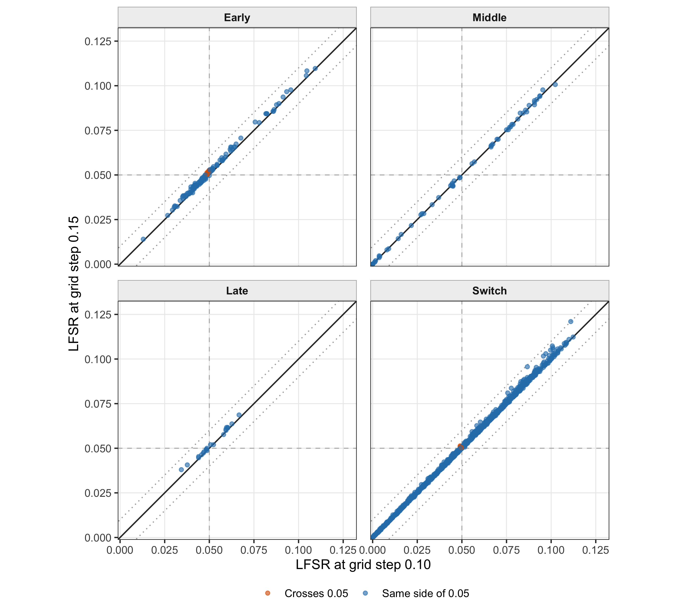
Figure 1. Grid-step sensitivity: 0.10 versus 0.15 at 3,000 posterior draws. Panels contain all baseline-discovery pairs for each category; the discovery population is held fixed.
The points remain close to equality: category-specific mean absolute changes range from 0.0005 to 0.0016. Every pair is within 0.01.
build_comparison_plot(
  comparison_id = "grid_0p10_vs_0p05_M3000",
  x_label = "LFSR at grid step 0.10",
  y_label = "LFSR at grid step 0.05"
)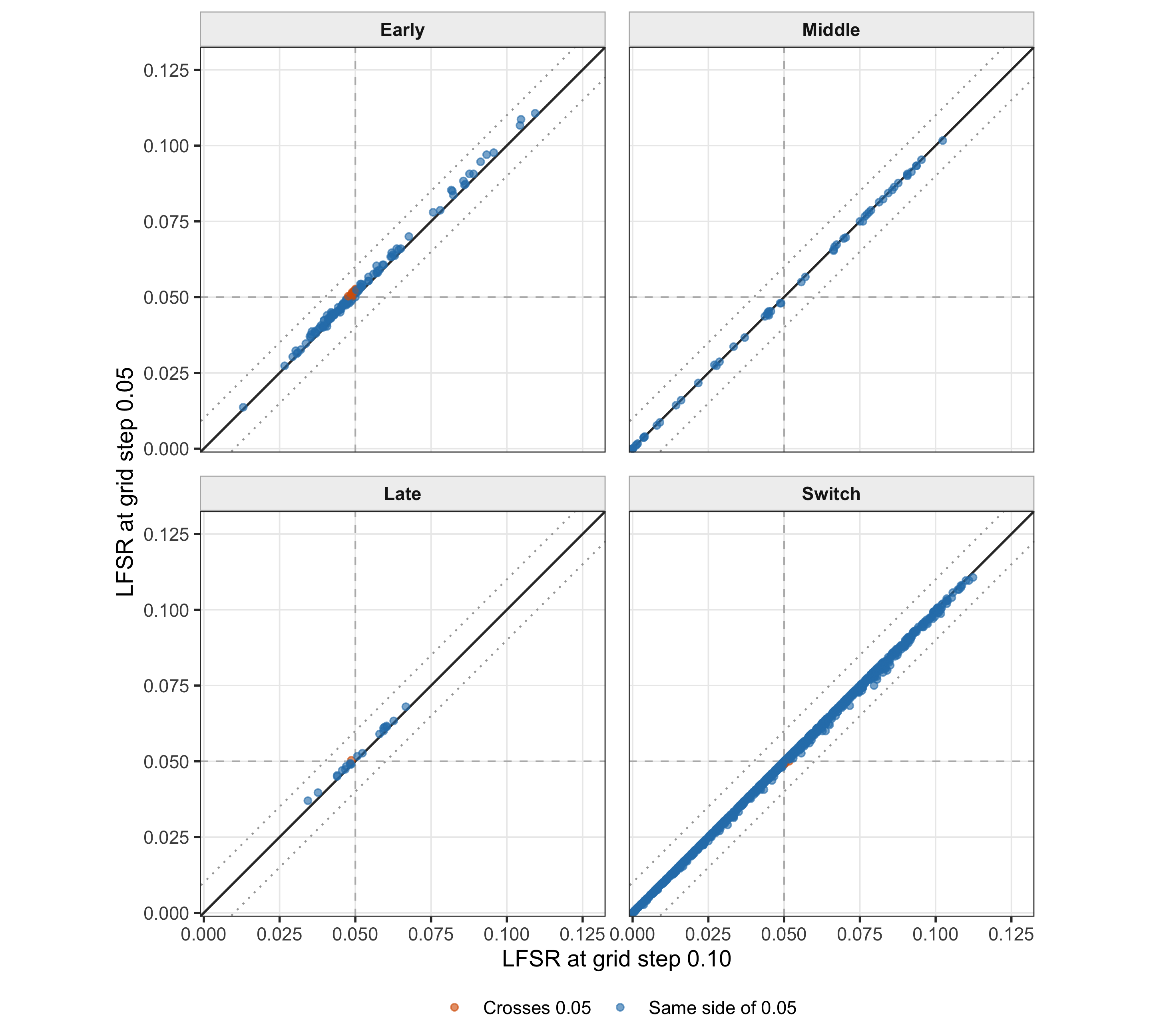
Figure 2. Grid-step sensitivity: 0.10 versus 0.05 at 3,000 posterior draws. Panels contain all baseline-discovery pairs for each category; the discovery population is held fixed.
The finer-grid comparison is at least as stable. Mean absolute changes range from 0.0003 to 0.0016, and every pair is within 0.01. This supports treating grid step 0.10 as adequate for these reported pairs.
build_comparison_plot(
  comparison_id = "M2000_vs_M3000_grid_0p10",
  x_label = "LFSR with 2,000 posterior draws",
  y_label = "LFSR with 3,000 posterior draws"
)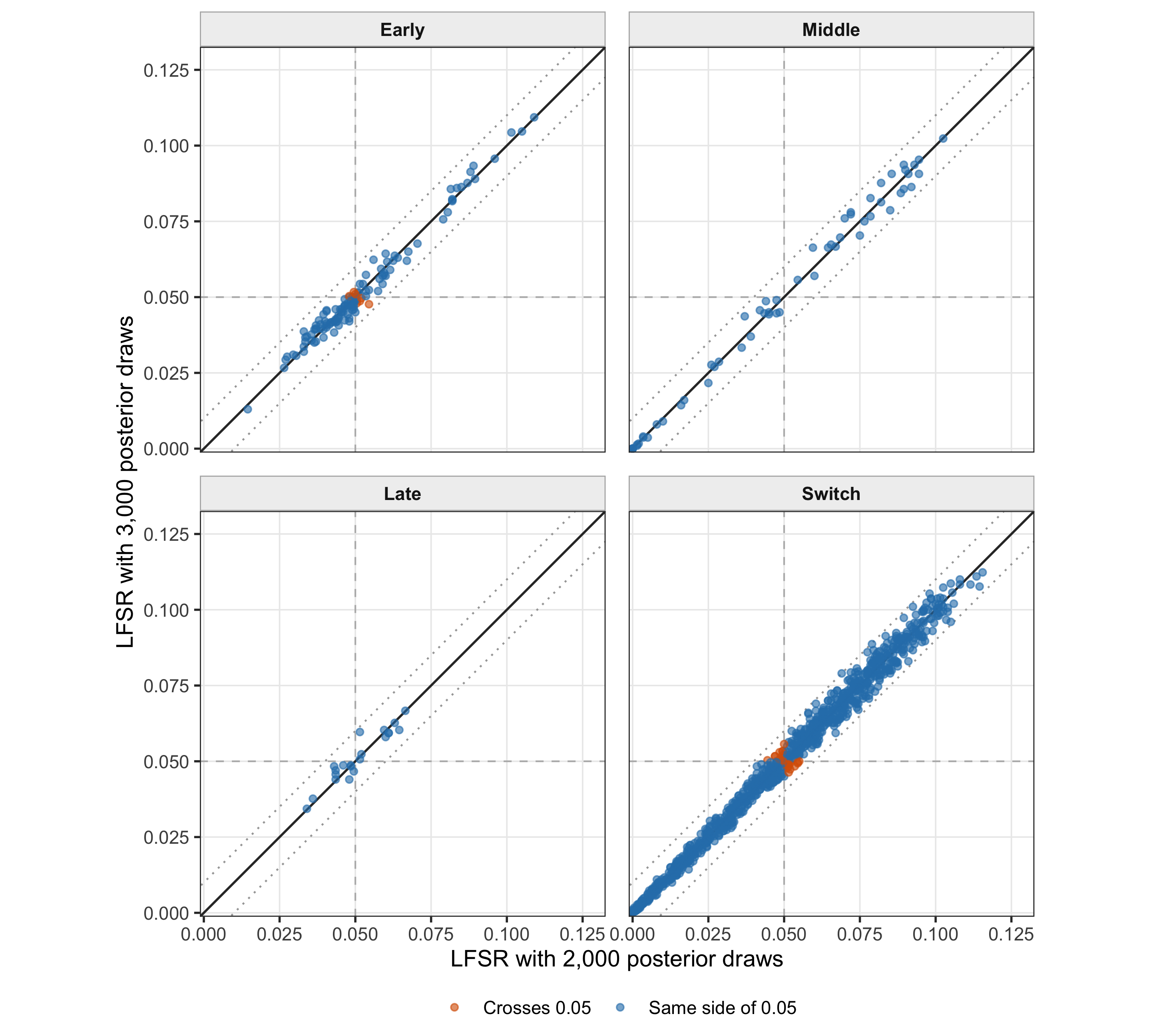
Figure 3. Posterior Monte Carlo sensitivity: 2,000 versus 3,000 nested draws at grid step 0.10. Panels contain all baseline-discovery pairs for each category; columns were deterministically permuted before taking prefixes.
Mean absolute changes range from 0.0020 to 0.0022. Signed mean changes are all within 0.0004 of zero, consistent with Monte Carlo fluctuation rather than a systematic shift.
build_comparison_plot(
  comparison_id = "M3000_vs_M5000_grid_0p10",
  x_label = "LFSR with 3,000 posterior draws",
  y_label = "LFSR with 5,000 posterior draws"
)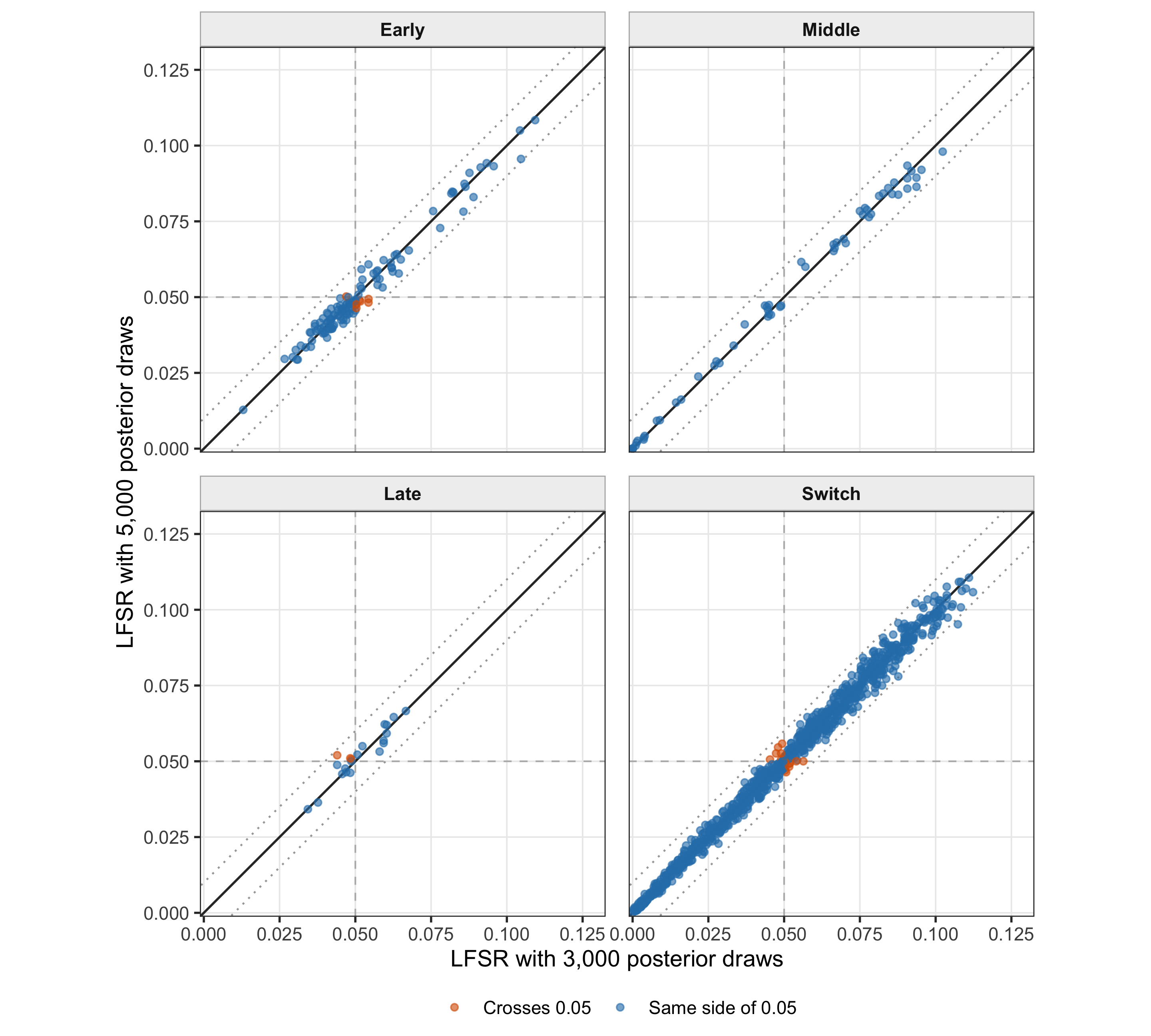
Figure 4. Posterior Monte Carlo sensitivity: 3,000 versus 5,000 nested draws at grid step 0.10. Panels contain all baseline-discovery pairs for each category; columns were deterministically permuted before taking prefixes.
Mean absolute changes are 0.0017–0.0023, with more than 99.8% of pairs within 0.01 in every category. The signed mean changes are all within 0.0007 of zero. Together with the 2,000-versus-3,000 comparison, this supports retaining \(M=3{,}000\) for the reported-pair analysis.
Final numerical choices
- Functional definitions: Early \(t\leq3\); Middle \(3<t<12\); Late \(t\geq12\); Switch threshold 0.25.
- Evaluation grid:
seq(0, 15, by = 0.10). - Posterior Monte Carlo size: 3,000 draws.
- Sensitivity population: all baseline-discovery pairs within each category, held fixed across settings.
- Randomization: pair-specific seed 20260826 plus fitted-pair index, followed by a pair-specific deterministic column permutation for nested prefixes.
- Computation: one R job with two workers; the production posterior-sampling stage took 170.8 seconds.
Reproducibility
The page reads the versioned cache validated by
code/revision_simulations/internal/evaluation_grid_sensitivity/reporting.R.
The numerical cache can be regenerated from the current saved
classifications and BF-adjusted fit with:
Rscript --vanilla \
  code/revision_simulations/internal/evaluation_grid_sensitivity/run_all_category_baseline_discovery_sensitivity.R \
  --num-cores 2 \
  --seed 20260826 \
  --middle-definition open_3_12 \
  --output-id evaluation_grid_mc_all_category_current_fashr0143_20260826
sessionInfo()
#> R version 4.5.1 (2025-06-13)
#> Platform: aarch64-apple-darwin20
#> Running under: macOS Sequoia 15.6.1
#>
#> Matrix products: default
#> BLAS:   /System/Library/Frameworks/Accelerate.framework/Versions/A/Frameworks/vecLib.framework/Versions/A/libBLAS.dylib
#> LAPACK: /Library/Frameworks/R.framework/Versions/4.5-arm64/Resources/lib/libRlapack.dylib;  LAPACK version 3.12.1
#>
#> locale:
#> [1] C.UTF-8/C.UTF-8/C.UTF-8/C/C.UTF-8/C.UTF-8
#>
#> time zone: America/Chicago
#> tzcode source: internal
#>
#> attached base packages:
#> [1] stats     graphics  grDevices utils     datasets  methods   base
#>
#> other attached packages:
#> [1] ggplot2_4.0.3   workflowr_1.7.2
#>
#> loaded via a namespace (and not attached):
#>  [1] gtable_0.3.6       jsonlite_2.0.0     dplyr_1.1.4        compiler_4.5.1
#>  [5] promises_1.5.0     tidyselect_1.2.1   Rcpp_1.1.1-1.1     stringr_1.6.0
#>  [9] git2r_0.36.2       dichromat_2.0-0.1  callr_3.7.6        later_1.4.4
#> [13] jquerylib_0.1.4    scales_1.4.0       yaml_2.3.12        fastmap_1.2.0
#> [17] R6_2.6.1           generics_0.1.4     knitr_1.50         tibble_3.3.0
#> [21] rprojroot_2.1.1    RColorBrewer_1.1-3 bslib_0.9.0        pillar_1.11.1
#> [25] rlang_1.2.0        cachem_1.1.0       stringi_1.8.9      httpuv_1.6.16
#> [29] xfun_0.55          S7_0.2.2           getPass_0.2-4      fs_1.6.6
#> [33] sass_0.4.10        otel_0.2.0         cli_3.6.6          withr_3.0.3
#> [37] magrittr_2.0.5     ps_1.9.1           grid_4.5.1         digest_0.6.39
#> [41] processx_3.8.6     rstudioapi_0.17.1  lifecycle_1.0.5    vctrs_0.7.3
#> [45] evaluate_1.0.5     glue_1.8.1         farver_2.1.2       whisker_0.4.1
#> [49] rmarkdown_2.30     httr_1.4.7         tools_4.5.1        pkgconfig_2.0.3
#> [53] htmltools_0.5.9