Evaluation-grid and posterior Monte Carlo sensitivity
Ziang Zhang
2026-08-26
Last updated: 2026-11-04
Checks: 6 1
Knit directory: coderepo-local/
This reproducible R Markdown analysis was created with workflowr (version 1.7.2). The Checks tab describes the reproducibility checks that were applied when the results were created. The Past versions tab lists the development history.
The R Markdown is untracked by Git. To know which version of the R
Markdown file created these results, you’ll want to first commit it to
the Git repo. If you’re still working on the analysis, you can ignore
this warning. When you’re finished, you can run
wflow_publish to commit the R Markdown file and build the
HTML.
Great job! The global environment was empty. Objects defined in the global environment can affect the analysis in your R Markdown file in unknown ways. For reproduciblity it’s best to always run the code in an empty environment.
The command set.seed(20251109) was run prior to running
the code in the R Markdown file. Setting a seed ensures that any results
that rely on randomness, e.g. subsampling or permutations, are
reproducible.
Great job! Recording the operating system, R version, and package versions is critical for reproducibility.
Nice! There were no cached chunks for this analysis, so you can be confident that you successfully produced the results during this run.
Great job! Using relative paths to the files within your workflowr project makes it easier to run your code on other machines.
Great! You are using Git for version control. Tracking code development and connecting the code version to the results is critical for reproducibility.
The results in this page were generated with repository version bfc8f00. See the Past versions tab to see a history of the changes made to the R Markdown and HTML files.
Note that you need to be careful to ensure that all relevant files for
the analysis have been committed to Git prior to generating the results
(you can use wflow_publish or
wflow_git_commit). workflowr only checks the R Markdown
file, but you know if there are other scripts or data files that it
depends on. Below is the status of the Git repository when the results
were generated:
Ignored files:
    Ignored:    .DS_Store
    Ignored:    .Rhistory
    Ignored:    .Rproj.user/
    Ignored:    Rplots.pdf
    Ignored:    analysis/.DS_Store
    Ignored:    analysis/.Rhistory
    Ignored:    code/.DS_Store
    Ignored:    code/.Rhistory
    Ignored:    code/revision_simulations/.DS_Store
    Ignored:    data/appendixB/
    Ignored:    data/dynamic_eQTL_real/
    Ignored:    data/revision_simulations/
    Ignored:    data/toy_example/
    Ignored:    output/dynamic_eQTL_real/
    Ignored:    output/pdf/
    Ignored:    output/playwright/
    Ignored:    output/revision_simulations/
    Ignored:    scripts/

Untracked files:
    Untracked:  analysis/balanced_variant_thinning.rmd
    Untracked:  analysis/enhancer_enrichment.rmd
    Untracked:  analysis/evaluation_grid_mc_sensitivity.rmd
    Untracked:  analysis/functional_testing_simulation.rmd
    Untracked:  analysis/matched_fash_linear_real_data.rmd
    Untracked:  code/revision_simulations/internal/appendix_c1_j1000/
    Untracked:  code/revision_simulations/internal/per_unit_enhancer_enrichment/
    Untracked:  code/revision_simulations/internal/per_unit_expression_correlation/compare_corshrink_versions.R
    Untracked:  code/revision_simulations/internal/per_unit_expression_correlation/diagnose_discordant_calls.R
    Untracked:  code/revision_simulations/internal/per_unit_expression_correlation/diagnose_smooth_mismatch.R
    Untracked:  code/revision_simulations/internal/per_unit_expression_correlation/extract_perunit_lfdr.R
    Untracked:  code/revision_simulations/internal/per_unit_expression_correlation/plot_call_venns.R
    Untracked:  code/revision_simulations/internal/per_unit_expression_correlation/plot_class_variograms.R
    Untracked:  code/revision_simulations/internal/per_unit_expression_correlation/plot_corshrink_result.R
    Untracked:  code/revision_simulations/internal/per_unit_expression_correlation/plot_corshrink_versions.R
    Untracked:  code/revision_simulations/internal/per_unit_expression_correlation/plot_cs_vs_diagonal.R
    Untracked:  code/revision_simulations/internal/per_unit_expression_correlation/plot_day0_day1_distribution.R
    Untracked:  code/revision_simulations/internal/per_unit_expression_correlation/plot_mechanism_summary.R
    Untracked:  code/revision_simulations/internal/per_unit_expression_correlation/plot_perunit_variogram.R
    Untracked:  code/revision_simulations/internal/per_unit_expression_correlation/plot_strober_concordance.R
    Untracked:  code/revision_simulations/internal/per_unit_expression_correlation/plot_three_models.R
    Untracked:  code/revision_simulations/internal/per_unit_expression_correlation/prepare_reference_sets.R
    Untracked:  code/revision_simulations/internal/per_unit_expression_correlation/prototype_corshrink.R
    Untracked:  code/revision_simulations/internal/per_unit_expression_correlation/recover_design_factor.R
    Untracked:  code/revision_simulations/internal/per_unit_expression_correlation/test_corshrink_reimplementation.R
    Untracked:  code/revision_simulations/internal/posterior_interval_coverage/
    Untracked:  code/revision_simulations/internal/r3_stage1_method_comparison/plot_pi0_before_after.py

Unstaged changes:
    Modified:   analysis/about.Rmd
    Modified:   analysis/appendixB.rmd
    Modified:   analysis/dynamic_eQTL_real.rmd
    Deleted:    analysis/dynamic_eQTL_real_cl.rmd
    Deleted:    analysis/dynamic_eQTL_real_full.rmd
    Modified:   analysis/index.Rmd
    Modified:   analysis/license.Rmd
    Modified:   analysis/nonlinear_dynamic_eQTL_real.Rmd
    Deleted:    analysis/nonlinear_dynamic_eQTL_real_cl.Rmd
    Deleted:    analysis/nonlinear_dynamic_eQTL_real_full.rmd
    Deleted:    analysis/revision_balanced_variant_thinning.rmd
    Deleted:    analysis/revision_combined_spiky_genotype_simulation.rmd
    Deleted:    analysis/revision_correlated_error_simulation.rmd
    Deleted:    analysis/revision_enhancer_enrichment.rmd
    Deleted:    analysis/revision_enhancer_enrichment_cl.rmd
    Deleted:    analysis/revision_functional_testing_simulation.rmd
    Deleted:    analysis/revision_genotype_level_simulation.rmd
    Deleted:    analysis/revision_internal_baseline_ld_variant_enrichment.rmd
    Deleted:    analysis/revision_internal_correlated_likelihood_sensitivity.rmd
    Deleted:    analysis/revision_internal_correlated_permutation_discoveries.rmd
    Deleted:    analysis/revision_internal_evaluation_grid_mc_sensitivity.rmd
    Deleted:    analysis/revision_internal_evaluation_grid_mc_sensitivity_middle_4_11.rmd
    Deleted:    analysis/revision_internal_fash_cl_manuscript_impact.rmd
    Deleted:    analysis/revision_internal_fash_cl_variant_enrichment_comparison.rmd
    Deleted:    analysis/revision_internal_fash_discovery_variant_count.rmd
    Deleted:    analysis/revision_internal_fash_knockoff.rmd
    Deleted:    analysis/revision_internal_fash_linear_real_data_ablation.rmd
    Deleted:    analysis/revision_internal_fash_temporal_class_enhancer_enrichment.rmd
    Deleted:    analysis/revision_internal_fashr_correlated_observation_model.rmd
    Deleted:    analysis/revision_internal_mashr_mean_z_null_correlation.rmd
    Deleted:    analysis/revision_internal_matched_fash_linear_real_data.rmd
    Deleted:    analysis/revision_internal_matched_fash_linear_real_data_cl.rmd
    Deleted:    analysis/revision_internal_observational_null_set_pilot.rmd
    Deleted:    analysis/revision_internal_one_variant_per_gene_refit.rmd
    Deleted:    analysis/revision_internal_r1_normality_assumption.rmd
    Deleted:    analysis/revision_internal_r3_full_calibration.rmd
    Deleted:    analysis/revision_internal_r3_ideal_gaussian_measurement.rmd
    Deleted:    analysis/revision_internal_r3_truth_specification_pilot.rmd
    Deleted:    analysis/revision_internal_real_genotype_simulation.rmd
    Deleted:    analysis/revision_internal_roadmap_enhancer_exploration.rmd
    Deleted:    analysis/revision_internal_small_m_clean_working_null_sensitivity.rmd
    Deleted:    analysis/revision_internal_small_m_matched_null_eb_sensitivity.rmd
    Deleted:    analysis/revision_internal_targeted_broad_calibration.rmd
    Deleted:    analysis/revision_internal_temporal_class_roadmap_enrichment.rmd
    Deleted:    analysis/revision_internal_three_likelihood_comparison.rmd
    Deleted:    analysis/revision_internal_twenty_variant_per_gene_refit.rmd
    Deleted:    analysis/revision_internal_variant_annotation_enrichment.rmd
    Deleted:    analysis/revision_internal_zero_intercept_correlation.rmd
    Deleted:    analysis/revision_ld_tagging_switch_example.rmd
    Deleted:    analysis/toy_example.rmd
    Modified:   code/figure_exports/pages/export_revision_balanced_variant_thinning.R
    Modified:   code/figure_exports/pages/export_revision_enhancer_enrichment.R
    Modified:   code/figure_exports/pages/export_revision_functional_testing_simulation.R
    Modified:   code/figure_exports/pages/export_revision_internal_evaluation_grid_mc_sensitivity.R
    Modified:   code/figure_exports/pages/export_revision_internal_matched_fash_linear_real_data.R
    Modified:   code/revision_simulations/r5_one_variant_per_gene/reporting.R
Note that any generated files, e.g. HTML, png, CSS, etc., are not included in this status report because it is ok for generated content to have uncommitted changes.
There are no past versions. Publish this analysis with
wflow_publish() to start tracking its development.
Overview
We assess the sensitivity of the dynamic eQTL functional
classifications (Early, Middle, Late, and Switch) to the evaluation-grid
step size and the number of posterior Monte Carlo draws. The main
analysis uses evaluation-grid step 0.10 on \([0, 15]\) and \(M
= 3{,}000\) posterior draws. Here we compare the resulting
lfsr values for the discovered gene–variant pairs in each
category against alternative grid steps (0.15 and
0.05 at \(M = 3{,}000\))
and alternative Monte Carlo sample sizes (\(M
= 2{,}000\) and \(M = 5{,}000\)
at grid step 0.10).
For posterior trajectory draw \(\beta^{(m)}(t)\), the four functional statistics are
\[ \begin{aligned} T_{\mathrm{early}}^{(m)} &= \sup_{t\leq3}|\beta^{(m)}(t)|-\sup_{t>3}|\beta^{(m)}(t)|,\\ T_{\mathrm{middle}}^{(m)} &= \sup_{3<t<12}|\beta^{(m)}(t)| -\sup_{t\leq3\;\mathrm{or}\;t\geq12}|\beta^{(m)}(t)|,\\ T_{\mathrm{late}}^{(m)} &= \sup_{t\geq12}|\beta^{(m)}(t)|-\sup_{t<12}|\beta^{(m)}(t)|,\\ T_{\mathrm{switch}}^{(m)} &= \min\!\left\{\sup_t \beta^{(m)}(t),-\inf_t \beta^{(m)}(t)\right\}-0.25, \end{aligned} \]
and the local false sign rate for category \(c\) is estimated by
\[ \widehat{\mathrm{lfsr}}_c =\frac{1}{M}\sum_{m=1}^{M}I\!\left\{T_c^{(m)}\leq0\right\}. \]
category_display_names <- c(
  early = "Early",
  middle = "Middle",
  late = "Late",
  switch = "Switch"
)

population_table <- data.frame(
  Category = unname(category_display_names[population_summary$category]),
  Definition = c(
    "Strongest effect during the first three days (t <= 3)",
    "Strongest effect in the middle window (3 < t < 12)",
    "Strongest effect during the last four days (t >= 12)",
    "Positive and negative excursions both exceed 0.25"
  ),
  `Discovered pairs` = population_summary$n_pairs,
  `Unique genes` = population_summary$n_genes,
  check.names = FALSE
)

knitr::kable(
  population_table,
  align = c("l", "l", "r", "r"),
  caption = "Table 1. Dynamic eQTL functional categories and numbers of discovered pairs and genes (cumulative FSR <= 0.05 at grid step 0.10 and 3,000 posterior draws)."
)| Category | Definition | Discovered pairs | Unique genes |
|---|---|---|---|
| Early | Strongest effect during the first three days (t <= 3) | 126 | 8 |
| Middle | Strongest effect in the middle window (3 < t < 12) | 58 | 14 |
| Late | Strongest effect during the last four days (t >= 12) | 21 | 11 |
| Switch | Positive and negative excursions both exceed 0.25 | 981 | 250 |
library(ggplot2)

build_comparison_data <- function(comparison_id) {
  comparison_spec <- configuration$comparisons[
    configuration$comparisons$comparison_id == comparison_id,
    ,
    drop = FALSE
  ]
  if (nrow(comparison_spec) != 1L) {
    stop("The requested comparison is not uniquely specified.")
  }

  x_rows <- pair_lfsr[
    pair_lfsr$setting_id == comparison_spec$x_setting_id,
    c("category", "pair_id", "gene_symbol", "lfsr"),
    drop = FALSE
  ]
  y_rows <- pair_lfsr[
    pair_lfsr$setting_id == comparison_spec$y_setting_id,
    c("category", "pair_id", "lfsr"),
    drop = FALSE
  ]
  names(x_rows)[names(x_rows) == "lfsr"] <- "x_lfsr"
  names(y_rows)[names(y_rows) == "lfsr"] <- "y_lfsr"

  plot_data <- merge(
    x_rows,
    y_rows,
    by = c("category", "pair_id"),
    all = FALSE,
    sort = FALSE
  )

  plot_data$category_panel <- factor(
    plot_data$category,
    levels = category_order,
    labels = unname(category_display_names[category_order])
  )
  plot_data
}

build_comparison_plot <- function(comparison_id, x_label, y_label) {
  plot_data <- build_comparison_data(comparison_id)

  ggplot(plot_data, aes(x = x_lfsr, y = y_lfsr)) +
    geom_abline(
      intercept = c(-0.01, 0.01),
      slope = 1,
      color = "grey65",
      linewidth = 0.45,
      linetype = "dotted"
    ) +
    geom_abline(
      intercept = 0,
      slope = 1,
      color = "grey20",
      linewidth = 0.55
    ) +
    geom_vline(
      xintercept = 0.05,
      color = "grey72",
      linewidth = 0.4,
      linetype = "dashed"
    ) +
    geom_hline(
      yintercept = 0.05,
      color = "grey72",
      linewidth = 0.4,
      linetype = "dashed"
    ) +
    geom_point(
      color = "#1B9E77",
      alpha = 0.65,
      size = 1.4
    ) +
    facet_wrap(~category_panel, ncol = 2) +
    scale_x_continuous(
      limits = c(0, 0.13),
      breaks = c(0, 0.05, 0.10),
      labels = c("0", "0.05", "0.10"),
      expand = expansion(mult = c(0.01, 0.02))
    ) +
    scale_y_continuous(
      limits = c(0, 0.13),
      breaks = c(0, 0.05, 0.10),
      labels = c("0", "0.05", "0.10"),
      expand = expansion(mult = c(0.01, 0.02))
    ) +
    coord_equal() +
    labs(
      x = x_label,
      y = y_label
    ) +
    theme_minimal(base_size = 12) +
    theme(
      panel.grid.minor = element_blank(),
      panel.grid.major = element_line(color = "grey92", linewidth = 0.35),
      strip.background = element_blank(),
      strip.text = element_text(face = "bold", size = 12),
      panel.spacing = grid::unit(1.0, "lines")
    )
}
Evaluation-grid sensitivity
We first compare evaluation-grid step 0.10 against a
coarser grid (0.15) and a finer grid (0.05),
holding the number of posterior draws fixed at \(M = 3{,}000\). In all plots below, the
solid diagonal indicates equality and the dotted lines mark an absolute
lfsr difference of 0.01.
build_comparison_plot(
  comparison_id = "grid_0p10_vs_0p05_M3000",
  x_label = "lfsr at grid step 0.10",
  y_label = "lfsr at grid step 0.05"
)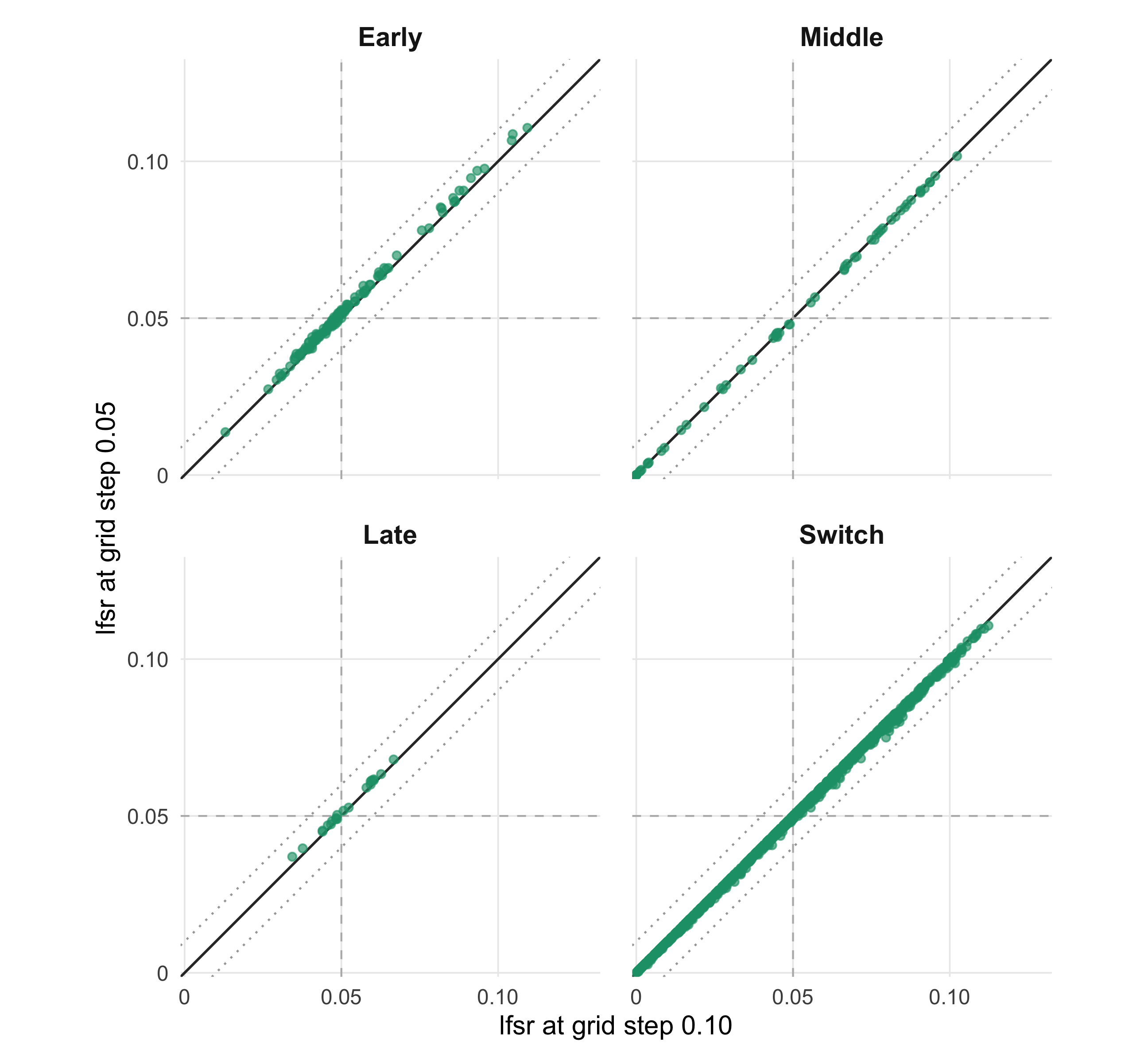
Figure 1. Evaluation-grid sensitivity: step 0.10 versus 0.05 at 3,000 posterior draws across the four functional categories.
build_comparison_plot(
  comparison_id = "grid_0p10_vs_0p15_M3000",
  x_label = "lfsr at grid step 0.10",
  y_label = "lfsr at grid step 0.15"
)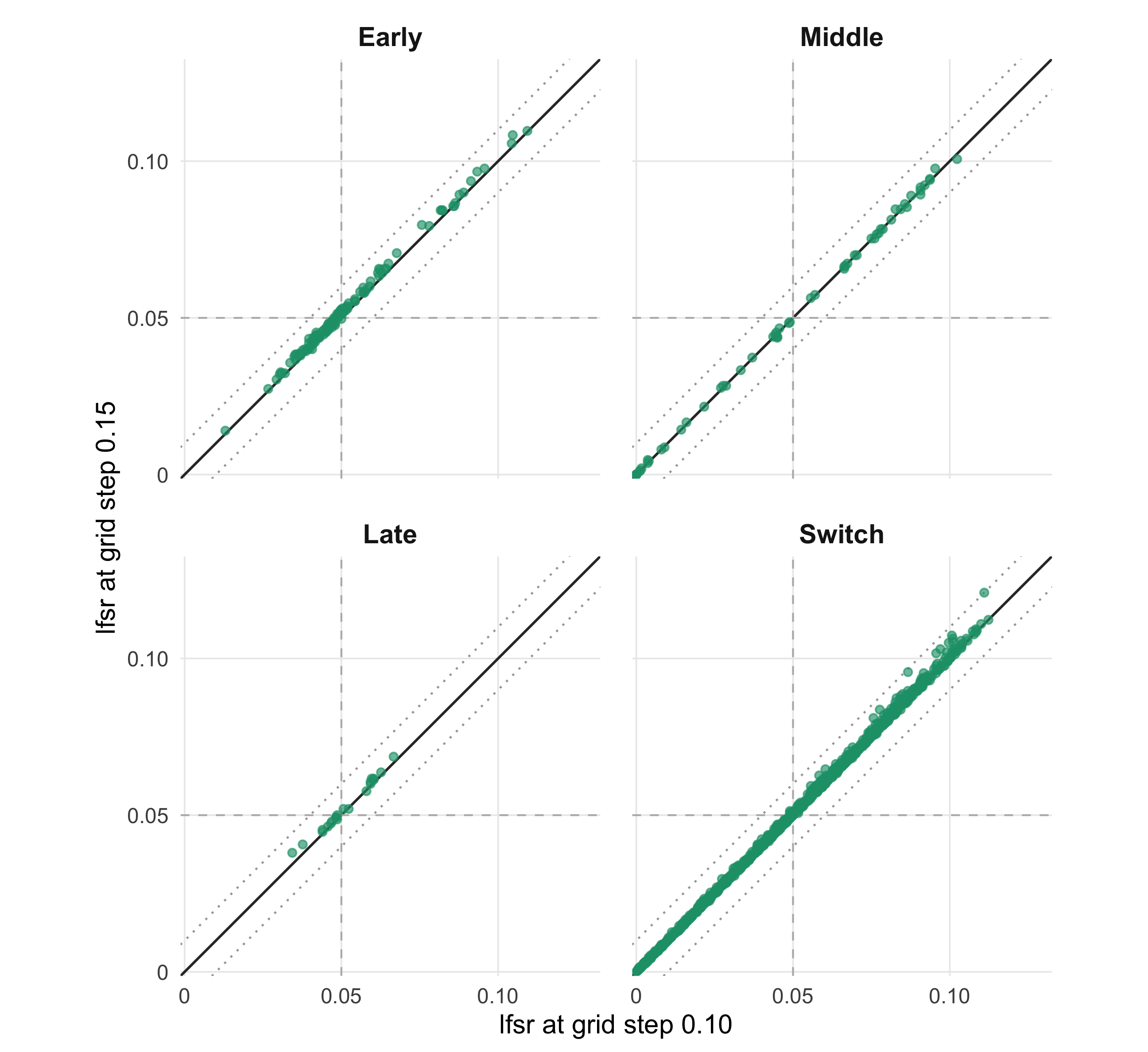
Figure 2. Evaluation-grid sensitivity: step 0.10 versus 0.15 at 3,000 posterior draws across the four functional categories.
Across the four categories, mean absolute lfsr
differences relative to step 0.10 range from
0.0003 to 0.0016 for step 0.05
and from 0.0005 to 0.0016 for step
0.15, with every pair differing by at most
0.01.
Posterior Monte Carlo sensitivity
Next, we compare \(M = 3{,}000\)
posterior draws against \(M = 5{,}000\)
and \(M = 2{,}000\) draws at
evaluation-grid step 0.10.
build_comparison_plot(
  comparison_id = "M3000_vs_M5000_grid_0p10",
  x_label = "lfsr with 3,000 draws",
  y_label = "lfsr with 5,000 draws"
)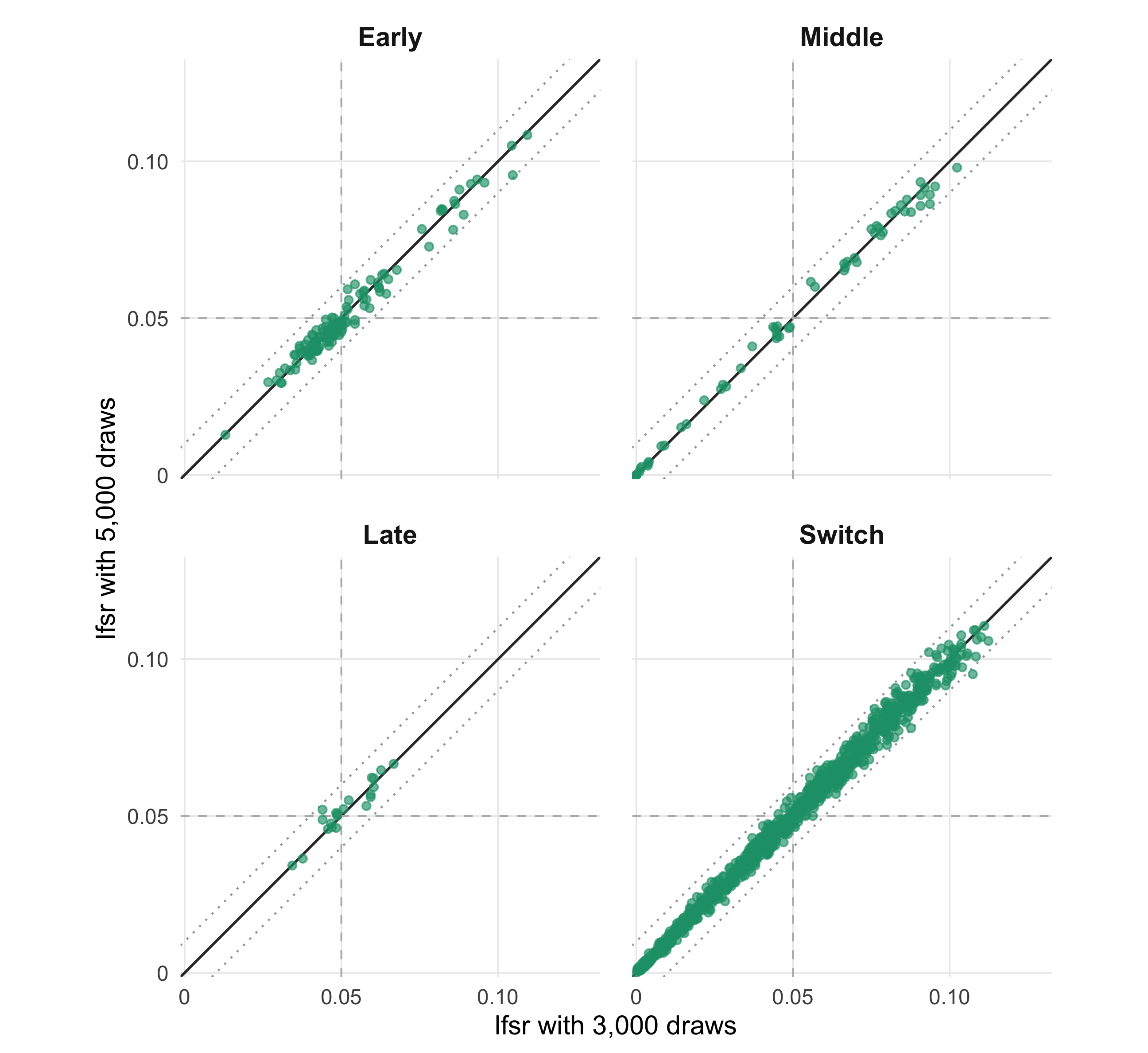
Figure 3. Posterior Monte Carlo sensitivity: 3,000 versus 5,000 posterior draws at evaluation-grid step 0.10.
build_comparison_plot(
  comparison_id = "M2000_vs_M3000_grid_0p10",
  x_label = "lfsr with 2,000 draws",
  y_label = "lfsr with 3,000 draws"
)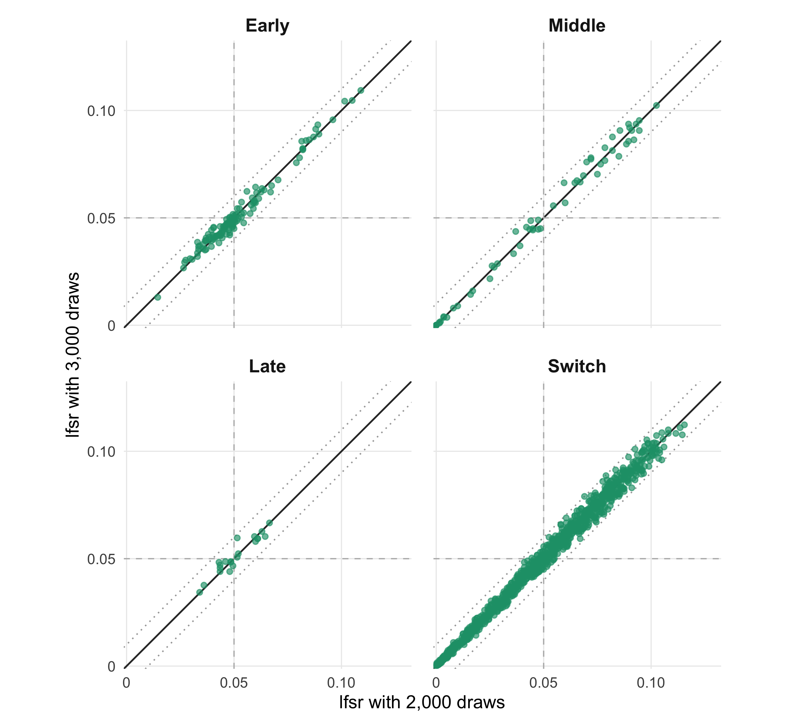
Figure 4. Posterior Monte Carlo sensitivity: 2,000 versus 3,000 posterior draws at evaluation-grid step 0.10.
Across categories, mean absolute lfsr differences are
0.0017–0.0023 between 3,000 and 5,000 draws
(with more than 99.8% of pairs differing by at most 0.01)
and 0.0020–0.0022 between 2,000 and 3,000
draws.
Reproducibility
The sensitivity analysis can be reproduced with:
Rscript --vanilla \
  code/revision_simulations/internal/evaluation_grid_sensitivity/run_all_category_baseline_discovery_sensitivity.R \
  --num-cores 2 \
  --seed 20260826 \
  --middle-definition open_3_12 \
  --output-id evaluation_grid_mc_all_category_current_fashr0143_20260826
sessionInfo()
#> R version 4.5.1 (2025-06-13)
#> Platform: aarch64-apple-darwin20
#> Running under: macOS Sequoia 15.6.1
#>
#> Matrix products: default
#> BLAS:   /System/Library/Frameworks/Accelerate.framework/Versions/A/Frameworks/vecLib.framework/Versions/A/libBLAS.dylib
#> LAPACK: /Library/Frameworks/R.framework/Versions/4.5-arm64/Resources/lib/libRlapack.dylib;  LAPACK version 3.12.1
#>
#> locale:
#> [1] en_CA/en_CA/en_CA/C/en_CA/en_CA
#>
#> time zone: America/Chicago
#> tzcode source: internal
#>
#> attached base packages:
#> [1] stats     graphics  grDevices utils     datasets  methods   base
#>
#> other attached packages:
#> [1] ggplot2_4.0.3
#>
#> loaded via a namespace (and not attached):
#>  [1] gtable_0.3.6       jsonlite_2.0.0     dplyr_1.1.4        compiler_4.5.1
#>  [5] promises_1.5.0     tidyselect_1.2.1   Rcpp_1.1.1-1.1     stringr_1.6.0
#>  [9] git2r_0.36.2       dichromat_2.0-0.1  later_1.4.4        jquerylib_0.1.4
#> [13] scales_1.4.0       yaml_2.3.12        fastmap_1.2.0      R6_2.6.1
#> [17] generics_0.1.4     workflowr_1.7.2    knitr_1.50         tibble_3.3.0
#> [21] rprojroot_2.1.1    bslib_0.9.0        pillar_1.11.1      RColorBrewer_1.1-3
#> [25] rlang_1.2.0        cachem_1.1.0       stringi_1.8.9      httpuv_1.6.16
#> [29] xfun_0.55          S7_0.2.2           fs_1.6.6           sass_0.4.10
#> [33] otel_0.2.0         cli_3.6.6          withr_3.0.3        magrittr_2.0.5
#> [37] digest_0.6.39      grid_4.5.1         rstudioapi_0.17.1  lifecycle_1.0.5
#> [41] vctrs_0.7.3        evaluate_1.0.5     glue_1.8.1         farver_2.1.2
#> [45] rmarkdown_2.30     tools_4.5.1        pkgconfig_2.0.3    htmltools_0.5.9