Figure 3: GPs associated with T-cell activation

workflowr

• Summary
• Checks
• Past versions

Last updated: 2026-07-02

Checks: 5 1

Knit directory: immgenT-GP-analysis/analysis/

This reproducible R Markdown analysis was created with workflowr (version 1.7.2). The Checks tab describes the reproducibility checks that were applied when the results were created. The Past versions tab lists the development history.

---

Environment: empty

Great job! The global environment was empty. Objects defined in the global environment can affect the analysis in your R Markdown file in unknown ways. For reproduciblity it’s best to always run the code in an empty environment.

Seed: set.seed(1)

The command set.seed(1) was run prior to running the code in the R Markdown file. Setting a seed ensures that any results that rely on randomness, e.g. subsampling or permutations, are reproducible.

Session information: recorded

Great job! Recording the operating system, R version, and package versions is critical for reproducibility.

Cache: none

Nice! There were no cached chunks for this analysis, so you can be confident that you successfully produced the results during this run.

File paths: relative

Great job! Using relative paths to the files within your workflowr project makes it easier to run your code on other machines.

Repository version: no version control

Tracking code development and connecting the code version to the results is critical for reproducibility. To start using Git, open the Terminal and type git init in your project directory.

---

This project is not being versioned with Git. To obtain the full reproducibility benefits of using workflowr, please see ?wflow_start.

---

All panels are produced by script-refactor/Figure3.R, which shares its curated GP set with Figure S3 via code-refactor/R/activation_shared_setup.R. The code below is shown for reference (not re-executed on this page); the images are its pre-rendered output.

Setup

Data loading, shared across all panels below.

# Figure 3. GPs associated with T-cell activation.
#
# Panels produced (see figures/Figure3_Activation/Figure3_caption.md for the
# full caption text -- lettered a-e there, but relettered c-g in the final
# figures/final-selected/bits/Figure 3/ bundle; this script uses the final
# c-g lettering to match):
#   3c  Standardized mean difference (d) in GP loading, activated vs resting,
#       CD4 (x) vs CD8 (y); curated GPs colored by semantic group and labeled.
#   3d  GP-gene signature network: each curated GP linked to its top 5
#       positively/negatively regulated genes.
#   3e  Bipartite TF-GP network for the curated activation GPs.
#   3f  Heatmap of log2FC in mean GP loading across experimental conditions,
#       for activated CD4/CD8 cells.
#   3g  Heatmap of mean GP loading per Level-2 sub-lineage, across the 7
#       T-cell lineages.
#
# Source: ported from script/Figure_Activation.R, which also produced the
# Figure S3 panels (see FigureS3.R) from the same curated GP set and cell
# groupings -- that shared setup now lives in
# code-refactor/R/activation_shared_setup.R, sourced by both scripts.

library(ggplot2)
library(ggrepel)
library(dplyr)
library(tidygraph)
library(ggraph)
library(pheatmap)
library(scales)

data_path <- "data/"
figure_path <- "figure-refactor/Figure 3/"
source("code-refactor/R/plot_utils.R") # scale_cols()
source("code-refactor/R/tf_network.R") # optimize_bipartite_order(), plot_tf_gp_network_v2()

# ============================================================
# Load data
# ============================================================
L_pm_filtered <- readRDS(paste0(data_path, "L_pm_filtered.rds"))
colnames(L_pm_filtered) <- paste0("GP", seq_len(ncol(L_pm_filtered)))
F_pm_filtered <- readRDS(paste0(data_path, "F_pm_filtered.rds"))
colnames(F_pm_filtered) <- paste0("GP", seq_len(ncol(F_pm_filtered)))
seurat_meta <- readRDS(paste0(data_path, "igt1_96_withtotalvi20260206_clean_ADTonly.Rds"))@meta.data
seurat_meta_filtered <- seurat_meta[rownames(L_pm_filtered), ]

source("code-refactor/R/activation_shared_setup.R")

(3c) Activation effect, CD4 vs. CD8

# ============================================================
# 3a: Standardized mean difference, activated vs resting, CD4 vs CD8
# ============================================================
d_thr <- 0.15
ratio_cutoff <- 3

GP_activation_summary <- diff_factors_merged %>%
  dplyr::inner_join(d_factors_merged %>% dplyr::select(SYMBOL, d_CD4, d_CD8), by = "SYMBOL") %>%
  dplyr::mutate(Ratio_CD8_CD4 = mean_change_loadings_CD8 / mean_change_loadings_CD4) %>%
  dplyr::select(GP = SYMBOL, mean_change_loadings_CD4, mean_change_loadings_CD8, AveExpr_CD4, AveExpr_CD8, d_CD4, d_CD8, Ratio_CD8_CD4)

# Colour every GP using the same four-category rule (ratio + sign + magnitude
# gate via d_thr). Curated GPs (GPs_of_interest) override with their fixed
# manual highlight_colors; non-curated GPs are classified automatically.
# Only the curated GPs are labelled, to keep the plot readable.
manual_curated_df <- GP_activation_summary %>%
  dplyr::mutate(
    auto_color = dplyr::case_when(
      abs(Ratio_CD8_CD4) > ratio_cutoff & abs(d_CD8) > d_thr ~ "darkorange2",
      abs(Ratio_CD8_CD4) < 1 / ratio_cutoff & abs(d_CD4) > d_thr ~ "blue",
      abs(Ratio_CD8_CD4) > 1 / ratio_cutoff & abs(Ratio_CD8_CD4) < ratio_cutoff & d_CD4 > d_thr & d_CD8 > d_thr ~ "darkred",
      abs(Ratio_CD8_CD4) > 1 / ratio_cutoff & abs(Ratio_CD8_CD4) < ratio_cutoff & d_CD4 < -d_thr & d_CD8 < -d_thr ~ "darkgreen",
      TRUE ~ "black"
    ),
    point_color = ifelse(GP %in% GPs_of_interest, highlight_colors[GP], auto_color)
  )

p_3a <- ggplot(manual_curated_df, aes(x = d_CD4, y = d_CD8)) +
  geom_abline(slope = 1, intercept = 0, linetype = "dashed", color = "red") +
  geom_hline(yintercept = 0, linetype = "dashed", color = "blue") +
  geom_vline(xintercept = 0, linetype = "dashed", color = "blue") +
  geom_point(aes(color = point_color), size = 2) +
  ggrepel::geom_text_repel(
    data = filter(manual_curated_df, GP %in% GPs_of_interest),
    aes(label = GP, color = point_color),
    max.overlaps = Inf, size = 3.5, box.padding = 0.35, point.padding = 0.5, segment.color = "grey50"
  ) +
  scale_color_identity() +
  # Signed (pseudo-)log axes: d is signed, so a plain log drops negatives/zeros.
  scale_x_continuous(trans = scales::pseudo_log_trans(sigma = 0.15), breaks = c(-1, -0.5, -0.2, -0.1, 0, 0.1, 0.2, 0.5, 1)) +
  scale_y_continuous(trans = scales::pseudo_log_trans(sigma = 0.15), breaks = c(-1, -0.5, -0.2, -0.1, 0, 0.1, 0.2, 0.5, 1)) +
  coord_equal(xlim = c(-1.6, 1.6), ylim = c(-1.6, 1.6)) +
  labs(
    x = "Standardized Mean Difference (d) for CD4 Activated vs Resting",
    y = "Standardized Mean Difference (d) for CD8 Activated vs Resting",
    title = "GPs colored by semantic category (curated set labeled)"
  ) +
  theme_minimal()
ggsave(filename = paste0(figure_path, "3c.pdf"), plot = p_3a, width = 8, height = 7)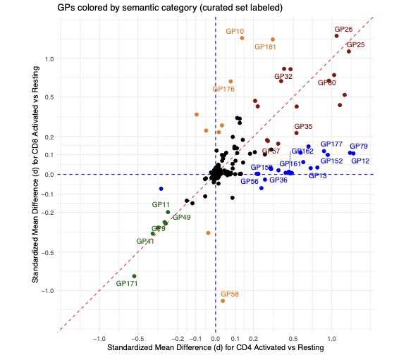

Fig. 3c. Standardized mean difference (d) in GP loading between activated and resting cells, comparing CD4 (x-axis) and CD8 (y-axis); for each GP, d is the activated-minus-resting difference in mean loading divided by that GP’s loading SD pooled over all activated and resting CD4/CD8 cells. Points are colored based on whether they are highly up-regulated in both CD4/CD8 activation, down-regulated in both, or only in CD4 or CD8 activation; GPs not meeting these criteria are shown in black, and only the curated set is labeled.

(3d) GP-gene signature network

# ============================================================
# 3b: GP-gene signature network
# ============================================================
set.seed(42)
F_pm_filtered_norm_subset <- F_pm_filtered_norm[, GPs_of_interest, drop = FALSE]
top_5_pos <- apply(F_pm_filtered_norm_subset, 2, function(x) {
  idx <- order(abs(x), decreasing = TRUE)[1:5]
  idx <- idx[x[idx] > 0]
  names(x)[idx]
})
top_5_neg <- apply(F_pm_filtered_norm_subset, 2, function(x) {
  idx <- order(abs(x), decreasing = TRUE)[1:5]
  idx <- idx[x[idx] < 0]
  names(x)[idx]
})
names(top_5_pos) <- GPs_of_interest
names(top_5_neg) <- GPs_of_interest

pos_edges <- stack(top_5_pos) %>% dplyr::rename(Gene = values, GP = ind) %>% dplyr::mutate(Type = "Positive", Color = "red")
neg_edges <- stack(top_5_neg) %>% dplyr::rename(Gene = values, GP = ind) %>% dplyr::mutate(Type = "Negative", Color = "blue")
all_edges <- dplyr::bind_rows(pos_edges, neg_edges) %>% dplyr::filter(Gene != "" & !is.na(Gene))
all_edges_sorted <- all_edges %>% dplyr::arrange(Type, GP, Gene)

gp_group_df <- data.frame(
  name = names(highlight_colors),
  ManualGroup = dplyr::case_when(
    highlight_colors == "blue" ~ "CD4 only",
    highlight_colors == "darkorange2" ~ "CD8 only",
    highlight_colors == "darkgreen" ~ "both down",
    highlight_colors == "darkred" ~ "both up",
  )
)
manual_colors_palette <- c("CD4 only" = "blue", "CD8 only" = "darkorange2", "both down" = "darkgreen", "both up" = "darkred", "Gene" = "#666666")

graph <- tidygraph::as_tbl_graph(all_edges_sorted) %>%
  tidygraph::activate(nodes) %>%
  dplyr::mutate(
    NodeGroup = ifelse(name %in% all_edges$GP, "GP", "Gene"),
    Importance = tidygraph::centrality_degree()
  ) %>%
  dplyr::left_join(gp_group_df, by = "name") %>%
  dplyr::mutate(
    ColorGroup = ifelse(NodeGroup == "Gene", "Gene", ManualGroup),
    gp_label = ifelse(NodeGroup == "GP", name, "")
  )

set.seed(2)
p_3b <- ggraph(graph, layout = "stress") +
  geom_edge_link(aes(color = Color), alpha = 0.4, width = 0.6) +
  geom_node_point(aes(filter = (NodeGroup == "Gene"), color = ColorGroup), shape = 16, size = 2, alpha = 0.8) +
  geom_node_point(aes(filter = (NodeGroup == "GP"), color = ColorGroup), shape = 15, size = 10, alpha = 0.7) +
  geom_node_text(aes(filter = (NodeGroup == "GP"), label = gp_label), color = "white", fontface = "bold", size = 3) +
  geom_node_text(aes(filter = (NodeGroup == "Gene"), label = name), repel = TRUE, size = 2.5, color = "black", max.overlaps = 20) +
  scale_edge_color_identity() +
  scale_color_manual(name = "GP Types", values = manual_colors_palette, breaks = c("CD4 only", "CD8 only", "both down", "both up")) +
  theme_void() +
  labs(title = "GP-Gene Signature Network", subtitle = "Nodes colored by manual GP classification", caption = "Red edges: Positive | Blue edges: Negative") +
  theme(legend.position = "bottom", legend.title = element_text(face = "bold"), plot.margin = margin(10, 10, 10, 10)) +
  guides(color = guide_legend(override.aes = list(size = 5, shape = 15)))
ggsave(filename = paste0(figure_path, "3d.pdf"), plot = p_3b, width = 10, height = 10)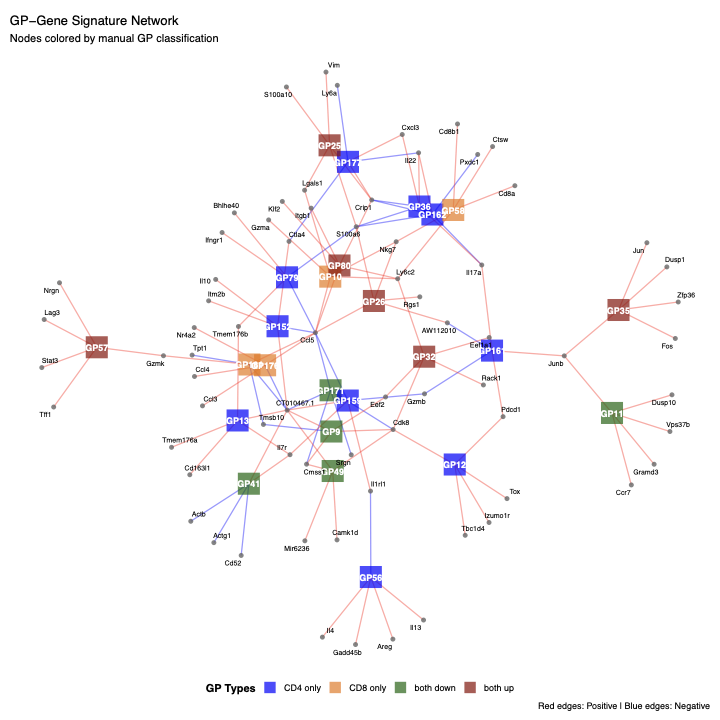

Fig. 3d. GP-gene signature network in which each GP is linked to its 5 most regulated marker genes (per-GP-normalized gene scores); edges are colored by the score sign (red, positive; blue, negative).

(3e) TF-GP network

# ============================================================
# 3c: Bipartite TF-GP network
# ============================================================
mm <- org.Mm.eg.db::org.Mm.eg.db
go2eg <- as.list(org.Mm.eg.db::org.Mm.egGO2ALLEGS)
tf_symbols <- AnnotationDbi::select(mm, keys = unique(unlist(go2eg)), columns = "SYMBOL", keytype = "ENTREZID")
tf <- c(
  sort(tf_symbols$SYMBOL[tf_symbols$ENTREZID %in% unique(go2eg[["GO:0003700"]])]),
  "Tox", "Tox2", "Tox3", "Tox4"
) %>% sort() %>% unique()

F_sub_tf <- F_pm_filtered_norm[, GPs_of_interest, drop = FALSE]
tf_gp_threshold <- 0.25
tf_in_F <- intersect(tf, rownames(F_sub_tf))
tf_max_score <- apply(F_sub_tf[tf_in_F, , drop = FALSE], 1, max, na.rm = TRUE)
selected_tfs <- sort(names(tf_max_score)[tf_max_score > tf_gp_threshold])

# Top-to-bottom group order in the network: both-up -> CD8-only -> both-down -> CD4-only
gp_color_group_order <- c("darkred", "darkorange2", "darkgreen", "blue")

tf_network_plot <- plot_tf_gp_network_v2(
  F = F_sub_tf,
  selected_tfs = selected_tfs,
  tf_gp_threshold = tf_gp_threshold,
  top_genes_per_gp = 5,
  gp_colors = highlight_colors,
  gp_group_order = gp_color_group_order,
  optimize_layout = TRUE,
  barycenter_iter = 12,
  gp_spacing = 1.5,
  node_size_tf = 6,
  node_size_gp = 5,
  label_size_tf = 4.5,
  label_size_gp = 4,
  label_size_gene = 3.4
)
plot_height_tf <- min(60, max(12, length(selected_tfs) * 0.35, length(GPs_of_interest) * 1.5 * 0.55 + 2))
ggsave(filename = paste0(figure_path, "3e.pdf"), plot = tf_network_plot, width = 18, height = plot_height_tf, limitsize = FALSE)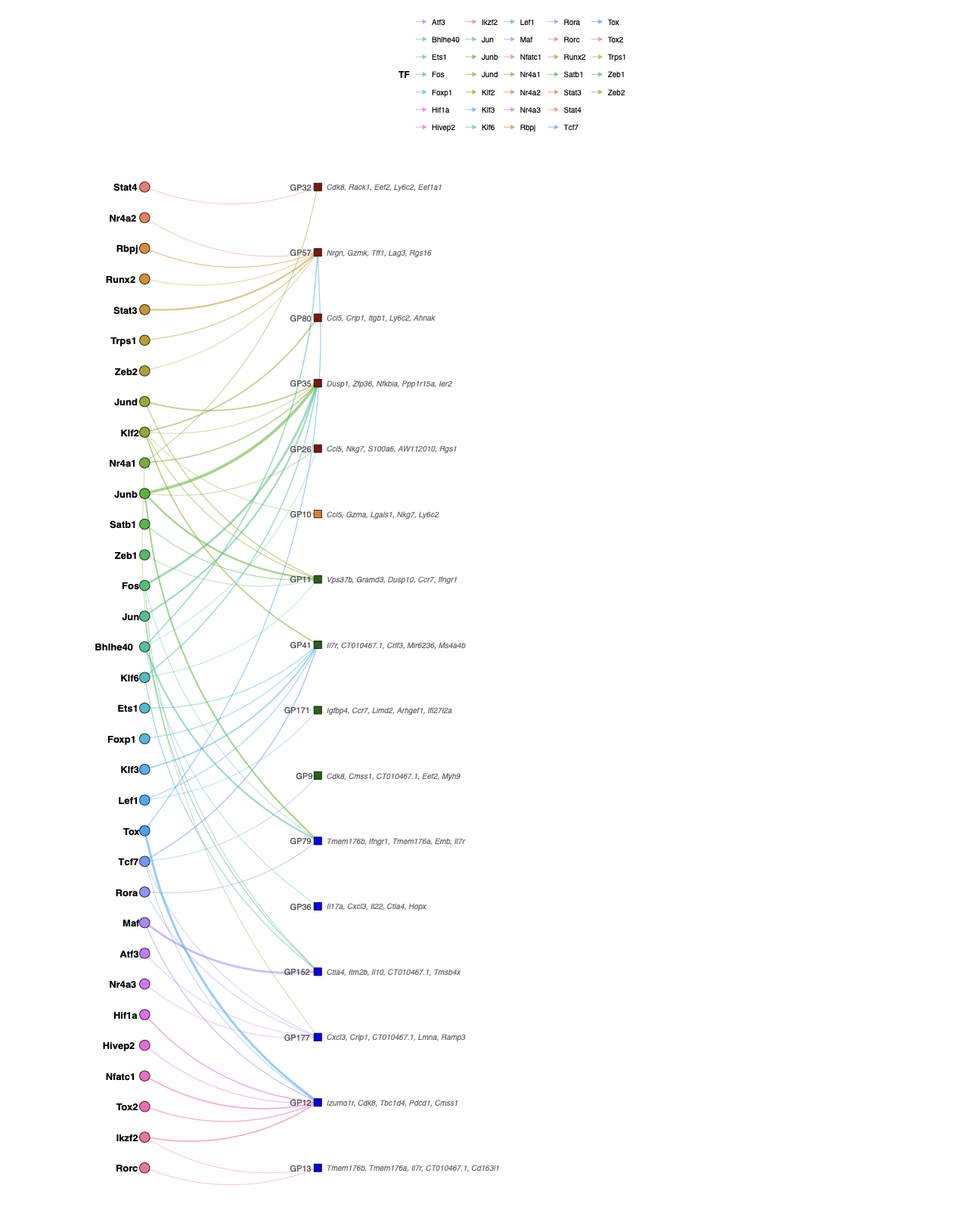

Fig. 3e. Bipartite transcription factor (TF)-GP network: TFs (GO:0003700 DNA-binding TFs plus the Tox family) with a normalized score exceeding 0.25 in any curated GP are connected to those GPs by directed edges (width proportional to the normalized score, color identifying the TF); the top 5 positively regulated genes per GP are listed beside each GP node.

(3f) Log2FC heatmap across conditions

# ============================================================
# 3d: log2FC heatmap of activated CD4+CD8 cells across conditions,
#     relative to the per-GP mean across all CD4/CD8 cells
# ============================================================
act_keep <- seurat_meta_filtered$annotation_level1 %in% c("CD4", "CD8") & seurat_meta_filtered$annotation_level2_group == "activated"
meta_act <- seurat_meta_filtered[act_keep, ]
L_act <- L_subset[act_keep, , drop = FALSE]

min_cells_cond <- 50
cd_lin <- table(meta_act$condition_detailed_simplified, meta_act$annotation_level1)
cond_keep <- rownames(cd_lin)[cd_lin[, "CD4"] >= min_cells_cond & cd_lin[, "CD8"] >= min_cells_cond]

cd_br <- table(meta_act$condition_detailed_simplified, meta_act$condition_broad)
cd_to_broad <- setNames(colnames(cd_br)[apply(cd_br, 1, which.max)], rownames(cd_br))[cond_keep]

# Column order: `healthy` broad first (with `baseline` as its first condition)
broad_rank <- ifelse(cd_to_broad == "healthy", 0L, 1L)
within_broad_rank <- ifelse(cd_to_broad == "healthy" & cond_keep == "baseline", 0L, 1L)
col_order_cond <- order(broad_rank, cd_to_broad, within_broad_rank, cond_keep)
cond_keep <- cond_keep[col_order_cond]
cd_to_broad <- cd_to_broad[cond_keep]

mean_mat_cond <- vapply(cond_keep, function(cond) colMeans(L_act[meta_act$condition_detailed_simplified == cond, , drop = FALSE]), numeric(ncol(L_act)))
mean_mat_cond <- mean_mat_cond[gp_row_order, , drop = FALSE]
broad_levels <- unique(cd_to_broad)
col_anno_cond <- data.frame(condition_broad = factor(cd_to_broad, levels = broad_levels), row.names = colnames(mean_mat_cond))
row_label_cols <- group_colors[gp_to_group[gp_row_order]]

pc_lfc <- 1e-10
cap_lfc <- 2
cd4cd8_idx <- seurat_meta_filtered$annotation_level1 %in% c("CD4", "CD8")
L_cd4cd8 <- L_subset[cd4cd8_idx, , drop = FALSE]
mu_lfc_mean <- colMeans(L_cd4cd8, na.rm = TRUE)[rownames(mean_mat_cond)]
lfc_mat_mean <- log2((mean_mat_cond + pc_lfc) / (mu_lfc_mean + pc_lfc))
lfc_mat_mean <- pmax(pmin(lfc_mat_mean, cap_lfc), -cap_lfc)

ph_cond_lfc_mean <- pheatmap(
  lfc_mat_mean, cluster_rows = FALSE, cluster_cols = FALSE,
  color = colorRampPalette(c("#7A0177", "black", "#FFD700"))(101),
  breaks = seq(-cap_lfc, cap_lfc, length.out = 102),
  annotation_col = col_anno_cond,
  gaps_row = head(cumsum(lengths(gp_groups)), -1),
  gaps_col = head(cumsum(rle(as.character(cd_to_broad))$lengths), -1),
  main = "log2FC vs per-GP MEAN across all CD4/CD8 (activated CD4+CD8 by condition_detailed_simplified)",
  silent = TRUE
)
row_idx_lfc_m <- which(ph_cond_lfc_mean$gtable$layout$name == "row_names")
ph_cond_lfc_mean$gtable$grobs[[row_idx_lfc_m]]$gp$col <- row_label_cols

pdf(paste0(figure_path, "3f.pdf"), width = max(8, 0.18 * ncol(lfc_mat_mean) + 4), height = 6)
grid::grid.draw(ph_cond_lfc_mean$gtable)
invisible(dev.off())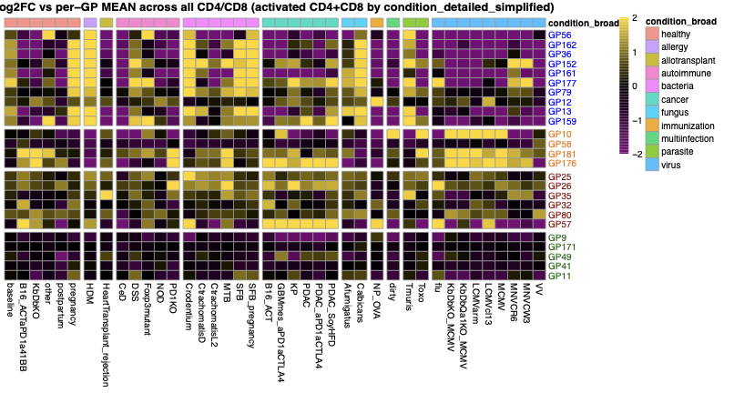

Fig. 3f. Heatmap of log2 fold-change in mean GP loading across experimental conditions for activated CD4 and CD8 cells, computed relative to each GP’s mean loading across all CD4/CD8 cells (resting and activated, all conditions) and capped at +-2, with a small pseudocount (1e-10) added to stabilize computation; columns are conditions with >=50 activated CD4 and >=50 activated CD8 cells, grouped and annotated by broad condition category, with color from purple (low) through black (no change) to gold (high).

(3g) Mean loading by sub-lineage

# ============================================================
# 3e: Mean GP loading per Level-2 sub-lineage (built before 3d since 3d
#     reuses gp_row_order/group_colors computed here)
# ============================================================
keep_cells <- seurat_meta_filtered$annotation_level1 %in% lineages
meta_sub <- seurat_meta_filtered[keep_cells, ]
L_keep <- L_subset[keep_cells, , drop = FALSE]

l2_counts <- table(meta_sub$annotation_level2)
l2_keep <- names(l2_counts)[l2_counts >= 50]
# Drop the "P" cluster and any "w..." clusters (wM, wW, etc.) across all lineages
l2_stripped <- sub("^[^._]+[._]", "", l2_keep)
exclude_l2 <- l2_stripped == "P" | grepl("^w", l2_stripped, ignore.case = TRUE) | grepl("[._]w", l2_keep, ignore.case = TRUE)
l2_keep <- l2_keep[!exclude_l2]

mean_mat <- vapply(l2_keep, function(l2) colMeans(L_keep[meta_sub$annotation_level2 == l2, , drop = FALSE]), numeric(ncol(L_keep)))
l2_to_l1 <- vapply(l2_keep, function(l2) as.character(meta_sub$annotation_level1[meta_sub$annotation_level2 == l2][1]), character(1))
col_order <- order(match(l2_to_l1, lineages), l2_keep)
mean_mat <- mean_mat[gp_row_order, col_order]
l2_to_l1 <- l2_to_l1[col_order]

immgen_cols <- ZemmourLib::immgent_colors
col_anno <- data.frame(Lineage = factor(l2_to_l1, levels = lineages), row.names = colnames(mean_mat))
anno_colors_mean <- list(Lineage = immgen_cols$level1[lineages])
row_label_cols <- group_colors[gp_to_group[gp_row_order]]
col_label_cols <- immgen_cols$level2[colnames(mean_mat)]
col_label_cols[is.na(col_label_cols)] <- "black"

ph <- pheatmap(
  mean_mat, cluster_rows = FALSE, cluster_cols = FALSE,
  color = colorRampPalette(c("white", "red"))(200),
  annotation_col = col_anno, annotation_colors = anno_colors_mean,
  gaps_row = head(cumsum(lengths(gp_groups)), -1),
  gaps_col = head(cumsum(rle(l2_to_l1)$lengths), -1),
  main = "Average loading of Figure 3 GPs per Level-2 sub-lineage",
  silent = TRUE
)
row_idx <- which(ph$gtable$layout$name == "row_names")
col_idx <- which(ph$gtable$layout$name == "col_names")
ph$gtable$grobs[[row_idx]]$gp$col <- row_label_cols
ph$gtable$grobs[[col_idx]]$gp$col <- col_label_cols

pdf(paste0(figure_path, "3g.pdf"), width = 11, height = 5.5)
grid::grid.draw(ph$gtable)
invisible(dev.off())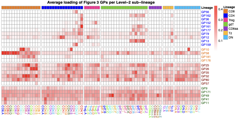

Fig. 3g. Heatmap of mean GP loading per Level-2 sub-lineage across the seven T-cell lineages (CD8, CD4, Treg, gdT, CD8aa, Tz, DN; sub-types with >=50 cells), with the top bar denoting parent lineage and color from white (low) to red (high).

Session information

sessionInfo()

R version 4.5.1 (2025-06-13)
Platform: aarch64-apple-darwin20
Running under: macOS Sequoia 15.6.1

Matrix products: default
BLAS:   /System/Library/Frameworks/Accelerate.framework/Versions/A/Frameworks/vecLib.framework/Versions/A/libBLAS.dylib 
LAPACK: /Library/Frameworks/R.framework/Versions/4.5-arm64/Resources/lib/libRlapack.dylib;  LAPACK version 3.12.1

locale:
[1] en_CA/en_CA/en_CA/C/en_CA/en_CA

time zone: Asia/Tokyo
tzcode source: internal

attached base packages:
[1] stats     graphics  grDevices utils     datasets  methods   base     

loaded via a namespace (and not attached):
 [1] vctrs_0.7.3     cli_3.6.6       knitr_1.50      rlang_1.2.0    
 [5] xfun_0.55       stringi_1.8.7   otel_0.2.0      promises_1.5.0 
 [9] jsonlite_2.0.0  workflowr_1.7.2 glue_1.8.1      rprojroot_2.1.1
[13] git2r_0.36.2    htmltools_0.5.9 httpuv_1.6.16   sass_0.4.10    
[17] rmarkdown_2.30  evaluate_1.0.5  jquerylib_0.1.4 tibble_3.3.0   
[21] fastmap_1.2.0   yaml_2.3.12     lifecycle_1.0.5 stringr_1.6.0  
[25] compiler_4.5.1  fs_1.6.6        Rcpp_1.1.1-1.1  pkgconfig_2.0.3
[29] later_1.4.4     digest_0.6.39   R6_2.6.1        pillar_1.11.1  
[33] magrittr_2.0.5  bslib_0.9.0     tools_4.5.1     cachem_1.1.0