Figure S1: GP reproducibility across IGTs
Ziang Zhang
Last updated: 2026-07-02
Checks: 5 1
Knit directory:
immgenT-GP-analysis/analysis/
This reproducible R Markdown analysis was created with workflowr (version 1.7.2). The Checks tab describes the reproducibility checks that were applied when the results were created. The Past versions tab lists the development history.
Great job! The global environment was empty. Objects defined in the global environment can affect the analysis in your R Markdown file in unknown ways. For reproduciblity it’s best to always run the code in an empty environment.
The command set.seed(1) was run prior to running the
code in the R Markdown file. Setting a seed ensures that any results
that rely on randomness, e.g. subsampling or permutations, are
reproducible.
Great job! Recording the operating system, R version, and package versions is critical for reproducibility.
Nice! There were no cached chunks for this analysis, so you can be confident that you successfully produced the results during this run.
Great job! Using relative paths to the files within your workflowr project makes it easier to run your code on other machines.
Tracking code development and connecting the code version to the
results is critical for reproducibility. To start using Git, open the
Terminal and type git init in your project directory.
This project is not being versioned with Git. To obtain the full
reproducibility benefits of using workflowr, please see
?wflow_start.
All panels are produced by script-refactor/FigureS1.R.
The code below is shown for reference (not re-executed on this page);
the images are its pre-rendered output. Panels A/B reuse a cached
per-IGT cosine-similarity score matrix
(data/igt_specific_cosine_scores.csv); see
code-refactor/pipeline/05_igt_validation.R for how that
matrix itself is produced (a much heavier, cluster-scale
computation).
Setup
# Figure S1. GP reproducibility across IGTs.
#
# Panels produced (see figures/final-selected/bits/Figure S1/FigureS1_caption.md
# for the full caption text):
#   S1A  Cumulative number of GPs validated (cosine >= threshold, thresholds
#        0.2-0.8) as IGTs are added one at a time, in IGT index order.
#   S1B  Number of GPs validated by at least X IGTs, vs X (log-log), for the
#        same thresholds.
#   S1C  Between-IGT variability: each GP's mean-of-per-IGT-mean-loading (x)
#        vs. variance-of-per-IGT-mean-loading (y), spleen-standard subset.
#   S1D  Heatmap of per-IGT mean loading for the 10 highest-variance GPs from
#        S1C (IGTs with >= 500 spleen-standard cells only).
#
# Source: S1A/S1B ported from script/Figure_Saturation.R; S1C/S1D from
# script/Figure_batch.R (panels a/b only -- that script's `plot_gp_loading()`
# helper is defined but never called for a saved output, so it's dropped).
#
# S1A/S1B reuse the per-IGT cosine-matching score matrix
# (data/igt_specific_cosine_scores.csv) rather than recomputing it here --
# recomputing requires Hungarian-matching each of the ~80 per-IGT
# refactorizations in data/igt_specific/*.qs against the full model, which is
# the job of code-refactor/pipeline/05_igt_validation.R (run once upstream).

library(dplyr)
library(tidyr)
library(ggplot2)
library(pheatmap)

data_path <- "data/"
figure_path <- "figure-refactor/Figure S1/"
gp_label <- function(x) sub("^K(\\d+)$", "GP\\1", x)
Panels A and B both use the cached per-IGT cosine score matrix:
# ============================================================
# S1A/S1B: load the cached per-IGT cosine score matrix
# (GPs x IGTs; produced by code-refactor/pipeline/05_igt_validation.R)
# ============================================================
score_mat <- as.matrix(read.csv(paste0(data_path, "igt_specific_cosine_scores.csv"), row.names = 1, check.names = FALSE))
(A) Cumulative GPs validated as IGTs are added
# ============================================================
# S1A: cumulative number of GPs validated as IGTs are added, in IGT-index order
# ============================================================
igt_idx <- as.integer(gsub("^IGT", "", colnames(score_mat)))
o <- order(igt_idx)
score_mat_ord <- score_mat[, o, drop = FALSE]

cum_validated_counts <- function(score_mat_ord, threshold) {
  validated <- score_mat_ord >= threshold
  ever_validated <- t(apply(validated, 1, cummax)) # 200 x nIGT logical
  colSums(ever_validated)
}
plot_df_a <- lapply(thresholds, function(t) {
  y <- cum_validated_counts(score_mat_ord, t)
  data.frame(n_IGTs_included = seq_along(y), validated_GPs = y, threshold = factor(t))
}) %>% bind_rows()

p_S1A <- ggplot(plot_df_a, aes(x = n_IGTs_included, y = validated_GPs, color = threshold)) +
  geom_line(linewidth = 1) +
  geom_point(size = 1) +
  labs(x = "Number of IGTs included (in IGT index order)", y = "Number of validated GPs (cumulative union)", color = "Threshold") +
  theme_minimal() +
  scale_color_brewer(palette = "Set1") +
  scale_x_continuous(breaks = seq(0, ncol(score_mat_ord), by = 5)) +
  scale_y_continuous(breaks = seq(0, max(plot_df_a$validated_GPs), by = 20))
ggsave(paste0(figure_path, "S1A.pdf"), plot = p_S1A, width = 6, height = 4)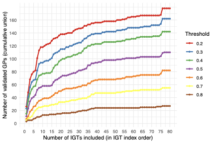
Fig. S1A. GPs were tested for reproducibility in individual datasets (IGTs): for each IGT a dataset-specific EBMF factorization was computed and its factors were matched to the global GPs by Hungarian assignment on the cosine similarity of gene-score vectors (restricted to shared genes, with columns scaled), and a GP is counted as “validated” in an IGT when this cosine similarity reaches a given threshold. Adding IGTs one at a time in index order, the curves show the cumulative number of GPs (of 200) validated in at least one IGT included so far, for cosine thresholds of 0.2-0.8.
(B) GPs validated by at least X IGTs
# ============================================================
# S1B: number of GPs validated by at least X IGTs, vs X (log-log)
# ============================================================
thresholds <- seq(0.2, 0.8, by = 0.1)
X_grid <- 1:50
plot_df_b <- tidyr::crossing(threshold = thresholds, X = X_grid) %>%
  mutate(n_GP = purrr::map2_int(threshold, X, \(t, x) {
    rowSums(score_mat >= t, na.rm = TRUE) |> (\(v) sum(v >= x))()
  }))

p_S1B <- ggplot(plot_df_b, aes(x = X, y = n_GP, group = factor(threshold))) +
  geom_line() +
  geom_point(size = 1) +
  scale_y_log10() +
  scale_x_log10() +
  labs(x = "X (validated by at least X IGTs)", y = "Number of GPs", color = "Threshold") +
  aes(color = factor(threshold)) +
  theme_minimal() +
  scale_color_brewer(palette = "Set1")
ggsave(paste0(figure_path, "S1B.pdf"), plot = p_S1B, width = 6, height = 4)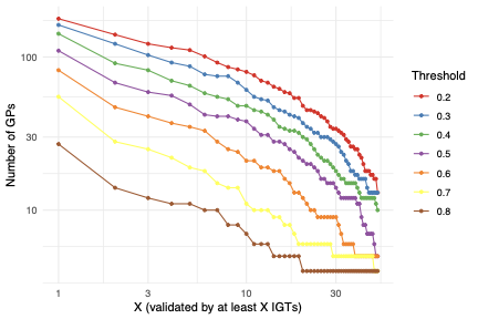
Fig. S1B. Using the same per-IGT cosine matching, the number of GPs validated by at least X IGTs as a function of X (both axes log-scaled), for thresholds of 0.2-0.8.
(C) Between-IGT variability
# ============================================================
# Load data for S1C/S1D
# ============================================================
L_pm_filtered <- readRDS(paste0(data_path, "L_pm_filtered.rds"))
seurat_meta <- readRDS(paste0(data_path, "igt1_96_withtotalvi20260206_clean_ADTonly.Rds"))@meta.data
seurat_meta_filtered <- seurat_meta[rownames(L_pm_filtered), ]
seurat_meta_filtered_spleen <- seurat_meta_filtered %>% filter(spleen_standard == TRUE)
all_gps <- paste0("K", 1:200)
selected_igts <- names(table(seurat_meta_filtered_spleen$IGT))[table(seurat_meta_filtered_spleen$IGT) >= 500]
# ============================================================
# S1C: GP mean-of-IGT-mean-loading vs. variance-of-IGT-mean-loading (spleen)
# ============================================================
common_cells_c <- intersect(rownames(L_pm_filtered), rownames(seurat_meta_filtered_spleen))
L_sub_c <- L_pm_filtered[common_cells_c, ]
igt_vec_c <- seurat_meta_filtered_spleen[common_cells_c, "IGT"]
igt_levels_c <- unique(igt_vec_c)
igt_mat_c <- do.call(rbind, lapply(igt_levels_c, function(igt) colMeans(L_sub_c[igt_vec_c == igt, , drop = FALSE])))
gp_igt_var <- apply(igt_mat_c, 2, var)
gp_overall <- colMeans(igt_mat_c)
gp_stats <- data.frame(GP = colnames(L_sub_c), x = gp_overall, y = gp_igt_var) %>%
arrange(desc(y)) %>%
mutate(label = ifelse(row_number() <= 10, gp_label(as.character(GP)), ""))
p_S1C <- ggplot(gp_stats, aes(x = x, y = y, label = label)) +
geom_point(size = 1.5, alpha = 0.7, color = "steelblue") +
ggrepel::geom_text_repel(size = 3, box.padding = 0.4, max.overlaps = Inf, segment.color = "grey50") +
cowplot::theme_cowplot() +
labs(
title = "GP Mean of IGT Mean Loading vs. Between-IGT VAR",
x = "Mean of IGT Mean Loading",
y = "Variance of IGT Mean Loading"
)
ggsave(paste0(figure_path, "S1C.pdf"), plot = p_S1C, width = 6, height = 5, dpi = 300)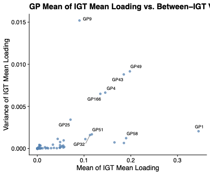
Fig. S1C. Between-IGT variability of GP loadings, computed on a standard spleen subset used for this purpose. Each GP’s mean loading is computed within every IGT; each point is a GP, plotting the mean across IGTs of these per-IGT mean loadings (x-axis) against their variance across IGTs (y-axis). The ten GPs with the highest between-IGT variance are labeled.
(D) Top-variance GP heatmap
# ============================================================
# S1D: heatmap of per-IGT mean loading for the top-10 variance GPs from S1C
#      (IGTs with >= 500 spleen-standard cells only)
# ============================================================
top10_var_gps <- names(sort(gp_igt_var, decreasing = TRUE))[1:10]

spleen_cells_act <- intersect(rownames(L_pm_filtered), rownames(seurat_meta_filtered_spleen))
igt_vec_act <- seurat_meta_filtered_spleen[spleen_cells_act, "IGT"]
igt_mean_mat_act <- do.call(rbind, lapply(selected_igts, function(igt) {
  cells_i <- spleen_cells_act[igt_vec_act == igt]
  colMeans(L_pm_filtered[cells_i, all_gps, drop = FALSE])
}))
rownames(igt_mean_mat_act) <- selected_igts

plot_mat <- t(igt_mean_mat_act[, top10_var_gps, drop = FALSE])
plot_mat[plot_mat < 0] <- 0
rownames(plot_mat) <- gp_label(rownames(plot_mat))

pdf(paste0(figure_path, "S1D.pdf"), width = 5, height = 5)
pheatmap(
  plot_mat,
  cluster_rows = TRUE,
  cluster_cols = FALSE,
  main = "Top 10 GPs by Variance of IGT Mean Loading",
  color = colorRampPalette(c("white", "red"))(100),
  border_color = "white",
  fontsize_row = 8,
  angle_col = 45
)
dev.off()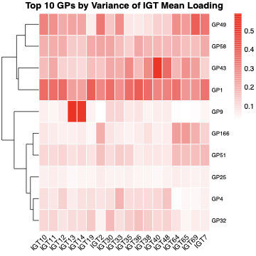
Fig. S1D. Heatmap of the per-IGT mean loading (same standard spleen subset, restricted to IGTs with >= 500 cells) for the ten GPs with the highest between-IGT variance from (C). Rows (GPs) are hierarchically clustered; color runs from white (low) to red (high mean loading).
sessionInfo()R version 4.5.1 (2025-06-13)
Platform: aarch64-apple-darwin20
Running under: macOS Sequoia 15.6.1
Matrix products: default
BLAS: /System/Library/Frameworks/Accelerate.framework/Versions/A/Frameworks/vecLib.framework/Versions/A/libBLAS.dylib
LAPACK: /Library/Frameworks/R.framework/Versions/4.5-arm64/Resources/lib/libRlapack.dylib; LAPACK version 3.12.1
locale:
[1] en_CA/en_CA/en_CA/C/en_CA/en_CA
time zone: Asia/Tokyo
tzcode source: internal
attached base packages:
[1] stats graphics grDevices utils datasets methods base
loaded via a namespace (and not attached):
[1] vctrs_0.7.3 cli_3.6.6 knitr_1.50 rlang_1.2.0
[5] xfun_0.55 stringi_1.8.7 otel_0.2.0 promises_1.5.0
[9] jsonlite_2.0.0 workflowr_1.7.2 glue_1.8.1 rprojroot_2.1.1
[13] git2r_0.36.2 htmltools_0.5.9 httpuv_1.6.16 sass_0.4.10
[17] rmarkdown_2.30 evaluate_1.0.5 jquerylib_0.1.4 tibble_3.3.0
[21] fastmap_1.2.0 yaml_2.3.12 lifecycle_1.0.5 stringr_1.6.0
[25] compiler_4.5.1 fs_1.6.6 Rcpp_1.1.1-1.1 pkgconfig_2.0.3
[29] later_1.4.4 digest_0.6.39 R6_2.6.1 pillar_1.11.1
[33] magrittr_2.0.5 bslib_0.9.0 tools_4.5.1 cachem_1.1.0