Figure 1: Overview of the 200 gene programs in immgenT
Ziang Zhang
Last updated: 2026-08-19
Checks: 7 0
Knit directory:
immgenT-GP-analysis/analysis/
This reproducible R Markdown analysis was created with workflowr (version 1.7.2). The Checks tab describes the reproducibility checks that were applied when the results were created. The Past versions tab lists the development history.
Great! Since the R Markdown file has been committed to the Git repository, you know the exact version of the code that produced these results.
Great job! The global environment was empty. Objects defined in the global environment can affect the analysis in your R Markdown file in unknown ways. For reproduciblity it’s best to always run the code in an empty environment.
The command set.seed(1) was run prior to running the
code in the R Markdown file. Setting a seed ensures that any results
that rely on randomness, e.g. subsampling or permutations, are
reproducible.
Great job! Recording the operating system, R version, and package versions is critical for reproducibility.
Nice! There were no cached chunks for this analysis, so you can be confident that you successfully produced the results during this run.
Great job! Using relative paths to the files within your workflowr project makes it easier to run your code on other machines.
Great! You are using Git for version control. Tracking code development and connecting the code version to the results is critical for reproducibility.
The results in this page were generated with repository version adc2327. See the Past versions tab to see a history of the changes made to the R Markdown and HTML files.
Note that you need to be careful to ensure that all relevant files for
the analysis have been committed to Git prior to generating the results
(you can use wflow_publish or
wflow_git_commit). workflowr only checks the R Markdown
file, but you know if there are other scripts or data files that it
depends on. Below is the status of the Git repository when the results
were generated:
Ignored files:
    Ignored:    .DS_Store
    Ignored:    .claude/
    Ignored:    analysis/.DS_Store
    Ignored:    analysis/.Rhistory
    Ignored:    analysis/assets/.DS_Store
    Ignored:    captions/
    Ignored:    code/.DS_Store
    Ignored:    code/other/topic_flashier_20250212.R
    Ignored:    code/other/topic_wrapper_20250215_alldata_backfit.sh
    Ignored:    data
    Ignored:    experiments/
    Ignored:    figures/.DS_Store
    Ignored:    figures/Previous/.DS_Store
    Ignored:    figures/Previous/bits/.DS_Store
    Ignored:    figures/Previous/bits/Figure 1/.DS_Store
    Ignored:    figures/Previous/bits/Figure 2/.DS_Store
    Ignored:    figures/Previous/bits/Figure 3/.DS_Store
    Ignored:    figures/Previous/bits/Figure 4/.DS_Store
    Ignored:    figures/Previous/bits/Figure 6/.DS_Store
    Ignored:    figures/Previous/bits/Figure 7/.DS_Store
    Ignored:    figures/Previous/bits/Figure S1/.DS_Store
    Ignored:    figures/Previous/bits/Figure S2/.DS_Store
    Ignored:    figures/Previous/bits/Figure S3/.DS_Store
    Ignored:    figures/Previous/bits/Figure S6/.DS_Store
    Ignored:    figures/Previous/bits/Figure S7/.DS_Store
    Ignored:    figures/final-selected/.DS_Store
    Ignored:    figures/final-selected/Figure 1/.DS_Store
    Ignored:    figures/final-selected/Figure 2/.DS_Store
    Ignored:    figures/final-selected/Figure 4/.DS_Store
    Ignored:    figures/final-selected/Figure S1/.DS_Store
    Ignored:    figures/final-selected/Figure S4/.DS_Store
    Ignored:    figures/templates_20260729/
    Ignored:    log/
    Ignored:    output/.DS_Store
    Ignored:    output/Figure2/
    Ignored:    output/Figure7b/7b_cell_metadata.csv.gz
    Ignored:    plan/
    Ignored:    tables/
    Ignored:    tmp/
Note that any generated files, e.g. HTML, png, CSS, etc., are not included in this status report because it is ok for generated content to have uncommitted changes.
These are the previous versions of the repository in which changes were
made to the R Markdown (analysis/Figure1.Rmd) and HTML
(docs/Figure1.html) files. If you’ve configured a remote
Git repository (see ?wflow_git_remote), click on the
hyperlinks in the table below to view the files as they were in that
past version.
| File | Version | Author | Date | Message |
|---|---|---|---|---|
| Rmd | adc2327 | Ziang Zhang | 2026-08-19 | Site prose: finish taking internal notes off the pages |
| html | 074dca1 | Ziang Zhang | 2026-08-05 | Build site: Extended Data tables reordered to six, internal notes off the pages |
| html | cbcec52 | Ziang Zhang | 2026-07-30 | Build site: Extended Data Figure naming |
| html | ac650a0 | Ziang Zhang | 2026-07-30 | Build site: Figure S5 (ex-S6a) and Figure S6 as a-f |
| html | ae21d37 | Ziang Zhang | 2026-07-28 | Build site: republish after the reorder commits |
| html | d538aa2 | Ziang Zhang | 2026-07-28 | Build site: reordered Figures 6 / S6 / S3 and the new Figure 7b page |
| html | 029b0ae | Ziang Zhang | 2026-07-28 | Build site. |
| Rmd | 0f5b5da | Ziang Zhang | 2026-07-28 | Align all figure captions with captions_20260728_final.docx |
| html | 3fc3789 | Ziang Zhang | 2026-07-27 | Republish all 24 pages |
| html | 1390a03 | Ziang Zhang | 2026-07-27 | Republish all 24 pages |
| html | adaef21 | Ziang Zhang | 2026-07-27 | Build site: panel fixes and PDF-derived assets |
| html | 5b19858 | Ziang Zhang | 2026-07-27 | Build site. |
| Rmd | ffe285c | Ziang Zhang | 2026-07-27 | Reorganize figures/ and untrack local-only exploration notes |
| Rmd | 91ee059 | Ziang Zhang | 2026-07-26 | Select each panel’s code block by name, not by line number |
| html | 91ee059 | Ziang Zhang | 2026-07-26 | Select each panel’s code block by name, not by line number |
| Rmd | c78e3cd | Ziang Zhang | 2026-07-16 | Fig 1D: publication version (highlighted GPs only, no legend) |
| html | c78e3cd | Ziang Zhang | 2026-07-16 | Fig 1D: publication version (highlighted GPs only, no legend) |
| Rmd | b197499 | Ziang Zhang | 2026-07-16 | Restructure main figures (renumber + split Figure 1) |
| html | b197499 | Ziang Zhang | 2026-07-16 | Restructure main figures (renumber + split Figure 1) |
| html | c70b79d | Ziang Zhang | 2026-07-15 | Make Fig 1C / GP-highlight figures square (20x20) |
| Rmd | c7dafe5 | Ziang Zhang | 2026-07-15 | Switch Figure 1C to GP-highlight gene-program network |
| html | c7dafe5 | Ziang Zhang | 2026-07-15 | Switch Figure 1C to GP-highlight gene-program network |
| Rmd | cac4f30 | Ziang Zhang | 2026-07-14 | Replace Figure 1C heatmap with gene-program network |
| html | cac4f30 | Ziang Zhang | 2026-07-14 | Replace Figure 1C heatmap with gene-program network |
| Rmd | c2b3360 | Ziang Zhang | 2026-07-13 | Use log-scale axes for Fig 1E/1F and add Fig S1E gene-vs-cell sparsity scatter |
| html | c2b3360 | Ziang Zhang | 2026-07-13 | Use log-scale axes for Fig 1E/1F and add Fig S1E gene-vs-cell sparsity scatter |
| html | 92021bf | Ziang Zhang | 2026-07-02 | Build site. |
| html | 827c89b | Ziang Zhang | 2026-07-02 | Build site. |
| Rmd | 8ac7f9f | Ziang Zhang | 2026-07-02 | Add data provenance notes to each script; remove conversational |
| Rmd | f9db962 | Ziang Zhang | 2026-07-02 | Simplify layout: drop old code/script folders, rename |
| html | c6e5086 | Ziang Zhang | 2026-07-02 | Build site. |
| html | 5a79883 | Ziang Zhang | 2026-07-02 | Build site. |
| Rmd | 2b0e445 | Ziang Zhang | 2026-07-02 | Fix GitHub source links to point at the new |
| html | cf1d0ac | Ziang Zhang | 2026-07-02 | Build site. |
| Rmd | 06b2461 | Ziang Zhang | 2026-07-02 | Initial commit: immgenT-GP-analysis |
| html | 06b2461 | Ziang Zhang | 2026-07-02 | Initial commit: immgenT-GP-analysis |
All panels except (B) are produced by script/Figure1.R.
The code below is shown for reference (not re-executed on this page,
since some steps such as the panel-D heatmap are slow); the images are
its pre-rendered output.
Setup
Data loading, shared across all panels below.
library(ggplot2)
library(dplyr)
library(scattermore)
library(ComplexHeatmap)
library(circlize)
library(tibble)
library(Matrix) # protein_mat_normalized_lognorm is a dgCMatrix; must be
                # attached (not just loaded) for `[` subsetting to dispatch

data_path <- "data/"
figure_path <- "figures/final-selected/Figure 1/"
source("code/R/volcano_helpers.R") # plot_gp_signature_volcano() for panel 1D

# ============================================================
# Load data
# ============================================================
flashier_snmf_summary <- readRDS(paste0(data_path, "flashier_snmf_summary.rds"))
L_pm_filtered <- readRDS(paste0(data_path, "L_pm_filtered.rds"))
F_pm_filtered <- readRDS(paste0(data_path, "F_pm_filtered.rds"))
seurat_meta <- readRDS(paste0(data_path, "igt1_96_withtotalvi20260206_clean_ADTonly.Rds"))@meta.data
seurat_meta_filtered <- seurat_meta[rownames(L_pm_filtered), ]
protein_mat_normalized_lognorm <- readRDS(paste0(data_path, "protein_mat_normalized_lognorm.rds"))
protein_mat_normalized_lognorm <- protein_mat_normalized_lognorm[rownames(L_pm_filtered), "CD44"]
mde_result <- readRDS(paste0(data_path, "umap_result.rds"))
colnames(mde_result) <- c("MDE_1", "MDE_2")
mde_result <- mde_result[rownames(L_pm_filtered), ]
df_mde <- as.data.frame(mde_result)
Panels C and D restrict to non-thymocyte cells:
# Drop thymocytes from all downstream cell-level visualizations.
non_thymo_cells <- seurat_meta_filtered$cellID[seurat_meta_filtered$annotation_level1 != "thymocyte"]
L_pm_filtered <- L_pm_filtered[non_thymo_cells, ]
seurat_meta_filtered <- seurat_meta_filtered[non_thymo_cells, ]
protein_mat_normalized_lognorm <- protein_mat_normalized_lognorm[non_thymo_cells]
(A) All-T MDE by lineage
# ============================================================
# 1A: Global MDE colored by major lineage, subsampled per lineage
# ============================================================
set.seed(1)
df_mde_a <- df_mde %>% tibble::rownames_to_column("cellID")
plot_df <- df_mde_a %>%
  inner_join(seurat_meta_filtered %>% select(cellID, annotation_level1), by = "cellID") %>%
  filter(annotation_level1 != "thymocyte")
max_total <- 1000000
min_per_group <- 300
cap_per_group <- 20000
group_sizes <- plot_df %>% count(annotation_level1, name = "n")
G <- nrow(group_sizes)
base_per_group <- ceiling(max_total / max(G, 1))
sample_plan <- group_sizes %>% mutate(n_take = pmin(n, pmax(min_per_group, pmin(cap_per_group, base_per_group))))
plot_df_sub <- plot_df %>%
  group_by(annotation_level1) %>%
  group_modify(~ dplyr::slice_sample(.x, n = sample_plan$n_take[sample_plan$annotation_level1 == .y$annotation_level1])) %>%
  ungroup()

p_1A <- ggplot(plot_df_sub, aes(x = MDE_1, y = MDE_2)) +
  scattermore::geom_scattermore(aes(color = annotation_level1), pointsize = 1.2) +
  scale_color_manual(values = ZemmourLib::immgent_colors$level1) +
  coord_equal() +
  theme_classic() +
  labs(title = "MDE: Annotation Level 1", x = "MDE 1", y = "MDE 2", color = "Cell Type") +
  theme(legend.text = element_text(size = 10), legend.key.size = unit(1.5, "lines")) +
  guides(color = guide_legend(override.aes = list(size = 4)))
ggsave(filename = paste0(figure_path, "1A.pdf"), plot = p_1A, width = 5, height = 5)

# 1B: hand-finished Illustrator schematic -- not code-generated, no output here.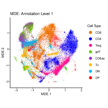
Fig. 1A. Minimum distortion embedding (MDE) of all mature T cells profiled in immgenT (the “all-T MDE”, i.e. all non-thymocyte cells), colored by T cell lineage: CD4, conventional CD4+ T cells; CD8, conventional CD8αβ+ T cells; Treg, CD4+ Foxp3+ regulatory T cells; CD8aa, CD8αα αβ T cells; gdT, γδ T cells; Tz, Zbtb16+ αβ T cells; DN, CD4-CD8αβ- αβ T cells; DP, CD4+CD8αβ+ αβ T cells. Cells are subsampled per lineage for visualization.
(B) GP-representation schematic
This panel is a hand-drawn schematic, not generated from code.
Fig. 1B. Schematic of the gene-program (GP) representation of T cell gene-expression profiles. Each cell is represented by a combination of GP activities (loadings), and each GP captures coordinated up- or downregulation of a subset of genes. Gene programs were learned from gene expression by empirical Bayes matrix factorization (EBMF): X ≈ LFᵀ (cells × genes matrix ≈ cells × GPs matrix · GPs × genes matrix). See Methods: fitting EBMF using flashier.
(C) Gene-program network
# ============================================================
# 1C: gene-program network -- the 200 GPs linked by their shared top signature
# genes, with a selected set of GPs highlighted. Each highlighted GP's color runs
# along its edges to its top signature genes (which are labeled); non-highlighted
# GPs are grey. Formal version: no legend / no GP-index labels -- the color->GP
# mapping and interpretation are in the Fig 1C caption (analysis/Figure1.Rmd).
# ============================================================
suppressPackageStartupMessages({
  library(igraph); library(tidygraph); library(ggraph)
})
N_TOP   <- 5                                      # top up-genes taken per GP
SIG_THR <- 0.1                                    # min per-GP-normalized loading
GP_HIGHLIGHTS <- c(                               # GP -> highlight color
  GP68  = "pink2",  GP58  = "orange2", GP35  = "purple", GP171 = "blue",
  GP1   = "cyan2",  GP56  = "red2",    GP161 = "brown",  GP6   = "green2",
  GP7   = "green3", GP196 = "yellow3")
GP_COL   <- "darkgrey"                            # non-highlighted GP nodes
GENE_COL <- "#C7A76C"                             # gene nodes (tan)

Fn <- F_pm_filtered
colnames(Fn) <- paste0("GP", seq_len(ncol(Fn)))
Fn <- sweep(Fn, 2, apply(abs(Fn), 2, max), "/")   # per-GP (column) max-abs norm
GPs <- colnames(Fn)

# each GP -> its top up-regulated signature genes (normalized loading >= SIG_THR)
top_up <- lapply(GPs, function(j) { x <- Fn[, j]
  u <- names(sort(x, decreasing = TRUE))[1:N_TOP]; u[x[u] >= SIG_THR] })
names(top_up) <- GPs
edges <- do.call(rbind, lapply(GPs, function(g)
  if (length(top_up[[g]])) data.frame(GP = g, Gene = top_up[[g]]) else NULL))

# bipartite GP<->gene graph (every GP + all its top genes); plain FR layout
gi <- graph_from_data_frame(edges, directed = FALSE)
g  <- as_tbl_graph(gi, directed = FALSE)
gp_set <- unique(edges$GP)
set.seed(1)
lay <- layout_with_fr(gi)
colnames(lay) <- c("x", "y"); rownames(lay) <- V(gi)$name
nm <- g %>% activate(nodes) %>% pull(name)

# highlight selected GPs: color their node + edges, label the genes they connect to
hl <- intersect(names(GP_HIGHLIGHTS), gp_set)
hl_genes <- setdiff(unique(unlist(
  lapply(hl, function(gp) neighbors(gi, gp)$name))), gp_set)
g <- g %>% activate(nodes) %>% mutate(
  is_gp = name %in% gp_set,
  gp_fill = ifelse(is_gp & name %in% hl, unname(GP_HIGHLIGHTS[name]), GP_COL),
  label_gene = !is_gp & name %in% hl_genes,
  gene_lab = ifelse(label_gene, name, ""),
  gp_size = ifelse(is_gp, 3, NA_real_))
g <- g %>% activate(edges) %>% mutate(
  gp_end = ifelse(.N()$is_gp[from], .N()$name[from], .N()$name[to]),
  gp_edge_highlight = gp_end %in% hl,
  gp_edge_col = ifelse(gp_edge_highlight, unname(GP_HIGHLIGHTS[gp_end]), NA_character_))

p_1C <- ggraph(g, layout = "manual", x = lay[nm, "x"], y = lay[nm, "y"]) +
  geom_edge_link(aes(filter = !gp_edge_highlight), color = "black", alpha = 0.18, width = 0.32) +
  geom_edge_link(aes(filter = gp_edge_highlight, edge_colour = gp_edge_col), alpha = 0.95, width = 1.25) +
  geom_node_point(aes(filter = !is_gp), shape = 16, size = 1, color = GENE_COL, alpha = 0.75) +
  geom_node_point(aes(filter = is_gp, size = gp_size, fill = gp_fill),
                  shape = 21, color = "white", stroke = 0.5) +
  geom_node_text(aes(filter = label_gene, label = gene_lab), repel = TRUE,
                 color = "black", size = 5, fontface = "italic", max.overlaps = Inf) +
  scale_fill_identity() + scale_edge_colour_identity() +
  scale_size_identity() + scale_edge_width_identity() +
  scale_x_continuous(expand = expansion(mult = 0.08)) +
  scale_y_continuous(expand = expansion(mult = 0.08)) +
  theme_void(base_size = 12) +
  theme(plot.margin = margin(10, 10, 10, 10), legend.position = "none")
ggsave(filename = paste0(figure_path, "1C.pdf"), plot = p_1C, width = 20, height = 20)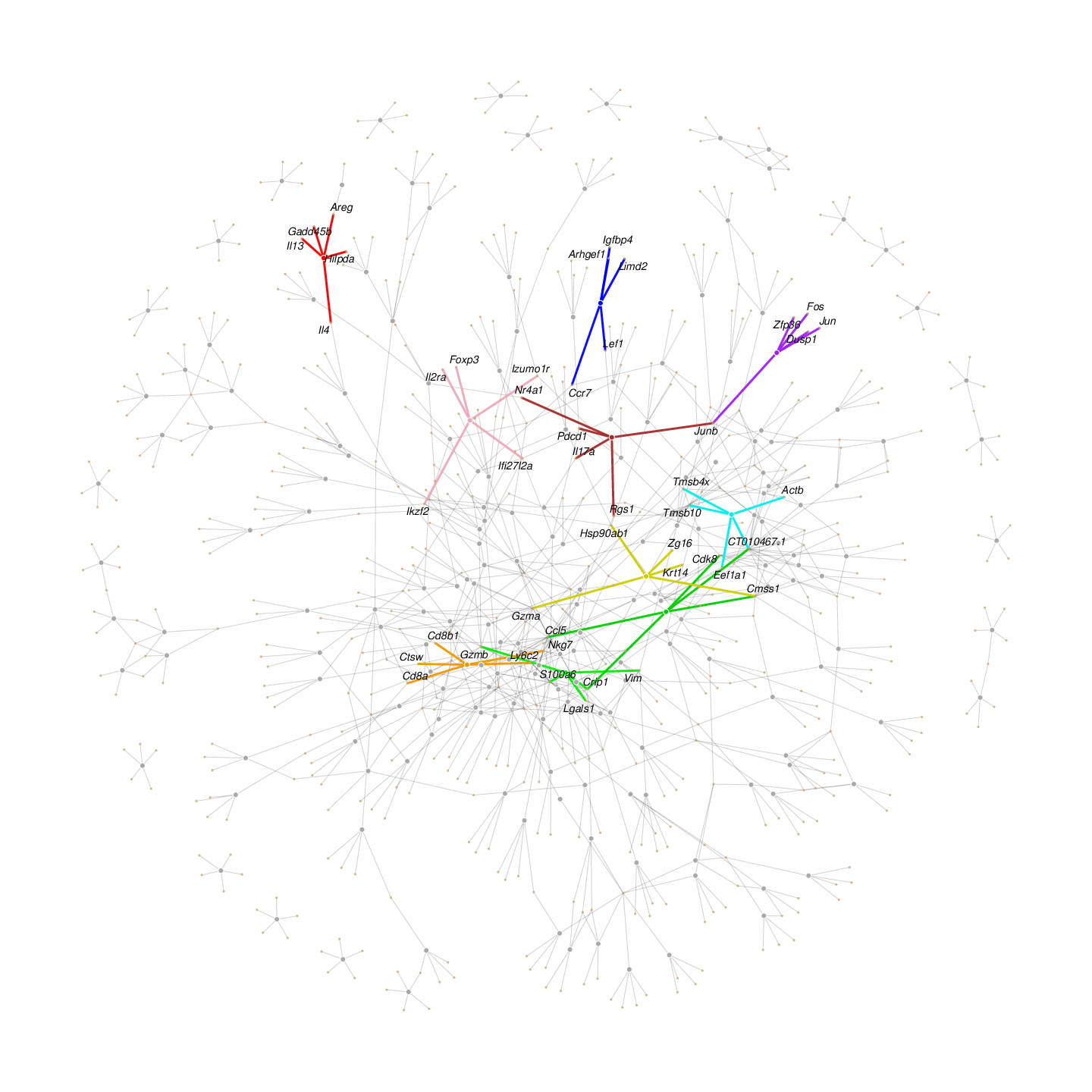
Fig. 1C. Gene-program (GP) network. A network summarizing the 200 GPs and the signature genes they share. Each GP’s gene scores are first normalized within the GP (divided by that GP’s maximum absolute gene score, so scores run 0–1), and every GP is joined to its top five up-regulated signature genes (largest positive normalized gene scores, ≥ 0.1). Grey nodes are GPs and tan nodes are genes; an edge joins a GP to each of its top signature genes, so a gene that appears among several GPs’ top genes links those GPs, and a force-directed layout places programs with overlapping signatures near one another. A selected set of GPs is highlighted, each in its own color carried along its edges to its (labeled) top signature genes: GP68 (pink), GP58 (orange), GP35 (purple), GP171 (blue), GP1 (cyan), GP56 (red), GP161 (dark red), GP6 (light green), GP7 (green), GP196 (yellow). This shows each highlighted program’s signature and how programs that share genes sit together — e.g. the Treg program GP68 (Foxp3, Il2ra, Izumo1r) and the CD8 program GP58 (Cd8a, Cd8b1) occupy distinct neighborhoods.
(D) GP loading heatmap
# ============================================================
# 1D: giant loading heatmap (200 GP loadings x a stratified cell sample; rows =
# cells by lineage x organ, columns = GPs clustered). The same GPs highlighted
# in the 1C network are marked here by a top color bar, a colored/bold column
# label, and a box around each GP column. See the Fig 1D caption (Figure1.Rmd).
# ============================================================
suppressPackageStartupMessages({ library(grid) })
GP_HIGHLIGHTS <- c(
  GP68 = "pink2",  GP58 = "orange2", GP35 = "purple", GP171 = "blue",
  GP1  = "cyan2",  GP56 = "red2",    GP161 = "brown", GP6  = "green2",
  GP7  = "green3", GP196 = "yellow3")

set.seed(6173)
MIN_CELLS <- 20; N_SAMPLE <- 80; TOP_ORGANS <- 5; K_ANCHOR <- 5
level1_order <- c("CD8", "CD4", "Treg", "gdT", "CD8aa", "Tz", "DN")
organs_all <- as.character(unique(seurat_meta_filtered$organ_simplified))
ln_match <- organs_all[grepl("^LN$|lymph", organs_all, ignore.case = TRUE)]
spleen_match <- organs_all[grepl("spleen", organs_all, ignore.case = TRUE)]
organ_order <- c(spleen_match, ln_match, sort(setdiff(organs_all, c(ln_match, spleen_match))))

top_organ_combos <- seurat_meta_filtered |>
  dplyr::filter(annotation_level1 %in% level1_order) |>
  dplyr::count(annotation_level1, organ_simplified) |>
  dplyr::group_by(annotation_level1) |>
  dplyr::slice_max(n, n = TOP_ORGANS, with_ties = FALSE) |>
  dplyr::ungroup() |> dplyr::select(annotation_level1, organ_simplified)
sampled_random <- seurat_meta_filtered |>
  dplyr::filter(annotation_level1 %in% level1_order) |>
  dplyr::inner_join(top_organ_combos, by = c("annotation_level1", "organ_simplified")) |>
  dplyr::group_by(annotation_level1, organ_simplified) |>
  dplyr::filter(dplyr::n() >= MIN_CELLS) |>
  dplyr::slice_sample(n = N_SAMPLE) |> dplyr::ungroup()
anchor_cellids <- apply(L_pm_filtered, 2, function(x)
  rownames(L_pm_filtered)[order(x, decreasing = TRUE)[seq_len(K_ANCHOR)]]) |> as.vector() |> unique()
anchor_meta <- seurat_meta_filtered |>
  dplyr::filter(cellID %in% anchor_cellids, annotation_level1 %in% level1_order) |>
  dplyr::inner_join(top_organ_combos, by = c("annotation_level1", "organ_simplified"))
all_meta <- dplyr::bind_rows(sampled_random, anchor_meta) |>
  dplyr::distinct(cellID, .keep_all = TRUE) |>
  dplyr::arrange(factor(annotation_level1, levels = level1_order),
                 factor(organ_simplified, levels = organ_order))

L_sampled <- L_pm_filtered[all_meta$cellID, ]
clip_val <- quantile(L_sampled, 0.99)
L_display <- pmin(L_sampled, clip_val)
colnames(L_display) <- gsub("^K", "GP", colnames(L_display))
col_fun <- colorRamp2(c(0, clip_val / 2, clip_val), c("white", "#4393c3", "#08306b"))
level1_present <- intersect(level1_order, as.character(unique(all_meta$annotation_level1)))
organ_present <- intersect(organ_order, as.character(unique(all_meta$organ_simplified)))
row_ann <- rowAnnotation(
  Cell_Type = factor(as.character(all_meta$annotation_level1), levels = level1_present),
  Organ = factor(as.character(all_meta$organ_simplified), levels = organ_present),
  col = list(Cell_Type = ZemmourLib::immgent_colors$level1[level1_present],
             Organ = ZemmourLib::immgent_colors$organ_simplified[organ_present]),
  annotation_name_gp = gpar(fontsize = 8),
  annotation_legend_param = list(Cell_Type = list(title = "Cell Type"), Organ = list(title = "Organ")))

gpn      <- colnames(L_display)
hl_val   <- ifelse(gpn %in% names(GP_HIGHLIGHTS), gpn, NA_character_)
lab_col  <- ifelse(gpn %in% names(GP_HIGHLIGHTS), GP_HIGHLIGHTS[gpn], "grey55")
lab_fs   <- ifelse(gpn %in% names(GP_HIGHLIGHTS), 9, 4)
lab_face <- ifelse(gpn %in% names(GP_HIGHLIGHTS), 2, 1)
# Publication version: only the highlighted GP columns keep an index label
# (background GP indices dropped), and the highlighted-GP legend is hidden -- the
# colour->GP mapping is given in the Fig 1D caption.
top_ann <- HeatmapAnnotation(
  `Highlighted GP` = hl_val, col = list(`Highlighted GP` = GP_HIGHLIGHTS),
  na_col = "white", simple_anno_size = unit(4, "mm"), annotation_name_gp = gpar(fontsize = 8),
  show_legend = FALSE)
ht_1D <- Heatmap(
  L_display, name = "Loading", col = col_fun, left_annotation = row_ann, top_annotation = top_ann,
  cluster_rows = FALSE, cluster_columns = TRUE,
  clustering_distance_columns = "euclidean", clustering_method_columns = "ward.D2",
  show_row_names = FALSE,
  column_labels = ifelse(gpn %in% names(GP_HIGHLIGHTS), gpn, ""),
  column_names_gp = gpar(col = lab_col, fontsize = lab_fs, fontface = lab_face),
  column_title = "Gene Programs (GPs)", column_title_gp = gpar(fontsize = 11, fontface = "bold"),
  use_raster = TRUE, raster_quality = 3, border = FALSE,
  heatmap_legend_param = list(title = "Loading", direction = "vertical"))
pdf(paste0(figure_path, "1D.pdf"), width = 15, height = 20, useDingbats = FALSE)
ht_drawn <- draw(ht_1D, merge_legend = TRUE)
co <- column_order(ht_drawn); disp <- colnames(L_display)[co]; n_col_ht <- length(co)
decorate_heatmap_body("Loading", {
  for (gp in names(GP_HIGHLIGHTS)) { j <- which(disp == gp)
    if (length(j)) grid.rect(x = (j - 0.5) / n_col_ht, y = 0.5, width = 1.4 / n_col_ht, height = 1,
                             gp = gpar(col = GP_HIGHLIGHTS[gp], fill = NA, lwd = 2.5)) } })
dev.off()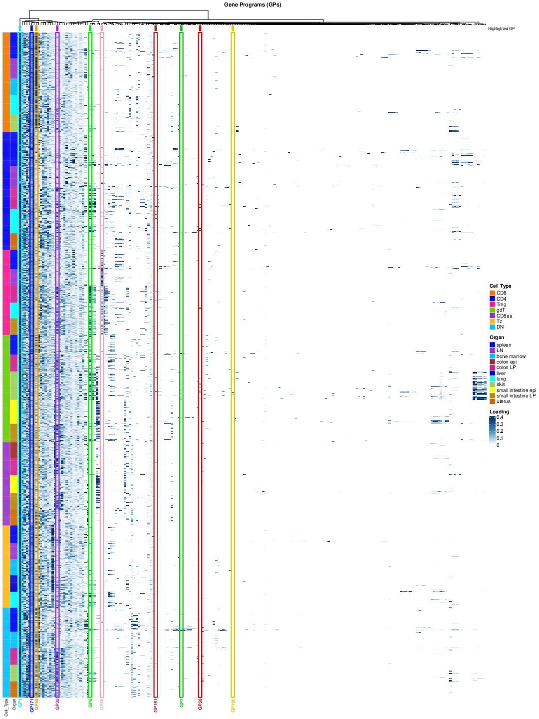
Fig. 1D. GP activity heatmap. Activity (loading) of all 200 GPs (columns) across T cells from different organs and lineages – a stratified sample of cells (rows), ordered by lineage then organ; the left strips annotate each cell’s cell type and organ, and GP columns are clustered by loading similarity. Loadings are clipped at the 99th percentile and run white → blue. Only the GPs highlighted in the (C) network are marked and labeled here (background GP column indices are omitted); each is shown in its matching color via a top color bar, a colored column label, and a box drawn around its column, so a program’s cross-cell loading pattern can be read alongside its position in the network. Colors: GP68 (pink), GP58 (orange), GP35 (purple), GP171 (blue), GP1 (cyan), GP56 (red), GP161 (dark red), GP6 (light green), GP7 (green), GP196 (yellow).
sessionInfo()R version 4.5.1 (2025-06-13)
Platform: aarch64-apple-darwin20
Running under: macOS Sequoia 15.6.1
Matrix products: default
BLAS: /System/Library/Frameworks/Accelerate.framework/Versions/A/Frameworks/vecLib.framework/Versions/A/libBLAS.dylib
LAPACK: /Library/Frameworks/R.framework/Versions/4.5-arm64/Resources/lib/libRlapack.dylib; LAPACK version 3.12.1
locale:
[1] en_CA/en_CA/en_CA/C/en_CA/en_CA
time zone: America/Chicago
tzcode source: internal
attached base packages:
[1] stats graphics grDevices utils datasets methods base
loaded via a namespace (and not attached):
[1] vctrs_0.7.3 cli_3.6.6 knitr_1.50 rlang_1.2.0
[5] xfun_0.55 stringi_1.8.7 otel_0.2.0 promises_1.5.0
[9] jsonlite_2.0.0 workflowr_1.7.2 glue_1.8.1 rprojroot_2.1.1
[13] git2r_0.36.2 htmltools_0.5.9 httpuv_1.6.16 sass_0.4.10
[17] rmarkdown_2.30 evaluate_1.0.5 jquerylib_0.1.4 tibble_3.3.0
[21] fastmap_1.2.0 yaml_2.3.12 lifecycle_1.0.5 whisker_0.4.1
[25] stringr_1.6.0 compiler_4.5.1 fs_1.6.6 Rcpp_1.1.1-1.1
[29] pkgconfig_2.0.3 later_1.4.4 digest_0.6.39 R6_2.6.1
[33] pillar_1.11.1 magrittr_2.0.5 bslib_0.9.0 tools_4.5.1
[37] cachem_1.1.0