Figure 2: Active cells and genes in gene programs
Ziang Zhang
Last updated: 2026-07-26
Checks: 6 1
Knit directory:
immgenT-GP-analysis/analysis/
This reproducible R Markdown analysis was created with workflowr (version 1.7.2). The Checks tab describes the reproducibility checks that were applied when the results were created. The Past versions tab lists the development history.
The R Markdown file has unstaged changes. To know which version of
the R Markdown file created these results, you’ll want to first commit
it to the Git repo. If you’re still working on the analysis, you can
ignore this warning. When you’re finished, you can run
wflow_publish to commit the R Markdown file and build the
HTML.
Great job! The global environment was empty. Objects defined in the global environment can affect the analysis in your R Markdown file in unknown ways. For reproduciblity it’s best to always run the code in an empty environment.
The command set.seed(1) was run prior to running the
code in the R Markdown file. Setting a seed ensures that any results
that rely on randomness, e.g. subsampling or permutations, are
reproducible.
Great job! Recording the operating system, R version, and package versions is critical for reproducibility.
Nice! There were no cached chunks for this analysis, so you can be confident that you successfully produced the results during this run.
Great job! Using relative paths to the files within your workflowr project makes it easier to run your code on other machines.
Great! You are using Git for version control. Tracking code development and connecting the code version to the results is critical for reproducibility.
The results in this page were generated with repository version f7d90e7. See the Past versions tab to see a history of the changes made to the R Markdown and HTML files.
Note that you need to be careful to ensure that all relevant files for
the analysis have been committed to Git prior to generating the results
(you can use wflow_publish or
wflow_git_commit). workflowr only checks the R Markdown
file, but you know if there are other scripts or data files that it
depends on. Below is the status of the Git repository when the results
were generated:
Ignored files:
    Ignored:    .DS_Store
    Ignored:    analysis/.DS_Store
    Ignored:    analysis/.Rhistory
    Ignored:    analysis/assets/.DS_Store
    Ignored:    code/.DS_Store
    Ignored:    data
    Ignored:    experiments/.DS_Store
    Ignored:    figures/.DS_Store
    Ignored:    figures/final-selected/.DS_Store
    Ignored:    figures/final-selected/bits/.DS_Store
    Ignored:    figures/final-selected/bits/Figure 1/.DS_Store
    Ignored:    figures/final-selected/bits/Figure 2/.DS_Store
    Ignored:    figures/final-selected/bits/Figure 3/.DS_Store
    Ignored:    figures/final-selected/bits/Figure 4/.DS_Store
    Ignored:    figures/final-selected/bits/Figure 6/.DS_Store
    Ignored:    figures/final-selected/bits/Figure 7/.DS_Store
    Ignored:    figures/final-selected/bits/Figure S1/.DS_Store
    Ignored:    figures/final-selected/bits/Figure S2/.DS_Store
    Ignored:    figures/final-selected/bits/Figure S3/.DS_Store
    Ignored:    figures/final-selected/bits/Figure S6/.DS_Store
    Ignored:    figures/final-selected/bits/Figure S7/.DS_Store
    Ignored:    figures/generated/.DS_Store
    Ignored:    figures/generated/Figure 1/.DS_Store
    Ignored:    figures/generated/Figure 2/.DS_Store
    Ignored:    output/FigureS5/S5_cell_metadata.csv.gz
    Ignored:    tmp/

Untracked files:
    Untracked:  .claude/
    Untracked:  code/R/doc_code.R
    Untracked:  code/other/topic_flashier_20250212.R
    Untracked:  code/other/topic_wrapper_20250215_alldata_backfit.sh
    Untracked:  experiments/active_metric_comparison/
    Untracked:  experiments/figure6b_sparsity_ordered/
    Untracked:  experiments/gene_umap_gp_space/
    Untracked:  experiments/protein_threshold_gp_loading_diff/
    Untracked:  experiments/surface_protein_activation_scatter/
    Untracked:  figures/generated/Figure 1/1B.pdf
    Untracked:  figures/generated/Figure 3/3A.pdf
    Untracked:  figures/generated/Figure 3/3B.pdf
    Untracked:  figures/generated/Figure 3/3H.pdf
    Untracked:  figures/generated/Figure 3/3I.pdf
    Untracked:  figures/generated/Figure 3/3J.pdf
    Untracked:  figures/generated/Figure 3/3K.pdf
    Untracked:  figures/generated/Figure 3/3L.pdf
    Untracked:  figures/generated/Figure 3/3M.pdf
    Untracked:  figures/generated/Figure 5/
    Untracked:  figures/generated/Figure 6/6a.pdf
    Untracked:  figures/generated/Figure 7/
    Untracked:  log/2026-07-13-surface-protein-activation-scatter.md
    Untracked:  log/2026-07-15-protein-threshold-gp-loading-diff-tables.md
    Untracked:  plan/2026-07-13-active-cell-gene-metrics-exploration.md
    Untracked:  plan/2026-07-13-surface-protein-activation-scatter.md
    Untracked:  plan/2026-07-13_figure6b_triangular_order_plan.md
    Untracked:  plan/2026-07-13_figure6b_wide_gp_columns_formal_plan.md
    Untracked:  plan/2026-07-14_figure6b_heatmap_typography_plan.md
    Untracked:  plan/2026-07-15-protein-threshold-gp-loading-diff-tables.md
    Untracked:  tables/

Unstaged changes:
    Modified:   analysis/Figure1.Rmd
    Modified:   analysis/Figure2.Rmd
    Modified:   analysis/Figure3.Rmd
    Modified:   analysis/Figure4.Rmd
    Modified:   analysis/Figure5.Rmd
    Modified:   analysis/Figure6.Rmd
    Modified:   analysis/FigureS1.Rmd
    Modified:   analysis/FigureS2.Rmd
    Modified:   analysis/FigureS3.Rmd
    Modified:   analysis/FigureS4.Rmd
    Modified:   analysis/FigureS6.Rmd
    Modified:   analysis/Methods_FlashierFit.Rmd
    Modified:   figures/generated/Figure 1/1A.pdf
    Modified:   figures/generated/Figure 1/1C.pdf
    Modified:   figures/generated/Figure 1/1D.pdf
    Deleted:    figures/generated/Figure 1/1E.pdf
    Deleted:    figures/generated/Figure 1/1F.pdf
    Deleted:    figures/generated/Figure 1/1G.pdf
    Deleted:    figures/generated/Figure 1/1H.pdf
    Deleted:    figures/generated/Figure 1/1I.pdf
    Modified:   figures/generated/Figure 2/2A.pdf
    Modified:   figures/generated/Figure 2/2B.pdf
    Modified:   figures/generated/Figure 2/2C.pdf
    Modified:   figures/generated/Figure 2/2D.pdf
    Modified:   figures/generated/Figure 2/2E.pdf
    Deleted:    figures/generated/Figure 2/2G.pdf
    Deleted:    figures/generated/Figure 2/2H.pdf
    Deleted:    figures/generated/Figure 2/2I.pdf
    Deleted:    figures/generated/Figure 2/2J.pdf
    Deleted:    figures/generated/Figure 2/2K.pdf
    Deleted:    figures/generated/Figure 2/2L.pdf
    Deleted:    figures/generated/Figure 2/2M.pdf
    Modified:   figures/generated/Figure 3/3c.pdf
    Modified:   figures/generated/Figure 3/3d.pdf
    Modified:   figures/generated/Figure 3/3e.pdf
    Modified:   figures/generated/Figure 3/3f.pdf
    Modified:   figures/generated/Figure 3/3g.pdf
    Modified:   figures/generated/Figure S1/S1A.pdf
    Modified:   figures/generated/Figure S1/S1B.pdf
    Modified:   figures/generated/Figure S1/S1C.pdf
    Modified:   figures/generated/Figure S1/S1D.pdf
    Modified:   figures/generated/Figure S1/S1E.pdf
    Modified:   figures/generated/Figure S3/s3c.pdf
    Modified:   figures/generated/Figure S3/s3d.pdf
    Modified:   figures/generated/Figure S3/s3e.pdf
    Modified:   figures/generated/Figure S3/s3f.pdf
    Modified:   figures/generated/Figure S3/s3g.pdf
    Modified:   figures/generated/Figure S3/s3h.pdf
    Modified:   script/Figure1.R
    Modified:   script/Figure2.R
    Modified:   script/Figure3.R
    Modified:   script/Figure6.R
    Modified:   script/FigureS1.R
    Modified:   script/FigureS4.R
    Modified:   script/FigureS6.R
Note that any generated files, e.g. HTML, png, CSS, etc., are not included in this status report because it is ok for generated content to have uncommitted changes.
These are the previous versions of the repository in which changes were
made to the R Markdown (analysis/Figure2.Rmd) and HTML
(docs/Figure2.html) files. If you’ve configured a remote
Git repository (see ?wflow_git_remote), click on the
hyperlinks in the table below to view the files as they were in that
past version.
| File | Version | Author | Date | Message |
|---|---|---|---|---|
| Rmd | 826226c | Ziang Zhang | 2026-07-26 | Fix line range for Fig2F code snippet after decoupling R from subsample |
| html | 826226c | Ziang Zhang | 2026-07-26 | Fix line range for Fig2F code snippet after decoupling R from subsample |
| Rmd | b197499 | Ziang Zhang | 2026-07-16 | Restructure main figures (renumber + split Figure 1) |
| html | b197499 | Ziang Zhang | 2026-07-16 | Restructure main figures (renumber + split Figure 1) |
| html | 6d1c6c0 | Ziang Zhang | 2026-07-04 | Fix TableS1 to use non-thymocyte (not healthy-restricted) AUC, matching published Table S1 |
| html | 8f0198e | Ziang Zhang | 2026-07-03 | Build site. |
| html | 8b50a78 | Ziang Zhang | 2026-07-03 | Build site. |
| html | 92021bf | Ziang Zhang | 2026-07-02 | Build site. |
| html | 827c89b | Ziang Zhang | 2026-07-02 | Build site. |
| Rmd | 8ac7f9f | Ziang Zhang | 2026-07-02 | Add data provenance notes to each script; remove conversational |
| Rmd | f9db962 | Ziang Zhang | 2026-07-02 | Simplify layout: drop old code/script folders, rename |
| html | c6e5086 | Ziang Zhang | 2026-07-02 | Build site. |
| html | 5a79883 | Ziang Zhang | 2026-07-02 | Build site. |
| Rmd | 2b0e445 | Ziang Zhang | 2026-07-02 | Fix GitHub source links to point at the new |
| html | cf1d0ac | Ziang Zhang | 2026-07-02 | Build site. |
| Rmd | 06b2461 | Ziang Zhang | 2026-07-02 | Initial commit: immgenT-GP-analysis |
| html | 06b2461 | Ziang Zhang | 2026-07-02 | Initial commit: immgenT-GP-analysis |
All panels are produced by script/Figure2.R.
The code below is shown for reference (not re-executed on this page);
the images are its pre-rendered output. These panels quantify how many
cells and genes are “active” in each gene program, over non-thymocyte
cells.
Setup
Data loading (non-thymocyte cells), shared across all panels below.
library(ggplot2)
library(dplyr)
library(Matrix)  # protein matrix is a dgCMatrix; attach for `[` dispatch

data_path <- "data/"
figure_path <- "figures/generated/Figure 2/"
source("code/R/volcano_helpers.R") # plot_gp_signature_volcano(), normalize_maxabs()

# ============================================================
# Load data (non-thymocyte cells only, matching the former Figure 1)
# ============================================================
flashier_snmf_summary <- readRDS(paste0(data_path, "flashier_snmf_summary.rds"))
L_pm_filtered <- readRDS(paste0(data_path, "L_pm_filtered.rds"))
F_pm_filtered <- readRDS(paste0(data_path, "F_pm_filtered.rds"))
seurat_meta <- readRDS(paste0(data_path, "igt1_96_withtotalvi20260206_clean_ADTonly.Rds"))@meta.data
seurat_meta_filtered <- seurat_meta[rownames(L_pm_filtered), ]
protein_mat_normalized_lognorm <- readRDS(paste0(data_path, "protein_mat_normalized_lognorm.rds"))
protein_mat_normalized_lognorm <- protein_mat_normalized_lognorm[rownames(L_pm_filtered), "CD44"]
level1_order <- c("CD8", "CD4", "Treg", "gdT", "CD8aa", "Tz", "DN")

non_thymo_cells <- seurat_meta_filtered$cellID[seurat_meta_filtered$annotation_level1 != "thymocyte"]
L_pm_filtered <- L_pm_filtered[non_thymo_cells, ]
seurat_meta_filtered <- seurat_meta_filtered[non_thymo_cells, ]
protein_mat_normalized_lognorm <- protein_mat_normalized_lognorm[non_thymo_cells]
(A) GP1 signature volcano
# ============================================================
# 2A: GP1 signature volcano (see code/R/volcano_helpers.R header)
# ============================================================
F_pm_filtered_1d <- readRDS(paste0(data_path, "F_pm_filtered.rds"))
colnames(F_pm_filtered_1d) <- paste0("GP", seq_len(ncol(F_pm_filtered_1d)))
F_pm_normalized_1d <- normalize_maxabs(F_pm_filtered_1d)
mean_shifted_log_expr <- readRDS(paste0(data_path, "mean_shifted_log_expr.rds"))
p_2A <- plot_gp_signature_volcano("GP1", F_pm_normalized_1d, mean_shifted_log_expr, threshold = 0.1, n_label = 47, bg_alpha = 0.2)
ggsave(filename = paste0(figure_path, "2A.pdf"), plot = p_2A, width = 7, height = 5.5)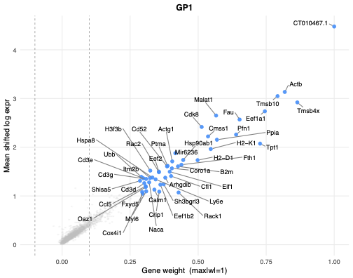
Fig. 2A. “Signature volcano” plot for one example GP (GP1): each gene’s normalized score (x-axis, max |score| = 1) versus its mean shifted-log expression (y-axis), with the top-scoring genes labeled.
(B) Active-cell proportion per GP
# ============================================================
# 2B: histogram of the proportion of highly-active cells per GP
# ============================================================
L_pm_norm_col <- L_pm_filtered / matrix(apply(L_pm_filtered, 2, function(x) max(x)), nrow = nrow(L_pm_filtered), ncol = ncol(L_pm_filtered), byrow = TRUE)
gp_active_cell_counts <- colSums((L_pm_norm_col) > 1e-1)
gp_active_cell_prop <- gp_active_cell_counts / nrow(L_pm_norm_col)
p_2B <- ggplot(data.frame(prop = gp_active_cell_prop), aes(x = prop)) +
  geom_histogram(bins = 40, fill = "steelblue", color = "white") +
  scale_x_log10(labels = scales::label_percent()) +
  annotation_logticks(sides = "b") +
  labs(x = "Proportion of highly active cells per GP (log scale)", y = "Count",
       title = "Histogram of highly active cells per GP (proportion)") +
  theme_minimal(base_size = 13)
ggsave(filename = paste0(figure_path, "2B.pdf"), plot = p_2B, width = 6, height = 4, dpi = 300)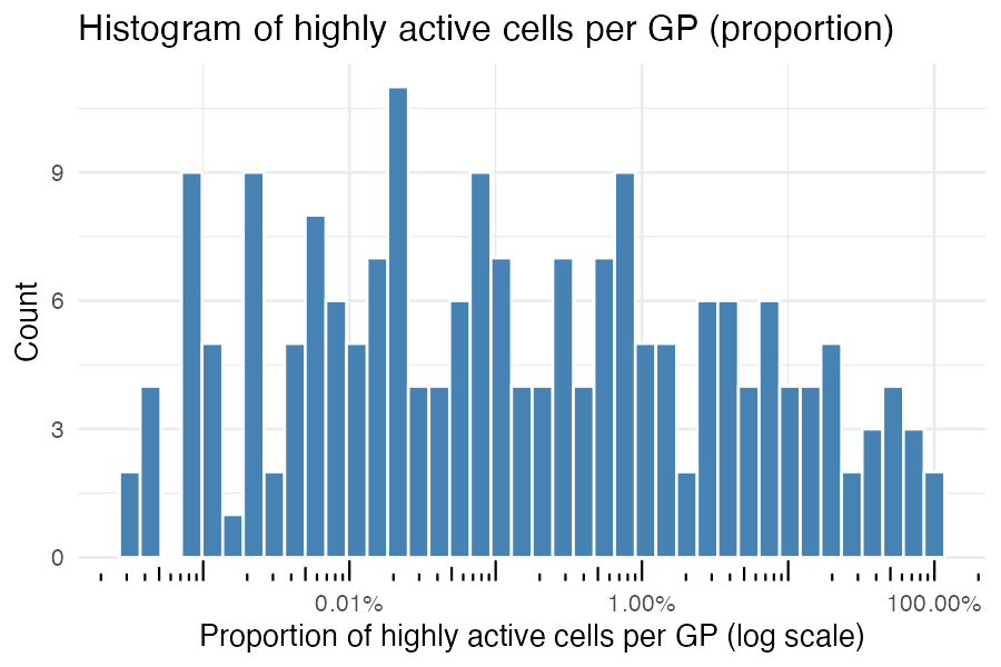
Fig. 2B. Histogram of the proportion of cells with high loading (> 0.1) per GP, across all 200 GPs (x-axis on log scale).
(C) Active-gene count per GP
# ============================================================
# 2C: histogram of the number of highly-active genes per GP
# ============================================================
F_pm_norm_col <- F_pm_filtered / matrix(apply(F_pm_filtered, 2, function(x) max(abs(x))), nrow = nrow(F_pm_filtered), ncol = ncol(F_pm_filtered), byrow = TRUE)
gp_active_gene_counts <- colSums(abs(F_pm_norm_col) > 0.25)
p_2C <- ggplot(data.frame(count = gp_active_gene_counts), aes(x = count)) +
  geom_histogram(bins = 40, fill = "steelblue", color = "white") +
  scale_x_log10(labels = scales::label_comma()) +
  annotation_logticks(sides = "b") +
  labs(x = "Number of highly active genes per GP (log scale)", y = "Count",
       title = "Histogram of highly active genes per GP") +
  theme_minimal(base_size = 13)
ggsave(filename = paste0(figure_path, "2C.pdf"), plot = p_2C, width = 6, height = 4, dpi = 300)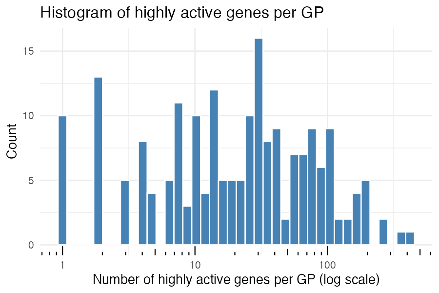
Fig. 2C. Histogram of the number of highly-active genes (|score| > 0.25 of that GP’s max) per GP (x-axis on log scale).
(D) Active-GP count by lineage
# ============================================================
# 2D: boxplot of active-GP-count per cell, by major lineage
# ============================================================
gp_active_cell_counts_level1 <- dplyr::bind_rows(lapply(level1_order, function(grp) {
  cells_grp <- seurat_meta_filtered$cellID[seurat_meta_filtered$annotation_level1 == grp]
  L_grp <- L_pm_filtered[seurat_meta_filtered$cellID %in% cells_grp, , drop = FALSE]
  data.frame(Group = grp, Active_Cell_Counts = rowSums(L_grp > 1e-1))
}))
group_counts <- gp_active_cell_counts_level1 %>%
  group_by(Group) %>% summarise(n = n(), .groups = "drop") %>%
  mutate(Group_Label = paste0(Group, "\n(n=", n, ")")) %>%
  mutate(Group = factor(Group, levels = level1_order)) %>%
  arrange(Group) %>% mutate(Group_Label = factor(Group_Label, levels = Group_Label))
plot_df_g <- gp_active_cell_counts_level1 %>% left_join(group_counts, by = "Group")
p_2D <- ggplot(plot_df_g, aes(x = Group_Label, y = Active_Cell_Counts, fill = Group)) +
  geom_boxplot(outlier.size = 0.4, width = 0.6, alpha = 0.8, color = "gray40") +
  scale_fill_manual(values = ZemmourLib::immgent_colors$level1) +
  labs(title = "Active Gene Programs per Group", x = "Cell Group (Annotation Level 1)", y = "Number of highly active GPs") +
  theme_minimal(base_size = 13) +
  theme(plot.title = element_text(face = "bold", size = 14, hjust = 0.5), axis.text.x = element_text(size = 11, angle = 45, hjust = 1), axis.text.y = element_text(size = 12), axis.title.y = element_text(size = 13, face = "bold"), legend.position = "none", panel.grid.minor = element_blank())
ggsave(filename = paste0(figure_path, "2D.pdf"), plot = p_2D, width = 6, height = 4, dpi = 300)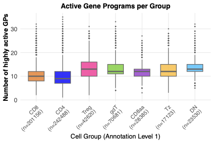
Fig. 2D. Boxplot of the number of active GPs (loading > 0.1) per cell, grouped by major lineage.
(E) Active-GP count, activated vs. resting
# ============================================================
# 2E: boxplot of active-GP-count per cell, activated vs resting
# ============================================================
cells_activated <- seurat_meta_filtered$cellID[seurat_meta_filtered$annotation_level2_group == "activated"]
gp_active_cell_counts_activated <- rowSums(L_pm_filtered[seurat_meta_filtered$cellID %in% cells_activated, ] > 1e-1)
cells_resting <- seurat_meta_filtered$cellID[seurat_meta_filtered$annotation_level2_group == "resting"]
gp_active_cell_counts_resting <- rowSums(L_pm_filtered[seurat_meta_filtered$cellID %in% cells_resting, ] > 1e-1)
gp_active_cell_counts_df <- data.frame(
  Group = c(rep("Activated", length(gp_active_cell_counts_activated)), rep("Resting", length(gp_active_cell_counts_resting))),
  Active_Cell_Counts = c(gp_active_cell_counts_activated, gp_active_cell_counts_resting))
p_2E <- ggplot(gp_active_cell_counts_df, aes(x = Group, y = Active_Cell_Counts, fill = Group)) +
  geom_boxplot(outlier.size = 0.4, width = 0.6, alpha = 0.8, color = "gray40") +
  scale_fill_manual(values = c("Activated" = "#1f78b4", "Resting" = "#e31a1c")) +
  labs(title = "", x = "", y = "Number of highly active GPs") +
  theme_minimal(base_size = 13) +
  theme(plot.title = element_text(face = "bold", size = 14, hjust = 0.5), axis.text.x = element_text(size = 12), axis.text.y = element_text(size = 12), axis.title.y = element_text(size = 13, face = "bold"), legend.position = "none")
ggsave(filename = paste0(figure_path, "2E.pdf"), plot = p_2E, width = 6, height = 4, dpi = 300)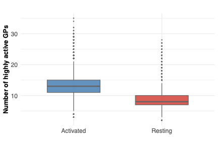
Fig. 2E. Boxplot of the number of active GPs per cell, comparing activated versus resting cells.
(F) CD44 vs. active-GP count
# ============================================================
# 2F: scatter of CD44 protein level vs. number of active GPs per cell
# ============================================================
gp_active_cell_counts_all <- rowSums(L_pm_filtered > 1e-1)
gp_cd44_df <- data.frame(CD44_Protein_Level = protein_mat_normalized_lognorm, Active_GP_Counts = gp_active_cell_counts_all)
gp_cd44_df_nz <- gp_cd44_df %>% dplyr::filter(CD44_Protein_Level > 0)
R <- cor(gp_cd44_df_nz$CD44_Protein_Level, gp_cd44_df_nz$Active_GP_Counts, use = "complete.obs") # on all non-zero-CD44 cells, not just the plotted subsample
set.seed(123)
df_nz <- gp_cd44_df_nz %>% sample_n(min(10000, nrow(.))) # subsample only for scatter rendering
p_2F <- ggplot(df_nz, aes(CD44_Protein_Level, Active_GP_Counts)) +
  geom_point(alpha = 0.1, size = 0.7) +
  geom_smooth(method = "lm", se = TRUE) +
  labs(title = "CD44 Protein Level vs Number of Active GPs", x = "CD44 Protein Level (log-normalized)", y = "Number of Active GPs") +
  annotate("text", x = min(df_nz$CD44_Protein_Level, na.rm = TRUE) + 0.5, y = max(df_nz$Active_GP_Counts, na.rm = TRUE) - 1, label = paste0("R = ", round(R, 2)), size = 4) +
  theme_minimal(base_size = 13)
ggsave(filename = paste0(figure_path, "2F.pdf"), plot = p_2F, width = 6, height = 4, dpi = 300)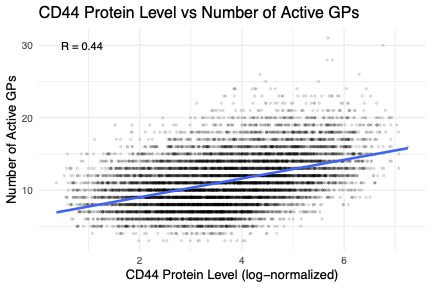
Fig. 2F. Scatter plot of CD44 surface-protein level (log-normalized) against the number of active GPs per cell.
sessionInfo()R version 4.5.1 (2025-06-13)
Platform: aarch64-apple-darwin20
Running under: macOS Sequoia 15.6.1
Matrix products: default
BLAS: /System/Library/Frameworks/Accelerate.framework/Versions/A/Frameworks/vecLib.framework/Versions/A/libBLAS.dylib
LAPACK: /Library/Frameworks/R.framework/Versions/4.5-arm64/Resources/lib/libRlapack.dylib; LAPACK version 3.12.1
locale:
[1] en_CA/en_CA/en_CA/C/en_CA/en_CA
time zone: America/Chicago
tzcode source: internal
attached base packages:
[1] stats graphics grDevices utils datasets methods base
loaded via a namespace (and not attached):
[1] vctrs_0.7.3 cli_3.6.6 knitr_1.50 rlang_1.2.0
[5] xfun_0.55 stringi_1.8.7 otel_0.2.0 promises_1.5.0
[9] jsonlite_2.0.0 workflowr_1.7.2 glue_1.8.1 rprojroot_2.1.1
[13] git2r_0.36.2 htmltools_0.5.9 httpuv_1.6.16 sass_0.4.10
[17] rmarkdown_2.30 evaluate_1.0.5 jquerylib_0.1.4 tibble_3.3.0
[21] fastmap_1.2.0 yaml_2.3.12 lifecycle_1.0.5 whisker_0.4.1
[25] stringr_1.6.0 compiler_4.5.1 fs_1.6.6 Rcpp_1.1.1-1.1
[29] pkgconfig_2.0.3 later_1.4.4 digest_0.6.39 R6_2.6.1
[33] pillar_1.11.1 magrittr_2.0.5 bslib_0.9.0 tools_4.5.1
[37] cachem_1.1.0