Figure 8b: A nonlinear deep-learning framework independently recovers the immgenT gene-program landscape

workflowr

• Summary
• Checks
• Past versions

Last updated: 2026-09-10

Checks: 7 0

Knit directory: immgenT-GP-analysis/analysis/

This reproducible R Markdown analysis was created with workflowr (version 1.7.2). The Checks tab describes the reproducibility checks that were applied when the results were created. The Past versions tab lists the development history.

---

R Markdown file: up-to-date

Great! Since the R Markdown file has been committed to the Git repository, you know the exact version of the code that produced these results.

Environment: empty

Great job! The global environment was empty. Objects defined in the global environment can affect the analysis in your R Markdown file in unknown ways. For reproduciblity it’s best to always run the code in an empty environment.

Seed: set.seed(1)

The command set.seed(1) was run prior to running the code in the R Markdown file. Setting a seed ensures that any results that rely on randomness, e.g. subsampling or permutations, are reproducible.

Session information: recorded

Great job! Recording the operating system, R version, and package versions is critical for reproducibility.

Cache: none

Nice! There were no cached chunks for this analysis, so you can be confident that you successfully produced the results during this run.

File paths: relative

Great job! Using relative paths to the files within your workflowr project makes it easier to run your code on other machines.

Repository version: 59146f9

Great! You are using Git for version control. Tracking code development and connecting the code version to the results is critical for reproducibility.

The results in this page were generated with repository version 59146f9. See the Past versions tab to see a history of the changes made to the R Markdown and HTML files.

Note that you need to be careful to ensure that all relevant files for the analysis have been committed to Git prior to generating the results (you can use wflow_publish or wflow_git_commit). workflowr only checks the R Markdown file, but you know if there are other scripts or data files that it depends on. Below is the status of the Git repository when the results were generated:

Ignored files:
    Ignored:    .DS_Store
    Ignored:    .claude/
    Ignored:    analysis/.DS_Store
    Ignored:    analysis/.Rhistory
    Ignored:    analysis/assets/.DS_Store
    Ignored:    captions/
    Ignored:    code/.DS_Store
    Ignored:    code/other/topic_flashier_20250212.R
    Ignored:    code/other/topic_wrapper_20250215_alldata_backfit.sh
    Ignored:    data
    Ignored:    experiments/
    Ignored:    figures/.DS_Store
    Ignored:    figures/final-selected/.DS_Store
    Ignored:    figures/final-selected/Figure 1/.DS_Store
    Ignored:    figures/final-selected/Figure 2/.DS_Store
    Ignored:    figures/final-selected/Figure 5/.DS_Store
    Ignored:    figures/final-selected/Figure S1/.DS_Store
    Ignored:    internal/
    Ignored:    log/
    Ignored:    output/.DS_Store
    Ignored:    output/Figure2/
    Ignored:    plan/
    Ignored:    tables/
    Ignored:    tmp/

Note that any generated files, e.g. HTML, png, CSS, etc., are not included in this status report because it is ok for generated content to have uncommitted changes.

---

These are the previous versions of the repository in which changes were made to the R Markdown (analysis/Figure8.Rmd) and HTML (docs/Figure8.html) files. If you’ve configured a remote Git repository (see ?wflow_git_remote), click on the hyperlinks in the table below to view the files as they were in that past version.

File	Version	Author	Date	Message
html	60125af	Ziang Zhang	2026-09-10	Build site: Figure 4b on the shared column colours
html	88ee847	Ziang Zhang	2026-09-10	Build site: Figure 4b without the miniverse clusters
html	5874416	Ziang Zhang	2026-09-10	Build site: main Figure 4 inserted, Extended Data back to 1-7
Rmd	4307b28	Ziang Zhang	2026-09-10	New main Figure 4, and fold the cluster heatmap into Extended Data Figure 2

---

This page documents Figure 8b. The other panels of Figure 8 (A nonlinear deep-learning framework independently recovers the immgenT gene-program landscape) are produced by the RQVI framework and are documented in the companion repository for RQVI.

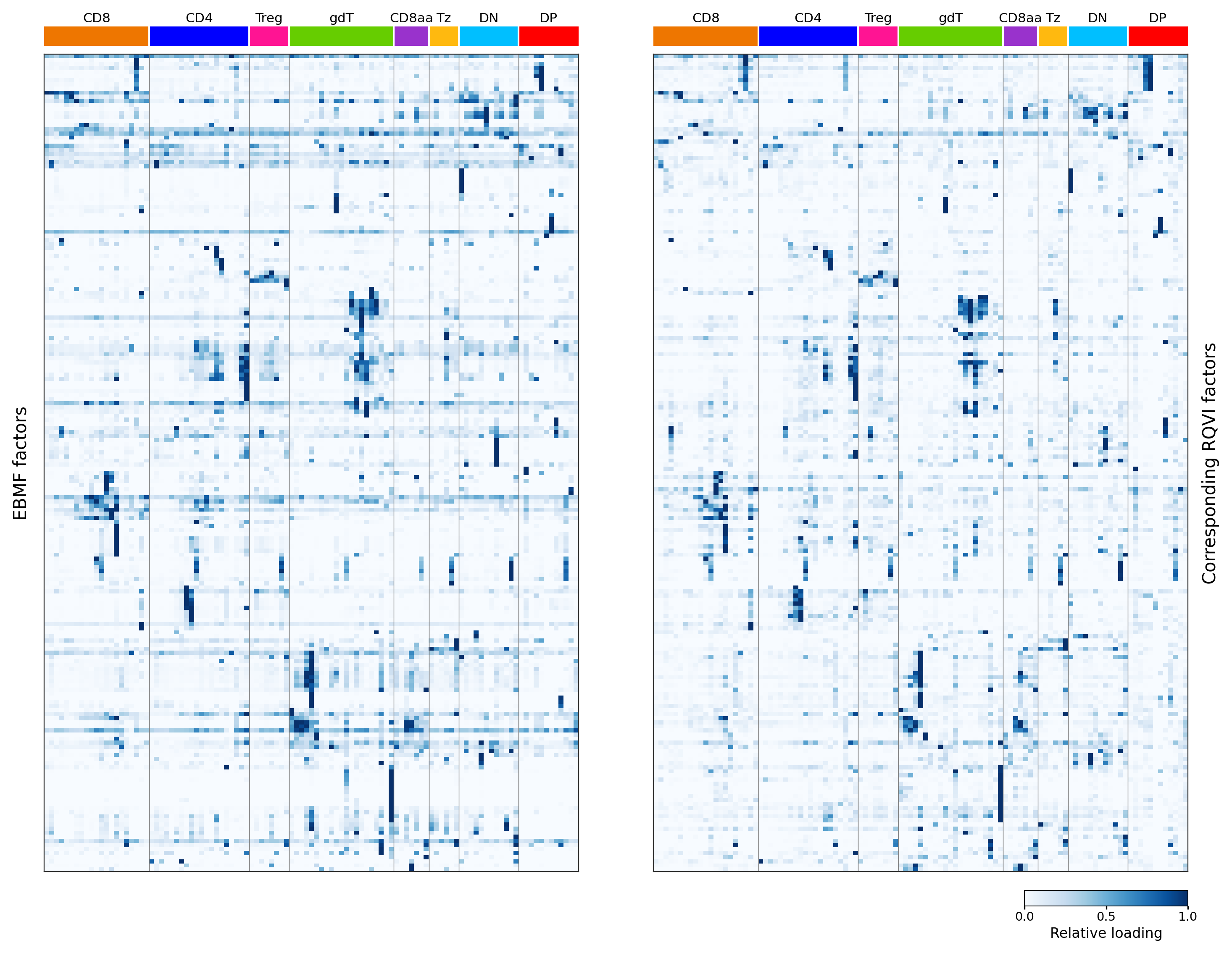
Figure 8b asks whether the fine-grained cluster-level patterns captured by the 200 EBMF GPs are recovered by an independent factorization. It compares each EBMF GP with a matched RQVI GP – RQVI being an alternative matrix factorization of the same cells, run across 10 random-seed initializations (256 GPs per seed). The two heatmaps share the same row and column order and use a white-to-blue scale of per-GP relative loading on [0, 1], with broad lineage annotations above the columns.

Cells are the L_pm_filtered GP loadings (cells passing the iterative total-loading filter), restricted to non-thymocytes (annotation_level1 != "thymocyte", all conditions) and to cells that also carry an RQVI loading. EBMF and RQVI loadings are averaged within annotation_level2 on these common cells, and each RQVI GP is shown on the row of its matched EBMF GP. In the code and in the intermediate files the EBMF GPs are named F1-F200; those are GP1-GP200.

Figure 8b

Past versions of 8B.png

Version	Author	Date
5874416	Ziang Zhang	2026-09-10

Fig. 8b. Cluster-level activity profiles of corresponding EBMF and RQVI GPs. EBMF cell loadings (left) and matched RQVI program loadings (right) were averaged within the 107 level-2 clusters.

How the figure is made

Three steps, run from the repository root:

Rscript script/Figure8b.R          # cluster-mean matrices + column/palette metadata
python  script/Figure8b_rematch.py # one-to-one EBMF-RQVI program matching
python  script/Figure8b_plot.py    # heatmaps

The Python steps require matplotlib, pandas, scipy, h5py, and numpy. The RQVI cell-level loadings are read as input from data/, which is a git-ignored symlink and is not tracked here.

Cluster means

script/Figure8b.R builds the raw annotation_level2 cluster-mean matrix for the EBMF GPs on the common non-thymocyte cells, together with the column order (Figure-1 level1 lineage order, alphabetical within each lineage) and the lineage color palette. The matched RQVI cluster means are produced by the matching step below.

# Figure 8b (data step): EBMF cluster-mean matrix and column/palette metadata for
# the EBMF vs RQVI gene-program comparison across annotation_level2 clusters.
#
#   * Cells: L_pm_filtered gene-program loadings (cells passing the iterative
#     total-loading filter), restricted to non-thymocytes (annotation_level1 !=
#     "thymocyte", all conditions) and to cells that also carry an RQVI loading
#     ("common cells"). The RQVI cell set is taken from the cell_id index of the
#     RQVI loading table.
#   * EBMF matrix: flashier loadings L_pm_filtered (GP1..GP200), averaged within
#     annotation_level2 on the common cells.
#   * Columns (level2 clusters) are ordered by the Figure-1 level1 lineage order,
#     alphabetically within each lineage.
#
# This script writes the EBMF cluster-mean matrix, a cell->annotation table, and
# the column order + lineage palette. The RQVI cluster means and the one-to-one
# EBMF-RQVI matching are computed by script/Figure8b_rematch.py; row ordering,
# per-program [0,1] scaling, and the heatmaps by script/Figure8b_plot.py.

suppressPackageStartupMessages({
  library(arrow)
  library(data.table)
  library(ZemmourLib)
})

if (!file.exists("code/R/setup_data.R")) {
  stop("Run this script from the immgenT-GP-analysis repository root.")
}
source("code/R/setup_data.R")

outdir <- "output/Figure8b"   # build intermediates; final panels come from Figure8b_plot.py
dir.create(outdir, recursive = TRUE, showWarnings = FALSE)

PKG <- "data/rqvi_loading/RQVI_EBMF_heatmap_data_v1/data"
rqvi_loading_path <- file.path(PKG, "rqvi_matched_200_cell_loadings.parquet")
level1_order <- c("CD8", "CD4", "Treg", "gdT", "CD8aa", "Tz", "DN", "DP")

## ---- EBMF loadings + metadata ----
gp <- load_gp_data()
L  <- gp$L_pm_filtered
colnames(L) <- paste0("GP", seq_len(ncol(L)))
meta <- gp$seurat_meta_filtered
stopifnot(identical(rownames(L), rownames(meta)), ncol(L) == 200L)

nonthy <- meta$annotation_level1 != "thymocyte"
if (anyNA(nonthy)) stop("annotation_level1 has missing values.")

## ---- common cells (non-thymocyte, in L_pm, and with an RQVI loading) ----
rqvi_cell_ids <- as.data.frame(arrow::read_parquet(rqvi_loading_path, col_select = "cell_id"))$cell_id
our_nonthy_ids <- rownames(L)[nonthy]
common_ids <- our_nonthy_ids[our_nonthy_ids %in% rqvi_cell_ids]
grp <- droplevels(factor(as.character(meta$annotation_level2[match(common_ids, rownames(meta))])))
if (anyNA(grp) || any(as.character(grp) == "")) stop("Missing level2 labels on common cells.")

message(sprintf("common non-thymocyte cells: %d (healthy %d / non-healthy %d); level2 clusters: %d",
                length(common_ids),
                sum(meta$condition_broad[match(common_ids, rownames(meta))] == "healthy"),
                sum(meta$condition_broad[match(common_ids, rownames(meta))] != "healthy"),
                nlevels(grp)))

## ---- EBMF cluster means (columns F1..F200) ----
Lc <- L[common_ids, , drop = FALSE]
colnames(Lc) <- paste0("F", seq_len(ncol(Lc)))
esum <- rowsum(Lc, grp)
ecnt <- as.integer(table(grp)[rownames(esum)])
ebmf_means <- sweep(esum, 1L, ecnt, "/")                 # K x 200
stopifnot(nrow(ebmf_means) == 107L, ncol(ebmf_means) == 200L)

## ---- level2 column order (Figure-1 level1 order, alphabetical within) ----
l2  <- rownames(ebmf_means)
lmap <- unique(data.frame(level2 = as.character(meta$annotation_level2),
                          level1 = as.character(meta$annotation_level1),
                          stringsAsFactors = FALSE))
if (anyDuplicated(lmap$level2)) stop("A level2 label maps to multiple level1 labels.")
lin <- lmap$level1[match(l2, lmap$level2)]
if (anyNA(lin) || !all(lin %in% level1_order)) stop("Unexpected level1 lineage among clusters.")
ord <- order(match(lin, level1_order), l2)
cluster_order <- data.frame(
  level2_cluster = l2[ord],
  level1         = lin[ord],
  display_column = seq_along(ord) - 1L,
  n_cells        = ecnt[ord],
  stringsAsFactors = FALSE
)

## ---- level1 palette (canonical lineage colors) as hex ----
l1pal <- ZemmourLib::immgent_colors$level1
hex <- vapply(l1pal, function(cc) {
  v <- grDevices::col2rgb(cc)
  grDevices::rgb(v[1], v[2], v[3], maxColorValue = 255)
}, character(1))
pal_df <- data.frame(level1 = names(hex), color = unname(hex), stringsAsFactors = FALSE)

## ---- write outputs ----
# cell -> level1/level2 for all L_pm_filtered cells; consumed by Figure8b_rematch.py
# to define common cells and clusters (avoids any machine-specific path).
fwrite(data.frame(
  cellID            = rownames(L),
  annotation_level1 = as.character(meta$annotation_level1),
  annotation_level2 = as.character(meta$annotation_level2),
  stringsAsFactors  = FALSE
), file.path(outdir, "8b_cell_metadata.csv.gz"))

fwrite(data.frame(level2_cluster = rownames(ebmf_means), ebmf_means, check.names = FALSE),
       file.path(outdir, "8b_ebmf_raw_means_level2.csv"))
fwrite(cluster_order, file.path(outdir, "8b_cluster_order.csv"))
fwrite(pal_df,        file.path(outdir, "8b_level1_palette.csv"))
fwrite(data.frame(
  metric = c("common_cells", "healthy_cells", "nonhealthy_cells", "level2_clusters", "ebmf_factors"),
  value  = c(length(common_ids),
             sum(meta$condition_broad[match(common_ids, rownames(meta))] == "healthy"),
             sum(meta$condition_broad[match(common_ids, rownames(meta))] != "healthy"),
             nlevels(grp), 200L)
), file.path(outdir, "8b_build_summary.csv"))

message("Wrote Fig S5 data inputs to ", normalizePath(outdir))

Matching

Each GP’s mean-loading profile is z-scored across clusters; the signed Pearson correlation between every EBMF GP and all 2,560 candidate RQVI GPs is computed; candidates with a constant profile are excluded; and a maximum-weight one-to-one assignment (scipy.optimize.linear_sum_assignment) matches each EBMF GP to a distinct RQVI GP so that the total signed correlation is maximized. The assignment is computed over all common cells (108 annotation_level2 clusters); the figure displays the 107 non-thymocyte clusters. The median per-GP correlation is 0.766, with 92.5% at r >= 0.5. Code: script/Figure8b_rematch.py.

Plotting

script/Figure8b_plot.py orders the EBMF rows by hierarchical clustering (average linkage, correlation distance, optimal leaf ordering), rescales every GP to [0, 1] across clusters, and draws the two heatmaps with a shared colorbar; the matched RQVI panel reuses the EBMF row order. The published PDF and the PNG this page shows come out of the same matplotlib figure in one call, so the two cannot drift apart. Code: script/Figure8b_plot.py.

Session information

sessionInfo()

R version 4.5.1 (2025-06-13)
Platform: aarch64-apple-darwin20
Running under: macOS Sequoia 15.6.1

Matrix products: default
BLAS:   /System/Library/Frameworks/Accelerate.framework/Versions/A/Frameworks/vecLib.framework/Versions/A/libBLAS.dylib 
LAPACK: /Library/Frameworks/R.framework/Versions/4.5-arm64/Resources/lib/libRlapack.dylib;  LAPACK version 3.12.1

locale:
[1] en_CA/en_CA/en_CA/C/en_CA/en_CA

time zone: America/Chicago
tzcode source: internal

attached base packages:
[1] stats     graphics  grDevices utils     datasets  methods   base     

loaded via a namespace (and not attached):
 [1] vctrs_0.7.3     cli_3.6.6       knitr_1.50      rlang_1.2.0    
 [5] xfun_0.55       stringi_1.8.9   otel_0.2.0      promises_1.5.0 
 [9] jsonlite_2.0.0  workflowr_1.7.2 glue_1.8.1      rprojroot_2.1.1
[13] git2r_0.36.2    htmltools_0.5.9 httpuv_1.6.16   sass_0.4.10    
[17] rmarkdown_2.30  evaluate_1.0.5  jquerylib_0.1.4 tibble_3.3.0   
[21] fastmap_1.2.0   yaml_2.3.12     lifecycle_1.0.5 whisker_0.4.1  
[25] stringr_1.6.0   compiler_4.5.1  fs_1.6.6        Rcpp_1.1.1-1.1 
[29] pkgconfig_2.0.3 later_1.4.4     digest_0.6.39   R6_2.6.1       
[33] pillar_1.11.1   magrittr_2.0.5  bslib_0.9.0     tools_4.5.1    
[37] cachem_1.1.0