Extended Data Figure 3: Activation-associated GPs
Ziang Zhang
Last updated: 2026-09-10
Checks: 7 0
Knit directory:
immgenT-GP-analysis/analysis/
This reproducible R Markdown analysis was created with workflowr (version 1.7.2). The Checks tab describes the reproducibility checks that were applied when the results were created. The Past versions tab lists the development history.
Great! Since the R Markdown file has been committed to the Git repository, you know the exact version of the code that produced these results.
Great job! The global environment was empty. Objects defined in the global environment can affect the analysis in your R Markdown file in unknown ways. For reproduciblity it’s best to always run the code in an empty environment.
The command set.seed(1) was run prior to running the
code in the R Markdown file. Setting a seed ensures that any results
that rely on randomness, e.g. subsampling or permutations, are
reproducible.
Great job! Recording the operating system, R version, and package versions is critical for reproducibility.
Nice! There were no cached chunks for this analysis, so you can be confident that you successfully produced the results during this run.
Great job! Using relative paths to the files within your workflowr project makes it easier to run your code on other machines.
Great! You are using Git for version control. Tracking code development and connecting the code version to the results is critical for reproducibility.
The results in this page were generated with repository version 59146f9. See the Past versions tab to see a history of the changes made to the R Markdown and HTML files.
Note that you need to be careful to ensure that all relevant files for
the analysis have been committed to Git prior to generating the results
(you can use wflow_publish or
wflow_git_commit). workflowr only checks the R Markdown
file, but you know if there are other scripts or data files that it
depends on. Below is the status of the Git repository when the results
were generated:
Ignored files:
    Ignored:    .DS_Store
    Ignored:    .claude/
    Ignored:    analysis/.DS_Store
    Ignored:    analysis/.Rhistory
    Ignored:    analysis/assets/.DS_Store
    Ignored:    captions/
    Ignored:    code/.DS_Store
    Ignored:    code/other/topic_flashier_20250212.R
    Ignored:    code/other/topic_wrapper_20250215_alldata_backfit.sh
    Ignored:    data
    Ignored:    experiments/
    Ignored:    figures/.DS_Store
    Ignored:    figures/final-selected/.DS_Store
    Ignored:    figures/final-selected/Figure 1/.DS_Store
    Ignored:    figures/final-selected/Figure 2/.DS_Store
    Ignored:    figures/final-selected/Figure 5/.DS_Store
    Ignored:    figures/final-selected/Figure S1/.DS_Store
    Ignored:    internal/
    Ignored:    log/
    Ignored:    output/.DS_Store
    Ignored:    output/Figure2/
    Ignored:    plan/
    Ignored:    tables/
    Ignored:    tmp/
Note that any generated files, e.g. HTML, png, CSS, etc., are not included in this status report because it is ok for generated content to have uncommitted changes.
These are the previous versions of the repository in which changes were
made to the R Markdown (analysis/FigureS3.Rmd) and HTML
(docs/FigureS3.html) files. If you’ve configured a remote
Git repository (see ?wflow_git_remote), click on the
hyperlinks in the table below to view the files as they were in that
past version.
| File | Version | Author | Date | Message |
|---|---|---|---|---|
| html | 60125af | Ziang Zhang | 2026-09-10 | Build site: Figure 4b on the shared column colours |
| html | 88ee847 | Ziang Zhang | 2026-09-10 | Build site: Figure 4b without the miniverse clusters |
| html | 5874416 | Ziang Zhang | 2026-09-10 | Build site: main Figure 4 inserted, Extended Data back to 1-7 |
| Rmd | 4307b28 | Ziang Zhang | 2026-09-10 | New main Figure 4, and fold the cluster heatmap into Extended Data Figure 2 |
| html | bf4f612 | Ziang Zhang | 2026-09-09 | Build site: Extended Data back to 1-8 |
| Rmd | 6f01135 | Ziang Zhang | 2026-09-09 | Pull the tissue figure back out of Extended Data; ED is 1-8 again |
| html | a7a481f | Ziang Zhang | 2026-09-09 | Build site: the rebuilt Figure 1d and the Extended Data renumbering |
| Rmd | c233cd8 | Ziang Zhang | 2026-09-09 | Extended Data reorganisation: split the tissue/cluster figure, renumber 3-8 |
| html | 1e88d7e | Ziang Zhang | 2026-09-04 | Build site: published captions and titles across all 24 pages |
| Rmd | 0267e5b | Ziang Zhang | 2026-09-04 | Captions from the published manuscript; trim editor notes off the page code |
| html | 19c977f | Ziang Zhang | 2026-09-02 | Build site: Extended Data 5-7 renumbered, Figure S5 page rebuilt |
| html | 9167d8f | Ziang Zhang | 2026-08-19 | Build site: Extended Data Figure 3 page rebuilt |
| Rmd | 7b0f736 | Ziang Zhang | 2026-08-19 | Extended Data Figure 3 intro: drop the repository-scope phrasing |
| html | ae03072 | Ziang Zhang | 2026-08-19 | Build site: six pages rebuilt after the prose cleanup |
| Rmd | adc2327 | Ziang Zhang | 2026-08-19 | Site prose: finish taking internal notes off the pages |
| html | eeca07b | Ziang Zhang | 2026-08-05 | Keep pre-refactor provenance in panel comments off the published pages |
| Rmd | 5651d0e | Ziang Zhang | 2026-08-05 | Extended Data tables: reorder to six, rebuild Table 1, drop internal notes |
| html | cbcec52 | Ziang Zhang | 2026-07-30 | Build site: Extended Data Figure naming |
| Rmd | 66aa029 | Ziang Zhang | 2026-07-30 | Name the Extended Data figures as published on the site |
| html | ac650a0 | Ziang Zhang | 2026-07-30 | Build site: Figure S5 (ex-S6a) and Figure S6 as a-f |
| html | ae21d37 | Ziang Zhang | 2026-07-28 | Build site: republish after the reorder commits |
| html | d538aa2 | Ziang Zhang | 2026-07-28 | Build site: reordered Figures 6 / S6 / S3 and the new Figure 7b page |
| Rmd | 4c07670 | Ziang Zhang | 2026-07-28 | Reorder Figures 6, S6 and S3; make the ex-S5 figure Figure 7b |
| html | 029b0ae | Ziang Zhang | 2026-07-28 | Build site. |
| Rmd | 0f5b5da | Ziang Zhang | 2026-07-28 | Align all figure captions with captions_20260728_final.docx |
| html | 3fc3789 | Ziang Zhang | 2026-07-27 | Republish all 24 pages |
| html | 1390a03 | Ziang Zhang | 2026-07-27 | Republish all 24 pages |
| html | adaef21 | Ziang Zhang | 2026-07-27 | Build site: panel fixes and PDF-derived assets |
| html | 5b19858 | Ziang Zhang | 2026-07-27 | Build site. |
| Rmd | 91ee059 | Ziang Zhang | 2026-07-26 | Select each panel’s code block by name, not by line number |
| html | 91ee059 | Ziang Zhang | 2026-07-26 | Select each panel’s code block by name, not by line number |
| Rmd | fa5a501 | Ziang Zhang | 2026-07-18 | Fig S3c: reproduce collaborator panel (activated CD4/CD8, threshold 0.1) |
| html | fa5a501 | Ziang Zhang | 2026-07-18 | Fig S3c: reproduce collaborator panel (activated CD4/CD8, threshold 0.1) |
| Rmd | b197499 | Ziang Zhang | 2026-07-16 | Restructure main figures (renumber + split Figure 1) |
| html | b197499 | Ziang Zhang | 2026-07-16 | Restructure main figures (renumber + split Figure 1) |
| html | 92021bf | Ziang Zhang | 2026-07-02 | Build site. |
| html | 827c89b | Ziang Zhang | 2026-07-02 | Build site. |
| Rmd | 8ac7f9f | Ziang Zhang | 2026-07-02 | Add data provenance notes to each script; remove conversational |
| Rmd | f9db962 | Ziang Zhang | 2026-07-02 | Simplify layout: drop old code/script folders, rename |
| html | c6e5086 | Ziang Zhang | 2026-07-02 | Build site. |
| html | 5a79883 | Ziang Zhang | 2026-07-02 | Build site. |
| Rmd | 2b0e445 | Ziang Zhang | 2026-07-02 | Fix GitHub source links to point at the new |
| html | cf1d0ac | Ziang Zhang | 2026-07-02 | Build site. |
| Rmd | 06b2461 | Ziang Zhang | 2026-07-02 | Initial commit: immgenT-GP-analysis |
| html | 06b2461 | Ziang Zhang | 2026-07-02 | Initial commit: immgenT-GP-analysis |
Panels (b)-(f) are produced by script/FigureS3.R,
which shares its curated GP set with Figure 5
via code/R/activation_shared_setup.R. The code below is
shown for reference (not re-executed on this page); the images are its
pre-rendered output.
Panel (a) is not generated from code – see below.
Setup
# Figure S3. Characterizing activation GPs.
#
# Panels produced:
#
# s3a is the definition of resting vs activated CD4/CD8 cells (the
# lineage-specific MDEs plus the adjacent CD62L-vs-CD44 protein plot, one
# panel). It is NOT produced here -- no code in this repository draws it; see
# analysis/FigureS3.Rmd.
#
#   s3b  Fraction of activated CD4/CD8 cells per organ with GP26 > 0.1, sorted.
#   s3c  GSEA dot plot relating the activation GPs to curated gene sets.
#   s3d  Fraction of activated CD4 cells with GP79 loading > 0.1, by condition.
#   s3e  Per-cell log2FC heatmap of activation GPs vs resting baseline.
#   s3f  Fraction of activated CD8/CD4 cells with GP57 loading > 0.1: cancer
#        vs all other conditions.
#
# The curated GP set and activated/resting cell groupings are shared with
# Figure 5 via code/R/activation_shared_setup.R.
#
# Panel s3b is computed on activated CD4/CD8 cells only (annotation_level1 in
# {CD4, CD8} and annotation_level2_group == "activated"): the per-organ fraction
# with GP26 loading > 0.1.
#
# Required inputs (data/) -- see code/README.md's "Data provenance" table
# for the full picture:
#   L_pm_filtered.rds, F_pm_filtered.rds     [code/pipeline/01b_filter_cells.R]
#   igt1_96_..._ADTonly.Rds                  [primary input Seurat object]
#   GSEA_signatures_select_toplot.csv        [external: curated gene-set collection]

library(ggplot2)
library(dplyr)
library(stringr)
library(pheatmap)
library(scales)

data_path <- "data/"
figure_path <- "figures/final-selected/Figure S3/"
source("code/R/plot_utils.R") # scale_cols()

# ============================================================
# Load data
# ============================================================
L_pm_filtered <- readRDS(paste0(data_path, "L_pm_filtered.rds"))
colnames(L_pm_filtered) <- paste0("GP", seq_len(ncol(L_pm_filtered)))
F_pm_filtered <- readRDS(paste0(data_path, "F_pm_filtered.rds"))
colnames(F_pm_filtered) <- paste0("GP", seq_len(ncol(F_pm_filtered)))
seurat_meta <- readRDS(paste0(data_path, "igt1_96_withtotalvi20260206_clean_ADTonly.Rds"))@meta.data
seurat_meta_filtered <- seurat_meta[rownames(L_pm_filtered), ]
df_sig <- read.csv(paste0(data_path, "GSEA_signatures_select_toplot.csv"), header = TRUE, sep = ",")

source("code/R/activation_shared_setup.R")
(a) Definition of resting and activated CD4/CD8 cells
This panel shows the CITE-seq gating used to define resting and activated cells; it is not generated from code, so only its caption is given here.
Extended Data Fig. 3a. Definition of resting and activated CD4+ and CD8+ T cells. Activated CD44⁺CD62L⁻ (top) and resting CD62L⁺CD44⁻ (bottom) cells are highlighted in each lineage-specific MDE. Gated cells are shown in the adjacent CD62L versus CD44 protein-expression plot (CITE-seq, log-normalized counts).
The annotation_level2_group “activated”/“resting” labels
that every other panel on this page (and all of Figure 5) filters on are the labels this panel
defines, so the gate itself is already in use here – only the figure
illustrating it is absent.
(b) GP26+ rate by organ
# ============================================================
# s3b: Fraction of activated CD4/CD8 cells per organ with GP26 loading > 0.1
# ============================================================
act_cd4_cd8 <- seurat_meta_filtered$annotation_level1 %in% c("CD4", "CD8") &
  seurat_meta_filtered$annotation_level2_group == "activated"
gp26_organ_df <- data.frame(
  organ = seurat_meta_filtered$organ_simplified[act_cd4_cd8],
  gp26_high = L_pm_filtered[act_cd4_cd8, "GP26"] > 0.1
) %>%
  filter(!is.na(organ), organ != "") %>%
  group_by(organ) %>%
  summarise(n_cells = n(), proportion_gp26_high = mean(gp26_high), .groups = "drop") %>%
  arrange(desc(proportion_gp26_high)) %>%
  mutate(organ = factor(organ, levels = organ),
         pct = 100 * proportion_gp26_high,
         pct_lab = sub("\\.0%$", "%", sprintf("%.1f%%", pct)))  # e.g. 99%, 98.7%

# abbreviate a few long organ names to match the published panel
organ_abbrev <- c("submandibular gland" = "submand. gland",
                  "mammary gland"       = "mam. gland",
                  "small intestine epi" = "sm intestine epi",
                  "small intestine LP"  = "sm intestine LP",
                  "peritoneal cavity"   = "perit. cav.")

p_s3b <- ggplot(gp26_organ_df, aes(x = organ, y = pct)) +
  geom_col(fill = "#4C72B0", width = 0.7) +
  geom_text(aes(label = pct_lab), vjust = -0.4, size = 3, color = "grey20") +
  scale_x_discrete(labels = function(x) ifelse(x %in% names(organ_abbrev), organ_abbrev[x], x)) +
  scale_y_continuous(breaks = c(0, 50, 100), labels = c("0", "50%", "100"),
                     expand = expansion(mult = c(0, 0.10))) +
  labs(x = NULL, y = "Proportion activated (loading > 0.1) (%)",
       title = "Activation of GP26 (threshold = 0.1) across Organ") +
  theme_classic(base_size = 12) +
  theme(axis.text.x = element_text(angle = 45, hjust = 1),
        plot.title = element_text(hjust = 0.5))
ggsave(filename = paste0(figure_path, "s3b.pdf"), plot = p_s3b, width = 9, height = 4.8)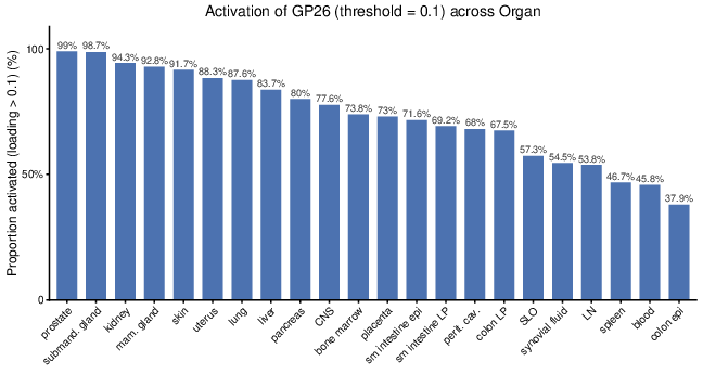
Extended Data Fig. 3b. Bar plot showing broad GP26 activity in activated CD4+ and CD8+ T cells across organs (percent of cells with GP26 activity above 0.1 per tissue)
(c) GSEA dot plot
# ============================================================
# s3c: GSEA dot plot for the activation GPs
# ============================================================
df_sig <- df_sig %>% mutate(factor = str_replace(factor, "^F", "GP"))
present_GPs <- intersect(ordered_GPs, unique(df_sig$factor))
y_levels <- rev(present_GPs) # first GP (GP56) appears at the top of the y-axis
df_plot <- df_sig %>%
  filter(factor %in% present_GPs) %>%
  mutate(pathway = factor(pathway, levels = unique(pathway)), factor = factor(factor, levels = y_levels), log10padj = -log10(padj))
y_factors <- levels(df_plot$factor)
y_colors <- highlight_colors[y_factors]

p_s3c <- ggplot(df_plot, aes(x = pathway, y = factor)) +
  geom_point(aes(size = NES, color = log10padj)) +
  scale_color_viridis_c(name = "-log10(p-adj)") +
  scale_size(range = c(3, 10)) +
  theme_bw() +
  theme(axis.text.x = element_text(angle = 90, hjust = 1), axis.text.y = element_text(color = y_colors, face = "bold")) +
  labs(size = "NES", x = "Pathway", y = "Gene Program")
ggsave(filename = paste0(figure_path, "s3c.pdf"), plot = p_s3c, width = 8, height = 10)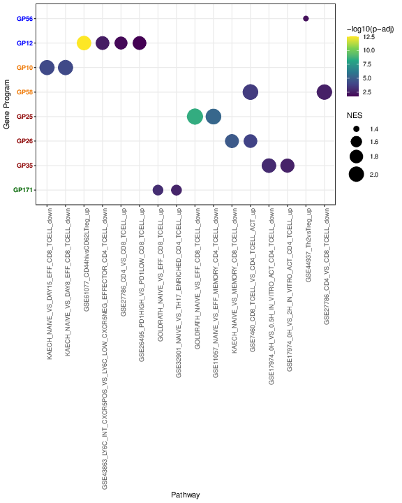
| Version | Author | Date |
|---|---|---|
| 5874416 | Ziang Zhang | 2026-09-10 |
| c233cd8 | Ziang Zhang | 2026-09-09 |
| d538aa2 | Ziang Zhang | 2026-07-28 |
| 7102598 | Ziang Zhang | 2026-07-27 |
| 6c1a613 | Ziang Zhang | 2026-07-27 |
| bf7afcf | Ziang Zhang | 2026-07-27 |
| ea3ecc2 | Ziang Zhang | 2026-07-27 |
| fa5a501 | Ziang Zhang | 2026-07-18 |
| 78e3bba | Ziang Zhang | 2026-07-03 |
| 06b2461 | Ziang Zhang | 2026-07-02 |
Extended Data Fig. 3c. Gene set enrichment analysis (GSEA) dot plot relating activation-associated GPs to curated immunologic signature gene sets. Color denotes −log10 adjusted P value, and dot size denotes the normalized enrichment score (NES).
(d) GP79+ rate across conditions
# ============================================================
# s3d: GP79 high-loading proportion across conditions, activated CD4 cells
# ============================================================
min_cells_gp79_condition <- 50
gp79_cd4_condition_df <- data.frame(
  condition_broad = as.character(seurat_meta_filtered$condition_broad),
  condition_detailed_simplified = as.character(seurat_meta_filtered$condition_detailed_simplified),
  lineage = seurat_meta_filtered$annotation_level1,
  activation_group = seurat_meta_filtered$annotation_level2_group,
  gp79_loading = L_pm_filtered[, "GP79"],
  stringsAsFactors = FALSE
) %>%
  filter(lineage == "CD4", activation_group == "activated", !is.na(condition_detailed_simplified), condition_detailed_simplified != "") %>%
  mutate(gp79_high = gp79_loading > 0.1)

gp79_cd4_condition_summary <- gp79_cd4_condition_df %>%
  group_by(condition_detailed_simplified) %>%
  summarise(
    condition_broad = names(sort(table(condition_broad), decreasing = TRUE))[1],
    n_cells = n(), n_gp79_high = sum(gp79_high), proportion_gp79_high = mean(gp79_high), .groups = "drop"
  ) %>%
  mutate(included_in_plot = n_cells >= min_cells_gp79_condition) %>%
  arrange(desc(proportion_gp79_high), condition_detailed_simplified)

gp79_cd4_condition_plot_df <- gp79_cd4_condition_summary %>%
  filter(included_in_plot) %>%
  arrange(proportion_gp79_high, condition_detailed_simplified) %>%
  mutate(condition_label = factor(condition_detailed_simplified, levels = condition_detailed_simplified))

gp79_broad_levels <- sort(unique(gp79_cd4_condition_plot_df$condition_broad))
gp79_broad_colors <- setNames(scales::hue_pal()(length(gp79_broad_levels)), gp79_broad_levels)
gp79_xmax <- max(gp79_cd4_condition_plot_df$proportion_gp79_high, na.rm = TRUE)
gp79_xmax <- ifelse(gp79_xmax > 0, gp79_xmax, 0.05)
gp79_label_pad <- gp79_xmax * 0.015
gp79_plot_height <- max(7, 0.18 * nrow(gp79_cd4_condition_plot_df) + 2)

p_s3d <- ggplot(gp79_cd4_condition_plot_df, aes(x = proportion_gp79_high, y = condition_label, fill = condition_broad)) +
  geom_col(width = 0.75, color = "grey25", linewidth = 0.2) +
  geom_text(aes(x = proportion_gp79_high + gp79_label_pad, label = scales::percent(proportion_gp79_high, accuracy = 1)), hjust = 0, size = 2.7) +
  scale_x_continuous(labels = scales::percent_format(accuracy = 10), expand = expansion(mult = c(0, 0.02))) +
  scale_fill_manual(values = gp79_broad_colors) +
  coord_cartesian(xlim = c(0, gp79_xmax * 1.15), clip = "off") +
  labs(
    x = "Proportion of activated CD4 cells with GP79 loading > 0.1", y = NULL, fill = "Condition broad",
    title = "GP79-high fraction across activated CD4 conditions",
    subtitle = paste0("condition_detailed_simplified categories with >= ", min_cells_gp79_condition, " activated CD4 cells")
  ) +
  theme_classic(base_size = 11) +
  theme(
    legend.position = "right", legend.title = element_text(face = "bold"),
    plot.title = element_text(face = "bold", hjust = 0.5), plot.subtitle = element_text(hjust = 0.5),
    axis.text.y = element_text(size = 8), plot.margin = margin(10, 45, 10, 10)
  )
ggsave(filename = paste0(figure_path, "s3d.pdf"), plot = p_s3d, width = 9, height = gp79_plot_height, limitsize = FALSE)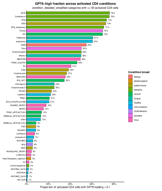
Extended Data Fig. 3d. Bar plot showing the percentage of GP79-active cells among all activated CD4+ T cells across immunological challenges.
(e) Per-cell log2FC heatmap
# ============================================================
# s3e: Per-cell log2FC heatmap of activation GPs (activated cells only),
#      relative to each cell's own-lineage resting baseline
# ============================================================
L <- L_pm_filtered[c(CD4_cells, CD8_cells), GPs_of_interest, drop = FALSE]
cell_ids <- rownames(L)
cell_type <- seurat_meta_filtered$annotation_level2[match(cell_ids, seurat_meta_filtered$cellID)]

set.seed(123)
total_budget <- 8000
small_keep_all <- 150
min_per_cluster <- 150
max_per_cluster <- 600
cells_by_ct <- split(cell_ids, cell_type)
sizes <- sapply(cells_by_ct, length)
alloc <- ifelse(sizes <= small_keep_all, sizes, pmin(min_per_cluster, sizes))
remaining <- total_budget - sum(alloc)
if (remaining > 0) {
  room <- pmax(pmin(sizes, max_per_cluster) - alloc, 0)
  if (sum(room) > 0) {
    extra <- floor(remaining * room / sum(room))
    alloc <- alloc + extra
    leftover <- total_budget - sum(alloc)
    if (leftover > 0) {
      idx <- order(room, decreasing = TRUE)
      for (j in idx) {
        if (leftover <= 0) break
        addable <- pmin(room[j] - extra[j], leftover)
        if (addable > 0) {
          alloc[j] <- alloc[j] + addable
          leftover <- leftover - addable
        }
      }
    }
  }
}
sampled_cells <- unlist(mapply(function(v, m) if (length(v) <= m) v else sample(v, m), cells_by_ct, pmin(alloc, sizes), SIMPLIFY = FALSE), use.names = FALSE)

cell_group_s <- seurat_meta_filtered$annotation_level2_group[match(sampled_cells, seurat_meta_filtered$cellID)]
cell_level2_s <- seurat_meta_filtered$annotation_level2[match(sampled_cells, seurat_meta_filtered$cellID)]
cell_group_s <- trimws(tolower(as.character(cell_group_s)))
cell_level2_s <- trimws(as.character(cell_level2_s))
cell_level1_s <- sapply(strsplit(cell_level2_s, "[_.]"), `[`, 1)
is_w_cell <- grepl("\\.w", cell_level2_s)
valid_idx <- which(!is.na(cell_level2_s) & !tolower(cell_level2_s) %in% c("", "na", "nan") & cell_group_s %in% c("resting", "activated") & !is_w_cell)
final_cells <- sampled_cells[valid_idx]
final_group <- cell_group_s[valid_idx]
final_level1 <- cell_level1_s[valid_idx]
final_level2 <- cell_level2_s[valid_idx]
col_order <- order(final_group, final_level1, final_level2)
final_cells <- final_cells[col_order]
final_group <- final_group[col_order]
final_level1 <- final_level1[col_order]
final_level2 <- final_level2[col_order]

pc <- 1e-10
cap <- 2
group_counts <- sapply(
  list(
    c("GP56", "GP162", "GP36", "GP152", "GP161", "GP177", "GP79", "GP12", "GP13", "GP159"),
    c("GP10", "GP58", "GP181", "GP176"),
    c("GP25", "GP26", "GP35", "GP32", "GP80", "GP57"),
    c("GP9", "GP171", "GP49", "GP41", "GP11")
  ),
  function(gp_group) sum(ordered_GPs %in% gp_group)
)
group_counts <- group_counts[group_counts > 0]
gaps_row <- cumsum(group_counts)[-length(group_counts)]

act_idx <- which(final_group == "activated")
act_cells <- final_cells[act_idx]
act_level1 <- final_level1[act_idx]
act_level2 <- final_level2[act_idx]
act_order <- order(act_level1, act_level2)
act_cells <- act_cells[act_order]
act_level1 <- act_level1[act_order]
act_level2 <- act_level2[act_order]

L_sub_act <- L[act_cells, , drop = FALSE]
M_raw_act <- t(L_sub_act)

# Per-lineage resting baseline: each activated cell's log2FC is computed
# against the mean loading in resting cells of its own lineage.
mu_resting_CD4 <- colMeans(L_pm_filtered[CD4_resting_cells, GPs_of_interest, drop = FALSE])
mu_resting_CD8 <- colMeans(L_pm_filtered[CD8_resting_cells, GPs_of_interest, drop = FALSE])
baseline_mat <- matrix(NA_real_, nrow = nrow(M_raw_act), ncol = ncol(M_raw_act))
rownames(baseline_mat) <- rownames(M_raw_act)
baseline_mat[, act_level1 == "CD4"] <- mu_resting_CD4[rownames(M_raw_act)]
baseline_mat[, act_level1 == "CD8"] <- mu_resting_CD8[rownames(M_raw_act)]
M_fc_act <- log2((M_raw_act + pc) / (baseline_mat + pc))
M_fc_act_cap <- pmax(pmin(M_fc_act, cap), -cap)
M_fc_act_cap <- M_fc_act_cap[ordered_GPs, , drop = FALSE]

ann_col_act <- data.frame(Level2 = factor(act_level2), Level1 = factor(act_level1))
rownames(ann_col_act) <- colnames(M_fc_act_cap)
present_level1_act <- levels(ann_col_act$Level1)
present_level2_act <- levels(ann_col_act$Level2)
level1_cols_act <- ZemmourLib::immgent_colors$level1
level1_cols_act <- level1_cols_act[names(level1_cols_act) %in% present_level1_act]
level2_cols_act <- ZemmourLib::immgent_colors$level2
level2_cols_act <- level2_cols_act[names(level2_cols_act) %in% present_level2_act]
missing_l2_act <- setdiff(present_level2_act, names(level2_cols_act))
if (length(missing_l2_act) > 0) {
  level2_cols_act <- c(level2_cols_act, setNames(rep("grey80", length(missing_l2_act)), missing_l2_act))
}
ann_colors_act <- list(Level1 = level1_cols_act, Level2 = level2_cols_act)

rle_l1_act <- rle(as.character(ann_col_act$Level1))
gaps_col_act <- cumsum(rle_l1_act$lengths)
gaps_col_act <- gaps_col_act[-length(gaps_col_act)]

pheatmap(
  M_fc_act_cap,
  cluster_rows = FALSE, cluster_cols = FALSE,
  gaps_row = gaps_row, gaps_col = gaps_col_act,
  color = colorRampPalette(c("#7A0177", "black", "#FFD700"))(101),
  breaks = seq(-cap, cap, length.out = 102),
  show_colnames = FALSE, fontsize_row = 7, fontface_row = "bold", border_color = NA,
  annotation_col = ann_col_act, annotation_colors = ann_colors_act, annotation_names_col = TRUE,
  useRaster = TRUE,
  main = "GP Log2FC vs per-lineage RESTING baseline (CD4 cells vs CD4 resting; CD8 vs CD8 resting)",
  filename = paste0(figure_path, "s3e.pdf"),
  width = 12, height = 4
)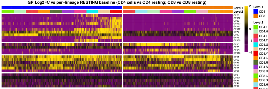
Extended Data Fig. 3e. Heatmap showing single-cell GP activity in activated CD4+ and CD8+ T cells (log2 fold change in GP activity relative to the resting baseline of the same lineage). Cells are grouped by cluster.
(f) GP57+ rate, cancer vs. other conditions
# ============================================================
# s3f: GP57 high-loading proportion, cancer vs other conditions
#      (activated CD4 and CD8)
# ============================================================
gp57_condition_df <- data.frame(
  lineage = seurat_meta_filtered$annotation_level1,
  activation_group = seurat_meta_filtered$annotation_level2_group,
  condition_broad = as.character(seurat_meta_filtered$condition_broad),
  gp57_loading = L_pm_filtered[, "GP57"],
  stringsAsFactors = FALSE
) %>%
  filter(lineage %in% c("CD8", "CD4"), activation_group == "activated") %>%
  mutate(
    lineage = factor(lineage, levels = c("CD8", "CD4")),
    condition_group = if_else(condition_broad == "cancer", "Cancer", "Other conditions"),
    condition_group = factor(condition_group, levels = c("Cancer", "Other conditions")),
    gp57_high = gp57_loading > 0.1
  )

gp57_condition_summary <- gp57_condition_df %>%
  group_by(lineage, condition_group) %>%
  summarise(n_cells = n(), n_gp57_high = sum(gp57_high), proportion_gp57_high = mean(gp57_high), .groups = "drop")

gp57_ymax <- max(gp57_condition_summary$proportion_gp57_high, na.rm = TRUE)
gp57_ymax <- ifelse(gp57_ymax > 0, gp57_ymax * 1.25, 0.05)

p_s3f <- ggplot(gp57_condition_summary, aes(x = lineage, y = proportion_gp57_high, fill = condition_group)) +
  geom_col(position = position_dodge(width = 0.72), width = 0.62, color = "grey20", linewidth = 0.25) +
  geom_text(
    aes(label = paste0(scales::percent(proportion_gp57_high, accuracy = 0.1), "\n", n_gp57_high, "/", n_cells)),
    position = position_dodge(width = 0.72), vjust = -0.25, size = 3.4, lineheight = 0.9
  ) +
  scale_y_continuous(labels = scales::percent_format(accuracy = 1), limits = c(0, gp57_ymax), expand = expansion(mult = c(0, 0.04))) +
  scale_fill_manual(values = c("Cancer" = "#C44E52", "Other conditions" = "#4C72B0")) +
  labs(x = NULL, y = "Proportion of activated cells", fill = "Condition", title = "GP57 loading > 0.1 in activated CD8 and CD4 cells") +
  theme_classic(base_size = 12) +
  theme(legend.position = "top", legend.title = element_text(face = "bold"), axis.text.x = element_text(face = "bold"), plot.title = element_text(face = "bold", hjust = 0.5))
ggsave(filename = paste0(figure_path, "s3f.pdf"), plot = p_s3f, width = 5.4, height = 4.2)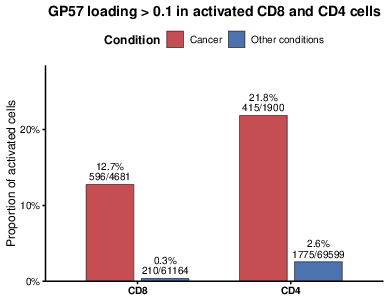
Extended Data Fig. 3f. Bar plot showing the percentage of GP57-active cells among activated CD8+ and CD4+ T cells in cancer versus all other conditions.
sessionInfo()R version 4.5.1 (2025-06-13)
Platform: aarch64-apple-darwin20
Running under: macOS Sequoia 15.6.1
Matrix products: default
BLAS: /System/Library/Frameworks/Accelerate.framework/Versions/A/Frameworks/vecLib.framework/Versions/A/libBLAS.dylib
LAPACK: /Library/Frameworks/R.framework/Versions/4.5-arm64/Resources/lib/libRlapack.dylib; LAPACK version 3.12.1
locale:
[1] en_CA/en_CA/en_CA/C/en_CA/en_CA
time zone: America/Chicago
tzcode source: internal
attached base packages:
[1] stats graphics grDevices utils datasets methods base
loaded via a namespace (and not attached):
[1] vctrs_0.7.3 cli_3.6.6 knitr_1.50 rlang_1.2.0
[5] xfun_0.55 stringi_1.8.9 otel_0.2.0 promises_1.5.0
[9] jsonlite_2.0.0 workflowr_1.7.2 glue_1.8.1 rprojroot_2.1.1
[13] git2r_0.36.2 htmltools_0.5.9 httpuv_1.6.16 sass_0.4.10
[17] rmarkdown_2.30 evaluate_1.0.5 jquerylib_0.1.4 tibble_3.3.0
[21] fastmap_1.2.0 yaml_2.3.12 lifecycle_1.0.5 whisker_0.4.1
[25] stringr_1.6.0 compiler_4.5.1 fs_1.6.6 Rcpp_1.1.1-1.1
[29] pkgconfig_2.0.3 later_1.4.4 digest_0.6.39 R6_2.6.1
[33] pillar_1.11.1 magrittr_2.0.5 bslib_0.9.0 tools_4.5.1
[37] cachem_1.1.0