Getting Started: Fitting sGP to a Synthetic Dataset
Ziang Zhang
2024-11-20
Last updated: 2024-11-21
Checks: 7 0
Knit directory: online_tut/
This reproducible R Markdown analysis was created with workflowr (version 1.7.1). The Checks tab describes the reproducibility checks that were applied when the results were created. The Past versions tab lists the development history.
Great! Since the R Markdown file has been committed to the Git repository, you know the exact version of the code that produced these results.
Great job! The global environment was empty. Objects defined in the global environment can affect the analysis in your R Markdown file in unknown ways. For reproduciblity it’s best to always run the code in an empty environment.
The command set.seed(20241120) was run prior to running
the code in the R Markdown file. Setting a seed ensures that any results
that rely on randomness, e.g. subsampling or permutations, are
reproducible.
Great job! Recording the operating system, R version, and package versions is critical for reproducibility.
Nice! There were no cached chunks for this analysis, so you can be confident that you successfully produced the results during this run.
Great job! Using relative paths to the files within your workflowr project makes it easier to run your code on other machines.
Great! You are using Git for version control. Tracking code development and connecting the code version to the results is critical for reproducibility.
The results in this page were generated with repository version 7878a82. See the Past versions tab to see a history of the changes made to the R Markdown and HTML files.
Note that you need to be careful to ensure that all relevant files for
the analysis have been committed to Git prior to generating the results
(you can use wflow_publish or
wflow_git_commit). workflowr only checks the R Markdown
file, but you know if there are other scripts or data files that it
depends on. Below is the status of the Git repository when the results
were generated:
Ignored files:
    Ignored:    .DS_Store
    Ignored:    .Rproj.user/
    Ignored:    analysis/.DS_Store
    Ignored:    code/.DS_Store

Untracked files:
    Untracked:  code/functions.R
    Untracked:  code/tut.cpp
    Untracked:  code/tut.o
    Untracked:  code/tut.so

Unstaged changes:
    Modified:   analysis/_site.yml
    Deleted:    analysis/license.Rmd
    Modified:   analysis/lynx.rmd
Note that any generated files, e.g. HTML, png, CSS, etc., are not included in this status report because it is ok for generated content to have uncommitted changes.
These are the previous versions of the repository in which changes were
made to the R Markdown (analysis/starter.rmd) and HTML
(docs/starter.html) files. If you’ve configured a remote
Git repository (see ?wflow_git_remote), click on the
hyperlinks in the table below to view the files as they were in that
past version.
| File | Version | Author | Date | Message |
|---|---|---|---|---|
| html | 96b32c6 | Ziang Zhang | 2024-11-21 | Build site. |
| Rmd | 1a0cfcb | Ziang Zhang | 2024-11-21 | workflowr::wflow_publish("analysis/starter.rmd") |
| html | c4bd829 | Ziang Zhang | 2024-11-21 | Build site. |
| Rmd | 7fb7a81 | Ziang Zhang | 2024-11-21 | workflowr::wflow_publish("analysis/starter.rmd") |
library(BayesGP)
library(tidyverse)
library(parallel)
source("code/functions.R")
Introduction
In this tutorial, we introduce the basic steps to fit a sGP model using the seasonal B-spline approximation introduced in Zhang et al, 2024.
For illustration, we use one of the synthetic datasets described in the main paper. The dataset and its corresponding true function are shown in the plots below.
n <- 500
location_of_interest <- seq(0, 10, length.out = 500)
true_f <- function(x){
  if(x < 2){
    return(2*sin(2 * 2 * pi * x) * (3-x))
  } else if (x > 2 && x < 4){
    return(2*sin(2 * 2 * pi * x))
  } else{
    return(2*sin(2 * 2 * pi * x) * (log(x-3) + 1))
  }
}
true_f <- Vectorize(true_f)

set.seed(123)
data <- simulate_data_poisson(func = true_f, n = n, sigma = 0.5, region = c(0,10), offset = 0)

par(mfrow = c(1,2))
plot(data$x, data$y, type = "p", col = "black",
     pch = 20, cex = 0.5,
     ylab = "y", xlab = "x")
lines(location_of_interest, exp(true_f(location_of_interest)), col = "red", lwd = 2)
plot(location_of_interest, true_f(location_of_interest),
     type = "l", col = "black",
     pch = 20, cex = 0.5,
     ylab = "y", xlab = "x")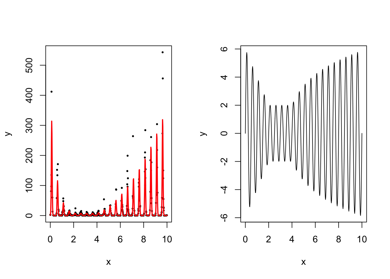
| Version | Author | Date |
|---|---|---|
| c4bd829 | Ziang Zhang | 2024-11-21 |
par(mfrow = c(1,1))The hierarchical model we consider is as follows:
\[\begin{equation} \begin{aligned} Y_i|x_i,\xi_i &\sim \text{Poisson}(\lambda_i), \\ \text{log}(\lambda_i) &= g(x_i) + \xi_i, \\ g(x) &\sim \text{sGP}(\sigma_x), \\ \xi_i &\sim \text{N}(0, \sigma_\xi^2). \end{aligned} \end{equation}\]
We assume the sGP prior has a frequency of \(2\) (\(\alpha = 4\pi\)), and use an Exponential prior for the one-step PSD \(\sigma_x(1)\) defined as: \[ \text{P}(\sigma_x(1) > 2) = 0.1. \]
The standard deviation \(\sigma_\xi\) of the observation-level random intercept follows an Exponential prior with a median of \(1\).
To make the computation more efficient, we will use \(10\) equally spaced knots to define the B-spline basis, which will then be used to approximate the sGP prior.
Inference
To make approximate Bayesian inference of the above model, we make
use of the BayesGP package:
mod <- BayesGP::model_fit(
    y ~ f(
      x,
      model = "sgp",
      region = c(0,10),
      freq = 2,
      k = 10, # number of knots
      sd.prior = list(param = list(u = 2, alpha = 0.1), h = 1)
    ) +
      f(index, model = "iid", sd.prior = 1),
    data = data,
    family = "Poisson"
  )
We can take a quick look at the posterior summary:
summary(mod)Here are some posterior/prior summaries for the parameters:
name median q0.025 q0.975 prior prior:P1 prior:P2
1 intercept 0.106 -0.055 0.274 Normal 0 1e+03
2 x (PSD) 0.890 0.636 1.342 Exponential 2 1e-01
3 index (SD) 0.485 0.423 0.556 Exponential 1 5e-01
For Normal prior, P1 is its mean and P2 is its variance.
For Exponential prior, prior is specified as P(theta > P1) = P2. We can also obtain the posterior of \(g\) at any location of interest:
post_g <- predict(mod, newdata = data.frame(x = location_of_interest), variable = "x")
head(post_g)
x q0.025 q0.5 q0.975 mean
1 0.00000000 -0.1867575 0.2723952 0.711317 0.2688137
2 0.02004008 1.2278211 1.6493109 2.052013 1.6462239
3 0.04008016 2.5478229 2.9261264 3.291498 2.9251860
4 0.06012024 3.6668587 4.0243567 4.373277 4.0238335
5 0.08016032 4.5179810 4.8739401 5.217268 4.8721472
6 0.10020040 5.0675664 5.4185435 5.772141 5.4165004Take a look at the plot of them:
plot(location_of_interest, true_f(location_of_interest),
     type = "l", col = "black",
     pch = 20, cex = 0.5,
     ylab = "y", xlab = "x")
lines(x = location_of_interest, y = (post_g$mean), col = "blue", lwd = 1, lty = 2)
polygon(c(location_of_interest, rev(location_of_interest)),
        c(post_g$q0.025, rev(post_g$q0.975)),
        col = adjustcolor("blue", alpha.f = 0.2), border = NA)
legend("topright", legend = c("True function", "Posterior mean"),
       col = c("black", "blue"), lty = c(1, 2), lwd = c(1, 1))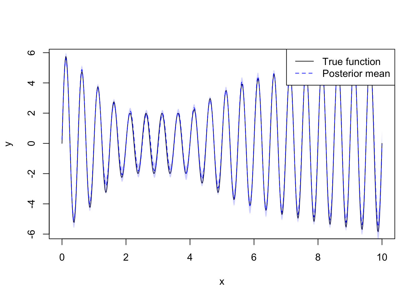
| Version | Author | Date |
|---|---|---|
| c4bd829 | Ziang Zhang | 2024-11-21 |
We can also just obtain the raw samples of \(g\) at these locations:
post_g_raw <- predict(mod, newdata = data.frame(x = location_of_interest), variable = "x", only.samples = TRUE)
plot(location_of_interest, true_f(location_of_interest),
     type = "l", col = "black",
     pch = 20, cex = 0.5,
     ylab = "y", xlab = "x")
matlines(location_of_interest, post_g_raw[,2:12], col = "pink", lty = 2, lwd = 0.5)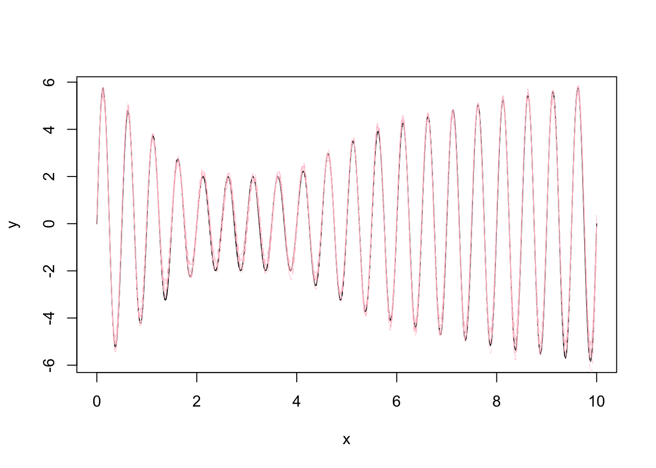
| Version | Author | Date |
|---|---|---|
| c4bd829 | Ziang Zhang | 2024-11-21 |
sessionInfo()R version 4.3.1 (2023-06-16)
Platform: aarch64-apple-darwin20 (64-bit)
Running under: macOS Monterey 12.7.4
Matrix products: default
BLAS: /Library/Frameworks/R.framework/Versions/4.3-arm64/Resources/lib/libRblas.0.dylib
LAPACK: /Library/Frameworks/R.framework/Versions/4.3-arm64/Resources/lib/libRlapack.dylib; LAPACK version 3.11.0
locale:
[1] en_US.UTF-8/en_US.UTF-8/en_US.UTF-8/C/en_US.UTF-8/en_US.UTF-8
time zone: America/Chicago
tzcode source: internal
attached base packages:
[1] parallel stats graphics grDevices utils datasets methods
[8] base
other attached packages:
[1] lubridate_1.9.3 forcats_1.0.0 stringr_1.5.1 dplyr_1.1.4
[5] purrr_1.0.2 readr_2.1.5 tidyr_1.3.1 tibble_3.2.1
[9] ggplot2_3.5.1 tidyverse_2.0.0 BayesGP_0.1.3 workflowr_1.7.1
loaded via a namespace (and not attached):
[1] gtable_0.3.6 TMB_1.9.15 xfun_0.48
[4] bslib_0.8.0 ks_1.14.3 processx_3.8.4
[7] lattice_0.22-6 numDeriv_2016.8-1.1 callr_3.7.6
[10] tzdb_0.4.0 bitops_1.0-9 vctrs_0.6.5
[13] tools_4.3.1 ps_1.8.0 generics_0.1.3
[16] aghq_0.4.1 fansi_1.0.6 cluster_2.1.6
[19] highr_0.11 pkgconfig_2.0.3 fds_1.8
[22] KernSmooth_2.23-24 Matrix_1.6-4 data.table_1.16.2
[25] lifecycle_1.0.4 compiler_4.3.1 git2r_0.33.0
[28] statmod_1.5.0 munsell_0.5.1 getPass_0.2-4
[31] mvQuad_1.0-8 httpuv_1.6.15 htmltools_0.5.8.1
[34] rainbow_3.8 sass_0.4.9 RCurl_1.98-1.16
[37] yaml_2.3.10 pracma_2.4.4 later_1.3.2
[40] pillar_1.9.0 jquerylib_0.1.4 whisker_0.4.1
[43] MASS_7.3-60 cachem_1.1.0 mclust_6.1.1
[46] tidyselect_1.2.1 digest_0.6.37 mvtnorm_1.3-1
[49] stringi_1.8.4 splines_4.3.1 pcaPP_2.0-5
[52] rprojroot_2.0.4 fastmap_1.2.0 grid_4.3.1
[55] colorspace_2.1-1 cli_3.6.3 magrittr_2.0.3
[58] utf8_1.2.4 withr_3.0.2 scales_1.3.0
[61] promises_1.3.0 timechange_0.3.0 rmarkdown_2.28
[64] httr_1.4.7 deSolve_1.40 hms_1.1.3
[67] evaluate_1.0.1 knitr_1.48 rlang_1.1.4
[70] Rcpp_1.0.13-1 hdrcde_3.4 glue_1.8.0
[73] fda_6.2.0 rstudioapi_0.16.0 jsonlite_1.8.9
[76] R6_2.5.1 fs_1.6.4