Pseudotime analysis with slingshot
Lambda Moses
2019-08-15
Last updated: 2019-08-15
Checks: 7 0
Knit directory: BUS_notebooks_R/
This reproducible R Markdown analysis was created with workflowr (version 1.4.0). The Checks tab describes the reproducibility checks that were applied when the results were created. The Past versions tab lists the development history.
Great! Since the R Markdown file has been committed to the Git repository, you know the exact version of the code that produced these results.
Great job! The global environment was empty. Objects defined in the global environment can affect the analysis in your R Markdown file in unknown ways. For reproduciblity it’s best to always run the code in an empty environment.
The command set.seed(20181214) was run prior to running the code in the R Markdown file. Setting a seed ensures that any results that rely on randomness, e.g. subsampling or permutations, are reproducible.
Great job! Recording the operating system, R version, and package versions is critical for reproducibility.
Nice! There were no cached chunks for this analysis, so you can be confident that you successfully produced the results during this run.
Great job! Using relative paths to the files within your workflowr project makes it easier to run your code on other machines.
Great! You are using Git for version control. Tracking code development and connecting the code version to the results is critical for reproducibility. The version displayed above was the version of the Git repository at the time these results were generated.
Note that you need to be careful to ensure that all relevant files for the analysis have been committed to Git prior to generating the results (you can use wflow_publish or wflow_git_commit). workflowr only checks the R Markdown file, but you know if there are other scripts or data files that it depends on. Below is the status of the Git repository when the results were generated:
Ignored files:
    Ignored:    .Rhistory
    Ignored:    .Rproj.user/
    Ignored:    BUS_notebooks_R.Rproj
    Ignored:    analysis/figure/
    Ignored:    data/whitelist_v3.txt.gz
    Ignored:    output/out_pbmc1k/

Untracked files:
    Untracked:  ensembl/
    Untracked:  output/neuron10k/
Note that any generated files, e.g. HTML, png, CSS, etc., are not included in this status report because it is ok for generated content to have uncommitted changes.
These are the previous versions of the R Markdown and HTML files. If you’ve configured a remote Git repository (see ?wflow_git_remote), click on the hyperlinks in the table below to view them.
| File | Version | Author | Date | Message |
|---|---|---|---|---|
| Rmd | b6cf111 | Lambda Moses | 2019-08-15 | Updated for new version of parsnip, and rebuilt with Ensembl 97 |
| Rmd | 834b100 | Lambda Moses | 2019-08-13 | Merge branch ‘master’ of https://github.com/BUStools/BUS_notebooks_R |
| Rmd | 1fee539 | Lambda Moses | 2019-08-13 | Added mode argument to rand_forest |
| Rmd | f8a015a | Lior Pachter | 2019-07-26 | Update slingshot.Rmd |
| html | ababa88 | Lambda Moses | 2019-07-25 | Build site. |
| Rmd | 7c215a4 | Lambda Moses | 2019-07-25 | Just realized that the Leiden clustering is not reproducible. Installed Seurat |
| html | 906799e | Lambda Moses | 2019-07-24 | Build site. |
| Rmd | 63e0c03 | Lambda Moses | 2019-07-24 | slingshot notebook |
| html | df34d05 | Lambda Moses | 2019-07-24 | Build site. |
| Rmd | 5e16aa3 | Lambda Moses | 2019-07-24 | slingshot notebook |
Introduction
This notebook does pseudotime analysis of the 10x 10k neurons from an E18 mouse using slingshot, which is on Bioconductor. The notebook begins with pre-processing of the reads with the kallisto | bustools workflow Like Monocle 2 DDRTree, slingshot builds a minimum spanning tree, but while Monocle 2 builds the tree from individual cells, slingshot does so with clusters. slingshot is also the top rated trajectory inference method in the dynverse paper.
In the kallisto | bustools paper, I used the docker container for slingshot provided by dynverse for pseudotime analysis, because dynverse provides unified interface to dozens of different trajectory inference (TI) methods via docker containers, making it easy to try other methods without worrying about installing dependencies. Furthermore, dynverse provides metrics to evaluate TI methods. However, the docker images provided by dynverse do not provide users with the full range of options available from the TI methods themselves. For instance, while any dimension reduction and any kind of clustering can be used for slingshot, dynverse chose PCA and partition around medoids (PAM) clustering for us (see the source code here). So in this notebook, we will directly use slingshot rather than via dynverse.
The gene count matrix of the 10k neuron dataset has already been generated with the kallisto | bustools pipeline and filtered for the Monocle 2 notebook. Cell types have also been annotated with SingleR in that notebook. Please refer to the first 3 main sections of that notebook for instructions on how to use kallisto | bustools, remove empty droplets, and annotate cell types.
Package slingshot is from Bioconductor. BUSpaRse is on GitHub. The other packages are on CRAN.
library(slingshot)
library(BUSpaRse)
library(tidyverse)
library(tidymodels)
library(Seurat)
library(scales)
library(viridis)
library(Matrix)
Loading the matrix
The filtered gene count matrix and the cell annotation were saved from the Monocle 2 notebook.
annot <- readRDS("./output/neuron10k/cell_type.rds")
mat_filtered <- readRDS("./output/neuron10k/mat_filtered.rds")
Just to show the structures of those 2 objects:
dim(mat_filtered)#> [1] 23516 11037class(mat_filtered)#> [1] "dgCMatrix"
#> attr(,"package")
#> [1] "Matrix"Row names are Ensembl gene IDs.
head(rownames(mat_filtered))#> [1] "ENSMUSG00000094619.2" "ENSMUSG00000095646.1" "ENSMUSG00000092401.3"
#> [4] "ENSMUSG00000109389.1" "ENSMUSG00000092212.3" "ENSMUSG00000079293.11"head(colnames(mat_filtered))#> [1] "AAACCCACACGCGGTT" "AAACCCACAGCATACT" "AAACCCACATACCATG"
#> [4] "AAACCCAGTCGCACAC" "AAACCCAGTGCACATT" "AAACCCAGTGGTAATA"str(annot)#> List of 10
#> $ scores : num [1:11037, 1:28] 0.188 0.194 0.182 0.267 0.187 ...
#> ..- attr(*, "dimnames")=List of 2
#> .. ..$ : chr [1:11037] "AAACCCACACGCGGTT" "AAACCCACAGCATACT" "AAACCCACATACCATG" "AAACCCAGTCGCACAC" ...
#> .. ..$ : chr [1:28] "Adipocytes" "aNSCs" "Astrocytes" "Astrocytes activated" ...
#> $ labels : chr [1:11037, 1] "NPCs" "NPCs" "NPCs" "NPCs" ...
#> ..- attr(*, "dimnames")=List of 2
#> .. ..$ : chr [1, 1:11037] "AAACCCACACGCGGTT" "AAACCCACAGCATACT" "AAACCCACATACCATG" "AAACCCAGTCGCACAC" ...
#> .. ..$ : NULL
#> $ r : num [1:11037, 1:358] 0.187 0.197 0.179 0.251 0.171 ...
#> ..- attr(*, "dimnames")=List of 2
#> .. ..$ : chr [1:11037] "AAACCCACACGCGGTT" "AAACCCACAGCATACT" "AAACCCACATACCATG" "AAACCCAGTCGCACAC" ...
#> .. ..$ : chr [1:358] "ERR525589Aligned" "ERR525592Aligned" "SRR275532Aligned" "SRR275534Aligned" ...
#> $ pval : Named num [1:11037] 0.0428 0.058 0.0383 0.0111 0.0327 ...
#> ..- attr(*, "names")= chr [1:11037] "AAACCCACACGCGGTT" "AAACCCACAGCATACT" "AAACCCACATACCATG" "AAACCCAGTCGCACAC" ...
#> $ labels1 : chr [1:11037, 1] "NPCs" "NPCs" "NPCs" "NPCs" ...
#> ..- attr(*, "dimnames")=List of 2
#> .. ..$ : chr [1:11037] "AAACCCACACGCGGTT" "AAACCCACAGCATACT" "AAACCCACATACCATG" "AAACCCAGTCGCACAC" ...
#> .. ..$ : NULL
#> $ labels1.thres: chr [1:11037] "NPCs" "X" "NPCs" "NPCs" ...
#> $ cell.names : chr [1:11037] "AAACCCACACGCGGTT" "AAACCCACAGCATACT" "AAACCCACATACCATG" "AAACCCAGTCGCACAC" ...
#> $ quantile.use : num 0.8
#> $ types : chr [1:358] "Adipocytes" "Adipocytes" "Adipocytes" "Adipocytes" ...
#> $ method : chr "single"To prevent endothelial cells, erythrocytes, immune cells, and fibroblasts from being mistaken as very differentiated cell types derived from neural stem cells, we will only keep cells with a label for the neural or glial lineage. This can be a problem as slingshot does not support multiple disconnected trajectories.
ind <- annot$labels %in% c("NPCs", "Neurons", "OPCs", "Oligodendrocytes",
                           "qNSCs", "aNSCs", "Astrocytes", "Ependymal")
cells_use <- annot$cell.names[ind]
mat_filtered <- mat_filtered[, cells_use]
Meaning of the acronyms:
- NPCs: Neural progenitor cells
- OPCs: Oligodendrocyte progenitor cells
- qNSCs: Quiescent neural stem cells
- aNSCs: Active neural stem cells
Since we will do differential expression and gene symbols are more human readable than Ensembl gene IDs, we will get the corresponding gene symbols from Ensembl.
gns <- tr2g_ensembl(species = "Mus musculus", use_gene_name = TRUE,
                    ensembl_version = 97)[,c("gene", "gene_name")] %>%
  distinct()
#> Querying biomart for transcript and gene IDs of Mus musculus#> Note: requested host was redirected from
#> http://jul2019.archive.ensembl.org to https://www.ensembl.org:443/biomart/martservice#> This often occurs when connecting to the archive URL for the current Ensembl release#> You can check the current version number using listEnsemblArchives()#> Cache foundPreprocessing
QC
seu <- CreateSeuratObject(mat_filtered) %>%
  SCTransform() # normalize and scale
# Add cell type annotation to metadata
seu <- AddMetaData(seu, setNames(annot$labels[ind], cells_use),
                   col.name = "cell_type")
VlnPlot(seu, c("nCount_RNA", "nFeature_RNA"), pt.size = 0.1, ncol = 1, group.by = "cell_type")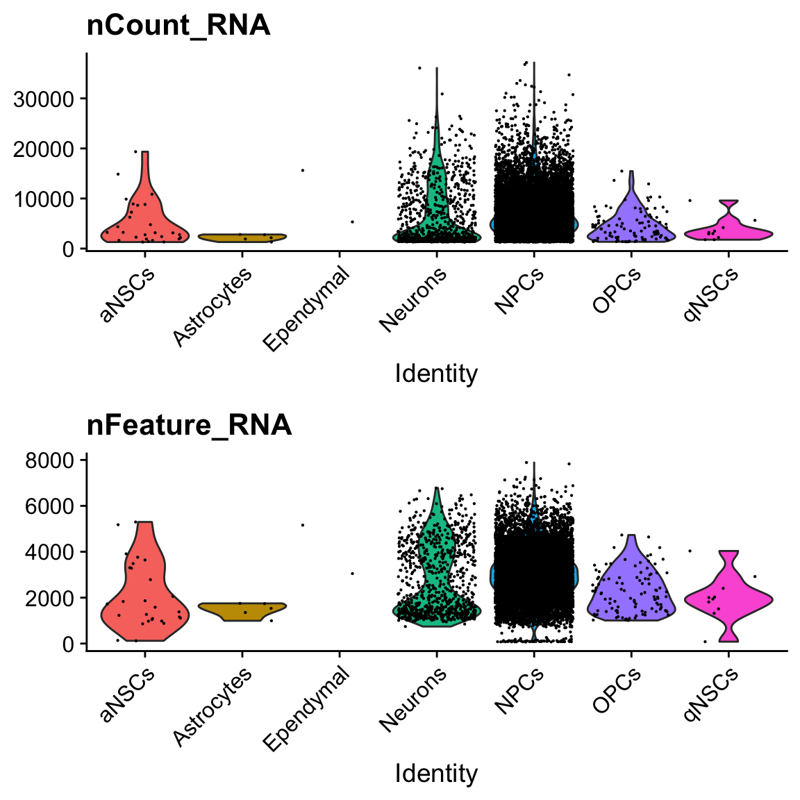
| Version | Author | Date |
|---|---|---|
| df34d05 | Lambda Moses | 2019-07-24 |
There are only 2 cells labeled ependymal.
ggplot(seu@meta.data, aes(nCount_RNA, nFeature_RNA, color = cell_type)) +
  geom_point(size = 0.5) +
  scale_color_brewer(type = "qual", palette = "Set2", name = "cell type") +
  scale_x_log10() +
  scale_y_log10() +
  theme_bw() +
  # Make points larger in legend
  guides(color = guide_legend(override.aes = list(size = 3))) +
  labs(x = "Total UMI counts", y = "Number of genes detected")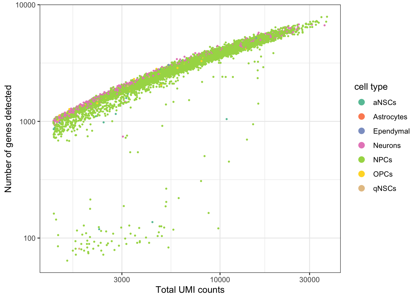
| Version | Author | Date |
|---|---|---|
| df34d05 | Lambda Moses | 2019-07-24 |
Dimension reduction
seu <- RunPCA(seu, npcs = 70, verbose = FALSE)
ElbowPlot(seu, ndims = 70)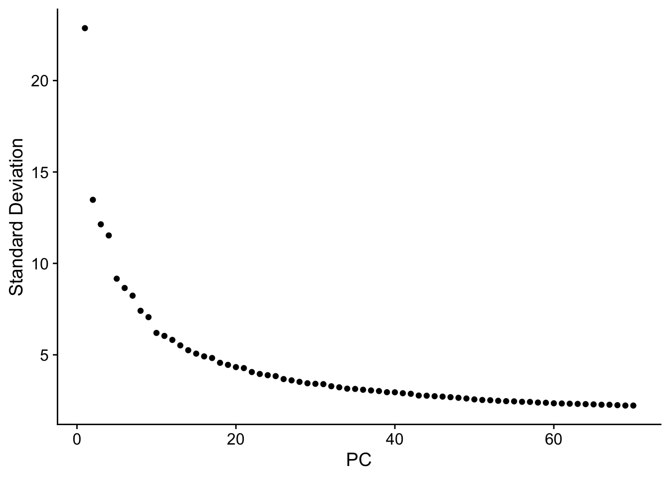
| Version | Author | Date |
|---|---|---|
| df34d05 | Lambda Moses | 2019-07-24 |
The y axis is standard deviation (not variance), or the singular values from singular value decomposition on the data performed for PCA.
# Need to use DimPlot due to weird workflowr problem with PCAPlot that calls seu[[wflow.build]]
# and eats up memory. I suspect this is due to the sys.call() in
# Seurat:::SpecificDimPlot.
DimPlot(seu, reduction = "pca",
        group.by = "cell_type", pt.size = 0.5, label = TRUE, repel = TRUE) +
  scale_color_brewer(type = "qual", palette = "Set2")
#> Warning: Using `as.character()` on a quosure is deprecated as of rlang 0.3.0.
#> Please use `as_label()` or `as_name()` instead.
#> This warning is displayed once per session.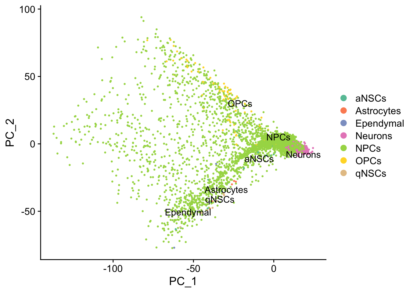
| Version | Author | Date |
|---|---|---|
| df34d05 | Lambda Moses | 2019-07-24 |
seu <- RunTSNE(seu, dims = 1:50, verbose = FALSE)
DimPlot(seu, reduction = "tsne",
        group.by = "cell_type", pt.size = 0.5, label = TRUE, repel = TRUE) +
  scale_color_brewer(type = "qual", palette = "Set2")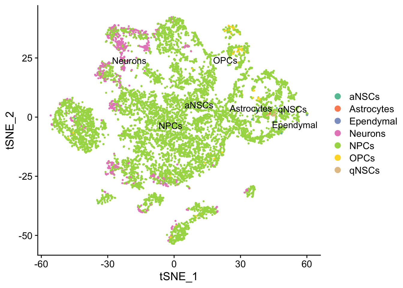
| Version | Author | Date |
|---|---|---|
| df34d05 | Lambda Moses | 2019-07-24 |
UMAP can better preserve pairwise distance of cells than tSNE and can better separate cell populations than the first 2 PCs of PCA (Becht et al. 2018), so the TI will be done on UMAP rather than tSNE or PCA. Note that the messages printed below are from the development version of Seurat (not yet on CRAN). The CRAN version still calls Python UMAP so probably does not work on servers. See the RNA velocity notebook for an example of a work around using uwot.
Idents(seu) <- "cell_type"
DimPlot(seu[, WhichCells(seu, idents = "aNSCs")], reduction = "umap",
        group.by = "cell_type", pt.size = 0.5, label = TRUE, repel = TRUE) +
  scale_color_brewer(type = "qual", palette = "Set2")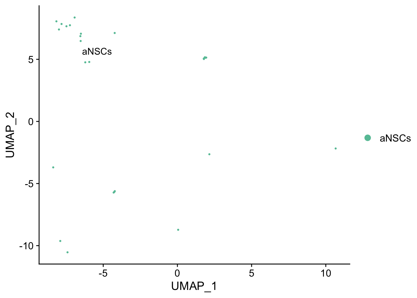
seu <- RunUMAP(seu, dims = 1:50, seed.use = 4867)#> Warning: The default method for RunUMAP has changed from calling Python UMAP via reticulate to the R-native UWOT using the cosine metric
#> To use Python UMAP via reticulate, set umap.method to 'umap-learn' and metric to 'correlation'
#> This message will be shown once per session#> 11:52:58 Read 10699 rows and found 50 numeric columns#> 11:52:58 Using Annoy for neighbor search, n_neighbors = 30#> 11:52:58 Building Annoy index with metric = cosine, n_trees = 50#> 0% 10 20 30 40 50 60 70 80 90 100%#> [----|----|----|----|----|----|----|----|----|----|#> **************************************************|
#> 11:53:00 Writing NN index file to temp file /var/folders/tg/cv0dwcv11q5g13yjt9mc_nh00000gn/T//RtmpzFVtTZ/file4d6b4a23cbc5
#> 11:53:00 Searching Annoy index using 1 thread, search_k = 3000
#> 11:53:03 Annoy recall = 100%
#> 11:53:04 Commencing smooth kNN distance calibration using 1 thread
#> 11:53:05 Initializing from normalized Laplacian + noise
#> 11:53:06 Commencing optimization for 200 epochs, with 430906 positive edges
#> 11:53:13 Optimization finishedDimPlot(seu, reduction = "umap",
group.by = "cell_type", pt.size = 0.5, label = TRUE, repel = TRUE) +
scale_color_brewer(type = "qual", palette = "Set2")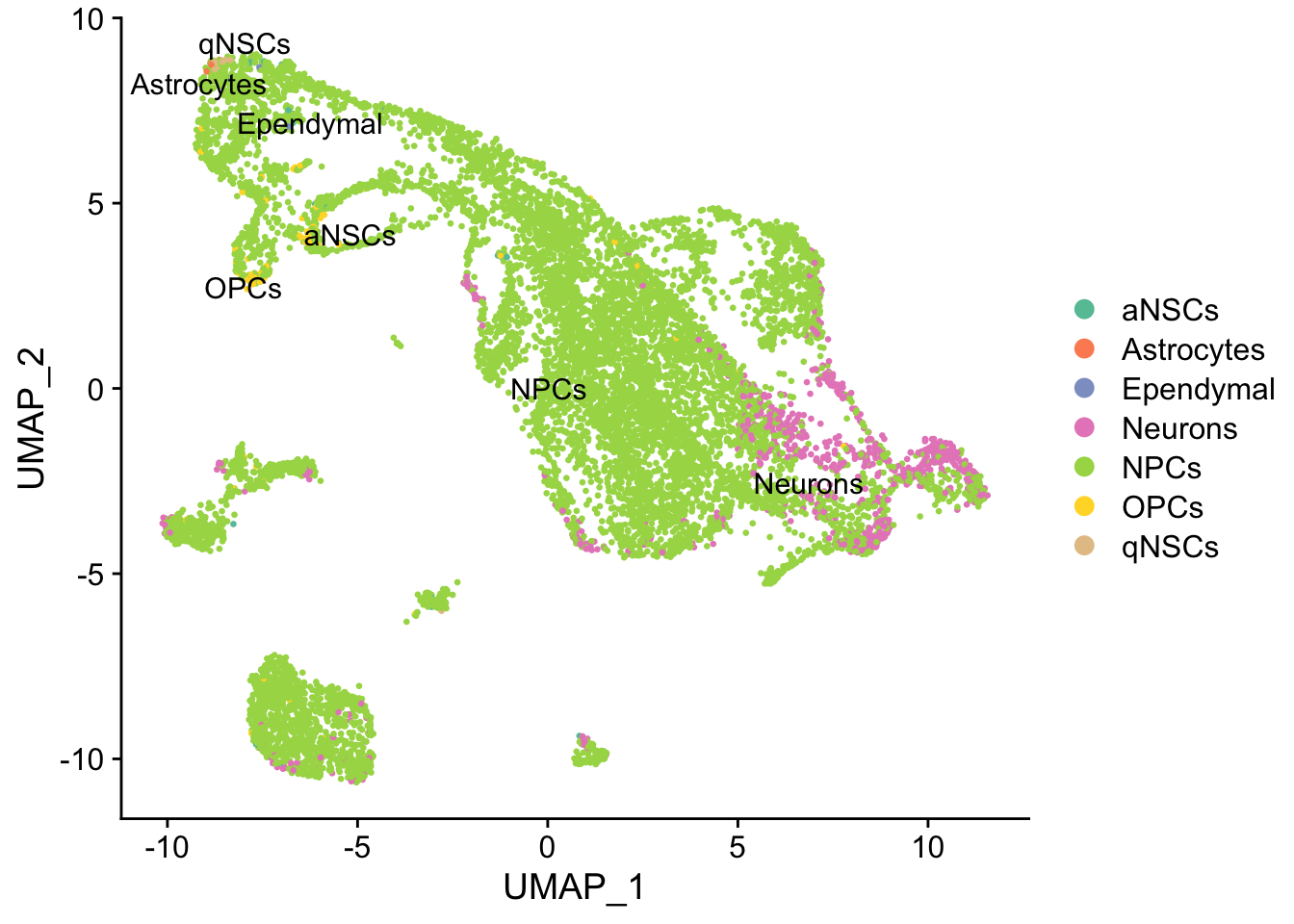
| Version | Author | Date |
|---|---|---|
| df34d05 | Lambda Moses | 2019-07-24 |
Cell type annotation with SingleR requires a reference with bulk RNA seq data for isolated known cell types. The reference used for cell type annotation here does not differentiate between different types of neural progenitor cells; clustering can further partition the neural progenitor cells. Furthermore, slingshot is based on cluster-wise minimum spanning tree, so finding a good clustering is important to good trajectory inference with slingshot. The clustering algorithm used here is Leiden, which is an improvement over the commonly used Louvain; Leiden communities are guaranteed to be well-connected, while Louvain can lead to poorly connected communities.
names(seu@meta.data)#> [1] "orig.ident" "nCount_RNA" "nFeature_RNA"
#> [4] "nCount_SCT" "nFeature_SCT" "cell_type"
#> [7] "SCT_snn_res.1" "seurat_clusters" "SCT_snn_res.0.8"
#> [10] "SCT_snn_res.0.7" "SCT_snn_res.0.6"seu <- FindNeighbors(seu, verbose = FALSE, dims = 1:50)
seu <- FindClusters(seu, algorithm = 4, random.seed = 256, resolution = 1)
DimPlot(seu, pt.size = 0.5, reduction = "umap", group.by = "seurat_clusters", label = TRUE)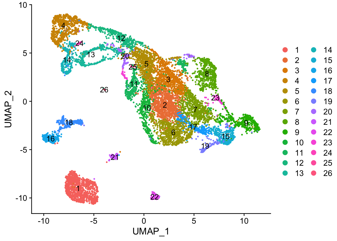
Note that in the current CRAN release of Seurat, Leiden clustering does not take the random seed and gives a somewhat different result every time it’s run. To make the random seed take effect, install the development version of Seurat.
Slingshot
Trajectory inference
While the slingshot vignette uses SingleCellExperiment, slingshot can also take a matrix of cell embeddings in reduced dimension as input. We can optionally specify the cluster to start or end the trajectory based on biological knowledge. Here, since quiescent neural stem cells are in cluster 4, the starting cluster would be 4 near the top left of the previous plot.
sds <- slingshot(Embeddings(seu, "umap"), clusterLabels = seu$seurat_clusters,
                 start.clus = 4, stretch = 0)
Unfortunately, slingshot does not natively support ggplot2. So this is a function that assigns colors to each cell in base R graphics.
#' Assign a color to each cell based on some value
#'
#' @param cell_vars Vector indicating the value of a variable associated with cells.
#' @param pal_fun Palette function that returns a vector of hex colors, whose
#' argument is the length of such a vector.
#' @param ... Extra arguments for pal_fun.
#' @return A vector of hex colors with one entry for each cell.
cell_pal <- function(cell_vars, pal_fun,...) {
  if (is.numeric(cell_vars)) {
    pal <- pal_fun(100, ...)
    return(pal[cut(cell_vars, breaks = 100)])
  } else {
    categories <- sort(unique(cell_vars))
    pal <- setNames(pal_fun(length(categories), ...), categories)
    return(pal[cell_vars])
  }
}
We need color palettes for both cell types and Leiden clusters. These would be the same colors seen in the Seurat plots.
cell_colors <- cell_pal(seu$cell_type, brewer_pal("qual", "Set2"))
cell_colors_clust <- cell_pal(seu$seurat_clusters, hue_pal())
What does the inferred trajectory look like compared to cell types?
plot(reducedDim(sds), col = cell_colors, pch = 16, cex = 0.5)
lines(sds, lwd = 2, type = 'lineages', col = 'black')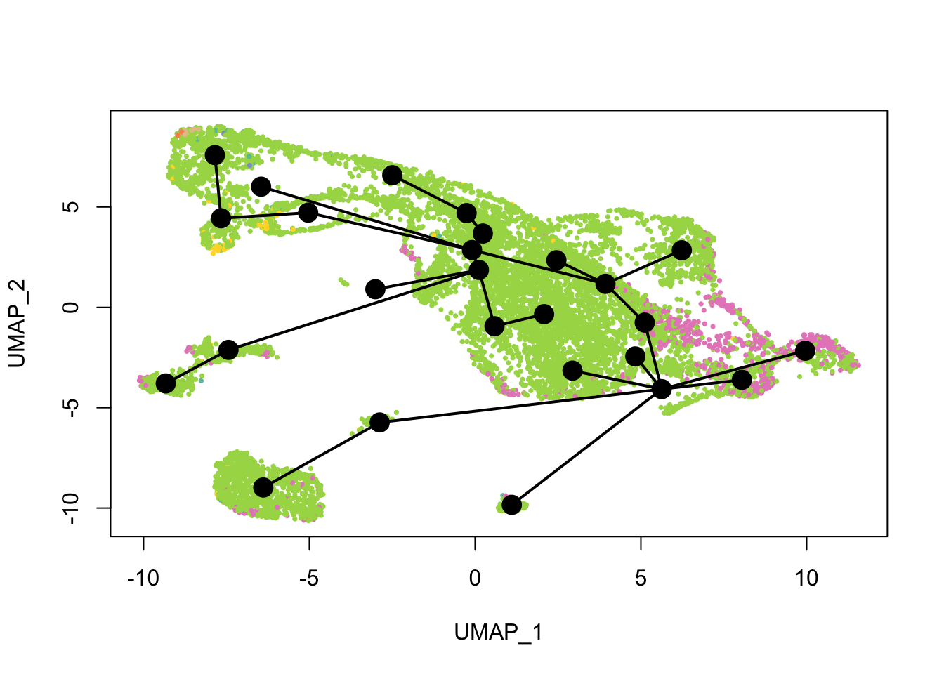
Again, the qNSCs are the brown points near the top left, NPCs are green, and neurons are pink. It seems that multiple neural lineages formed. This is a much more complicated picture than the two branches of neurons projected on the first two PCs in the pseudotime figure in the kallisto | bustools paper (Supplementary Figure 6.5). It also seems that slingshot did not pick up the glial lineage (oligodendrocytes and astrocytes), as the vast majority of cells here are NPCs or neurons.
See how this looks with Leiden clusters.
plot(reducedDim(sds), col = cell_colors_clust, pch = 16, cex = 0.5)
lines(sds, lwd = 2, type = 'lineages', col = 'black')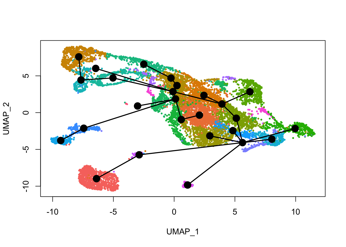
Here slingshot thinks that somewhere around cluster 6 is a point where multiple neural lineages diverge. Different clustering (e.g. different random initiations of Louvain or Leiden algorithms) can lead to somewhat different trajectories, the the main structure is not affected. With different runs of Leiden clustering (without fixed seed), the branching point is placed in the region around its current location, near the small UMAP offshoot there.
Principal curves are smoothed representations of each lineage; pseudotime values are computed by projecting the cells onto the principal curves. What do the principal curves look like?
plot(reducedDim(sds), col = cell_colors, pch = 16, cex = 0.5)
lines(sds, lwd = 2, col = 'black')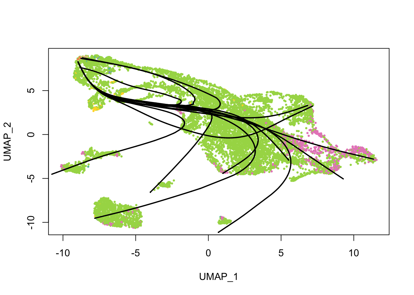
Which cells are in which lineage? Here we plot the pseudotime values for each lineage.
nc <- 3
pt <- slingPseudotime(sds)
nms <- colnames(pt)
nr <- ceiling(length(nms)/nc)
pal <- viridis(100, end = 0.95)
par(mfrow = c(nr, nc))
for (i in nms) {
  colors <- pal[cut(pt[,i], breaks = 100)]
  plot(reducedDim(sds), col = colors, pch = 16, cex = 0.5, main = i)
  lines(sds, lwd = 2, col = 'black', type = 'lineages')
}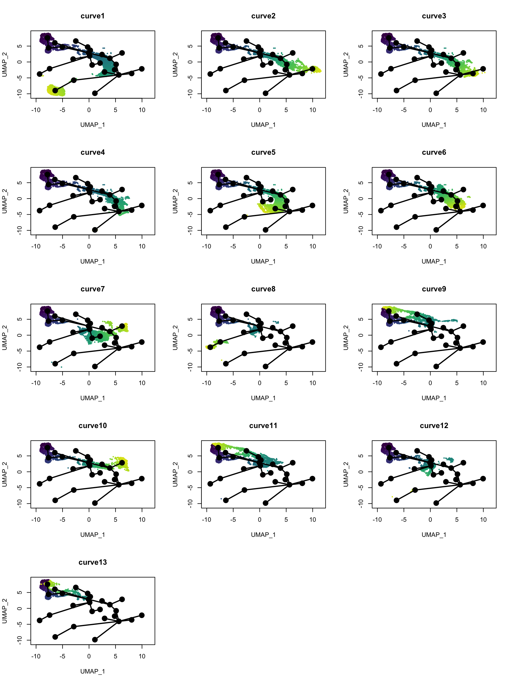
Some of the “lineages” seem spurious, especially those ending in clusters separated from the main lineage. Those may be distinct cell types of a different lineage from most cells mistaken by slingshot as highly differentiated cells from the same lineage, and SingleR does not have a reference that is detailed enough. Here manual cell type annotation with marker genes would be beneficial. Monocle 3 would have assigned disconnected trajectories to the separate clusters, but those clusters have been labeled NPCs or neurons, which must have come from neural stem cells. However, some lineages do seem reasonable, such as curves 2, 3, 5, and 7, going from qNSCs to neurons, though some lineages seem duplicated. Curves 9, 11, and 13 are saying that cell state goes back to the cluster with the qNSCs after a detour, though without more detailed manual cell type annotation, I don’t know what this means or if those “lineages” are real.
Differential expression
Let’s look at which genes are differentially expressed along one of those lineages (linage 2). In dynverse, feature (gene) importance is calculated by using gene expression to predict pseudotime value with random forest and finding genes that contribute the most to the accuracy of the response. Since it’s really not straightforward to convert existing pseudotime results to dynverse format, it would be easier to build a random forest model. Variable importance will be calculated for the top 300 highly variable genes here, with tidymodels.
# Get top highly variable genes
top_hvg <- HVFInfo(seu) %>%
  mutate(., bc = rownames(.)) %>%
  arrange(desc(residual_variance)) %>%
  top_n(300, residual_variance) %>%
  pull(bc)
# Prepare data for random forest
dat_use <- t(GetAssayData(seu, slot = "data")[top_hvg,])
dat_use_df <- cbind(slingPseudotime(sds)[,2], dat_use) # Do curve 2, so 2nd columnn
colnames(dat_use_df)[1] <- "pseudotime"
dat_use_df <- as.data.frame(dat_use_df[!is.na(dat_use_df[,1]),])
The subset of data is randomly split into training and validation; the model fitted on the training set will be evaluated on the validation set.
dat_split <- initial_split(dat_use_df)
dat_train <- training(dat_split)
dat_val <- testing(dat_split)
tidymodels is a unified interface to different machine learning models, a “tidier” version of caret. The code chunk below can easily be adjusted to use other random forest packages as the back end, so no need to learn new syntax for those packages.
model <- rand_forest(mtry = 200, trees = 1400, min_n = 15, mode = "regression") %>%
  set_engine("ranger", importance = "impurity", num.threads = 3) %>%
  fit(pseudotime ~ ., data = dat_train)
The model is evaluated on the validation set with 3 metrics: room mean squared error (RMSE), coefficient of determination using correlation (rsq, between 0 and 1), and mean absolute error (MAE).
val_results <- dat_val %>%
  mutate(estimate = predict(model, .[,-1]) %>% pull()) %>%
  select(truth = pseudotime, estimate)
metrics(data = val_results, truth, estimate)
#> # A tibble: 3 x 3
#> .metric .estimator .estimate
#> <chr> <chr> <dbl>
#> 1 rmse standard 1.37
#> 2 rsq standard 0.969
#> 3 mae standard 0.667RMSE and MAE should have the same unit as the data. As pseudotime values here usually have values much larger than 2, the error isn’t too bad. Correlation (rsq) between slingshot’s pseudotime and random forest’s prediction is very high, also showing good prediction from the top 300 highly variable genes.
summary(dat_use_df$pseudotime)#> Min. 1st Qu. Median Mean 3rd Qu. Max.
#> 0.000 4.172 13.385 11.914 18.177 24.116Now it’s time to plot some genes deemed the most important to predicting pseudotime:
var_imp <- sort(model$fit$variable.importance, decreasing = TRUE)
top_genes <- names(var_imp)[1:6]
# Convert to gene symbol
top_gene_name <- gns$gene_name[match(top_genes, gns$gene)]
par(mfrow = c(3, 2))
for (i in seq_along(top_genes)) {
colors <- pal[cut(dat_use[,top_genes[i]], breaks = 100)]
plot(reducedDim(sds), col = colors,
pch = 16, cex = 0.5, main = top_gene_name[i])
lines(sds, lwd = 2, col = 'black', type = 'lineages')
}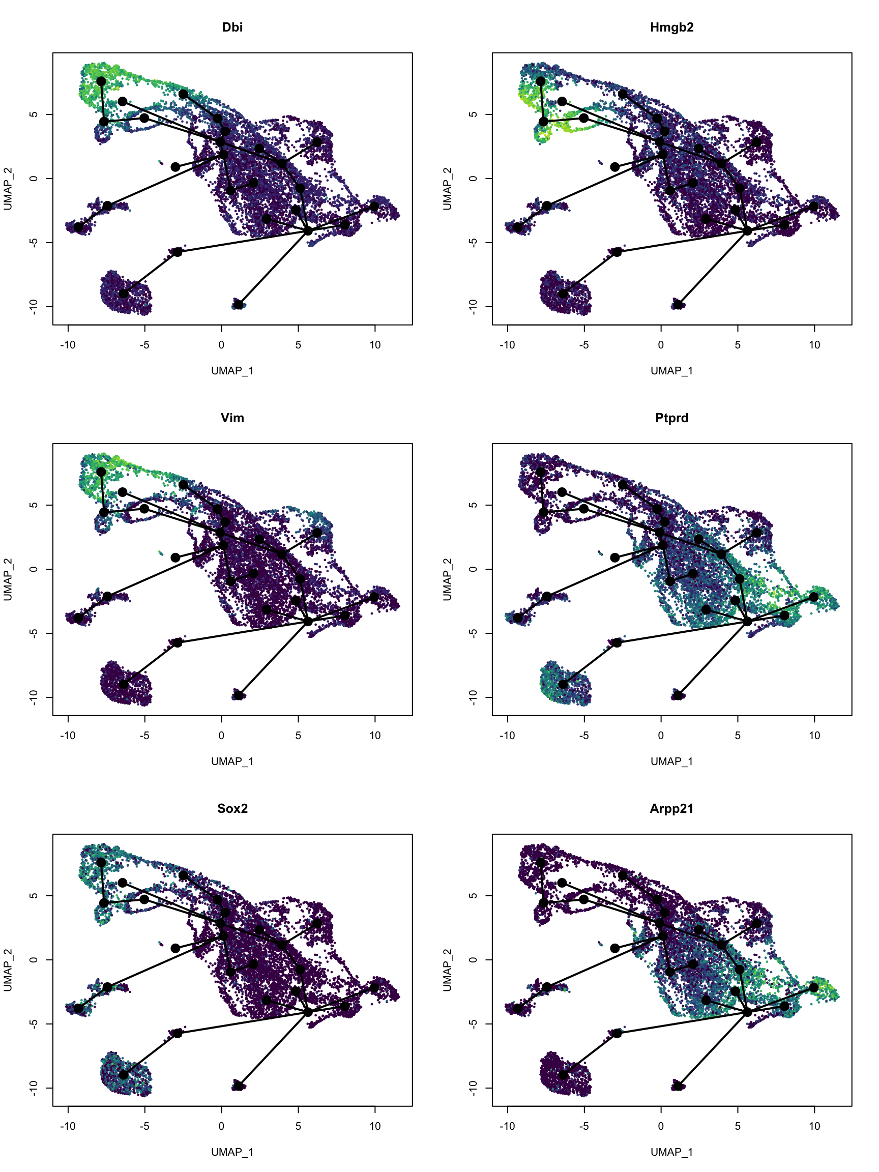
These genes do highlight different parts of the trajectory. A quick search on PubMed did show relevance of these genes to development of the central nervous system in mice.
sessionInfo()#> R version 3.6.1 (2019-07-05)
#> Platform: x86_64-apple-darwin15.6.0 (64-bit)
#> Running under: macOS Mojave 10.14.6
#>
#> Matrix products: default
#> BLAS: /Library/Frameworks/R.framework/Versions/3.6/Resources/lib/libRblas.0.dylib
#> LAPACK: /Library/Frameworks/R.framework/Versions/3.6/Resources/lib/libRlapack.dylib
#>
#> locale:
#> [1] en_US.UTF-8/en_US.UTF-8/en_US.UTF-8/C/en_US.UTF-8/en_US.UTF-8
#>
#> attached base packages:
#> [1] stats graphics grDevices utils datasets methods base
#>
#> other attached packages:
#> [1] Matrix_1.2-17 viridis_0.5.1 viridisLite_0.3.0
#> [4] Seurat_3.0.3.9024 yardstick_0.0.3 rsample_0.0.5
#> [7] recipes_0.1.6 parsnip_0.0.3.1 infer_0.4.0.1
#> [10] dials_0.0.2 scales_1.0.0 broom_0.5.2
#> [13] tidymodels_0.0.2 forcats_0.4.0 stringr_1.4.0
#> [16] dplyr_0.8.3 purrr_0.3.2 readr_1.3.1
#> [19] tidyr_0.8.3 tibble_2.1.3 ggplot2_3.2.1
#> [22] tidyverse_1.2.1 BUSpaRse_0.99.18 slingshot_1.3.1
#> [25] princurve_2.1.4
#>
#> loaded via a namespace (and not attached):
#> [1] rappdirs_0.3.1 SnowballC_0.6.0
#> [3] rtracklayer_1.45.2 R.methodsS3_1.7.1
#> [5] bit64_0.9-7 knitr_1.24
#> [7] irlba_2.3.3 dygraphs_1.1.1.6
#> [9] DelayedArray_0.11.4 R.utils_2.9.0
#> [11] data.table_1.12.2 rpart_4.1-15
#> [13] inline_0.3.15 RCurl_1.95-4.12
#> [15] AnnotationFilter_1.9.0 generics_0.0.2
#> [17] metap_1.1 BiocGenerics_0.31.5
#> [19] GenomicFeatures_1.37.4 callr_3.3.1
#> [21] cowplot_1.0.0 RSQLite_2.1.2
#> [23] RANN_2.6.1 future_1.14.0
#> [25] bit_1.1-14 tokenizers_0.2.1
#> [27] webshot_0.5.1 xml2_1.2.2
#> [29] lubridate_1.7.4 httpuv_1.5.1
#> [31] StanHeaders_2.18.1-10 SummarizedExperiment_1.15.5
#> [33] assertthat_0.2.1 gower_0.2.1
#> [35] xfun_0.8 hms_0.5.0
#> [37] bayesplot_1.7.0 evaluate_0.14
#> [39] promises_1.0.1 fansi_0.4.0
#> [41] progress_1.2.2 caTools_1.17.1.2
#> [43] dbplyr_1.4.2 readxl_1.3.1
#> [45] igraph_1.2.4.1 DBI_1.0.0
#> [47] htmlwidgets_1.3 stats4_3.6.1
#> [49] RSpectra_0.15-0 crosstalk_1.0.0
#> [51] backports_1.1.4 markdown_1.1
#> [53] gbRd_0.4-11 RcppParallel_4.4.3
#> [55] biomaRt_2.41.7 vctrs_0.2.0
#> [57] SingleCellExperiment_1.7.0 Biobase_2.45.0
#> [59] ensembldb_2.9.2 ROCR_1.0-7
#> [61] withr_2.1.2 BSgenome_1.53.0
#> [63] sctransform_0.2.0 GenomicAlignments_1.21.4
#> [65] xts_0.11-2 prettyunits_1.0.2
#> [67] cluster_2.1.0 ape_5.3
#> [69] lazyeval_0.2.2 crayon_1.3.4
#> [71] labeling_0.3 pkgconfig_2.0.2
#> [73] GenomeInfoDb_1.21.1 nlme_3.1-141
#> [75] ProtGenerics_1.17.2 nnet_7.3-12
#> [77] rlang_0.4.0 globals_0.12.4
#> [79] miniUI_0.1.1.1 colourpicker_1.0
#> [81] BiocFileCache_1.9.1 rsvd_1.0.2
#> [83] modelr_0.1.5 tidytext_0.2.2
#> [85] cellranger_1.1.0 rprojroot_1.3-2
#> [87] lmtest_0.9-37 matrixStats_0.54.0
#> [89] loo_2.1.0 boot_1.3-23
#> [91] zoo_1.8-6 base64enc_0.1-3
#> [93] whisker_0.3-2 ggridges_0.5.1
#> [95] processx_3.4.1 png_0.1-7
#> [97] bitops_1.0-6 R.oo_1.22.0
#> [99] KernSmooth_2.23-15 pROC_1.15.3
#> [101] Biostrings_2.53.2 blob_1.2.0
#> [103] rgl_0.100.26 workflowr_1.4.0
#> [105] manipulateWidget_0.10.0 shinystan_2.5.0
#> [107] S4Vectors_0.23.17 ica_1.0-2
#> [109] memoise_1.1.0 magrittr_1.5
#> [111] plyr_1.8.4 gplots_3.0.1.1
#> [113] bibtex_0.4.2 gdata_2.18.0
#> [115] zlibbioc_1.31.0 threejs_0.3.1
#> [117] compiler_3.6.1 lsei_1.2-0
#> [119] rstantools_1.5.1 RColorBrewer_1.1-2
#> [121] lme4_1.1-21 fitdistrplus_1.0-14
#> [123] Rsamtools_2.1.3 cli_1.1.0
#> [125] XVector_0.25.0 listenv_0.7.0
#> [127] pbapply_1.4-1 janeaustenr_0.1.5
#> [129] ps_1.3.0 MASS_7.3-51.4
#> [131] tidyselect_0.2.5 stringi_1.4.3
#> [133] yaml_2.2.0 askpass_1.1
#> [135] ggrepel_0.8.1 grid_3.6.1
#> [137] tidypredict_0.4.2 tools_3.6.1
#> [139] future.apply_1.3.0 parallel_3.6.1
#> [141] rstudioapi_0.10 git2r_0.26.1
#> [143] gridExtra_2.3 prodlim_2018.04.18
#> [145] plyranges_1.5.12 Rtsne_0.15
#> [147] digest_0.6.20 shiny_1.3.2
#> [149] lava_1.6.6 Rcpp_1.0.2
#> [151] GenomicRanges_1.37.14 SDMTools_1.1-221.1
#> [153] later_0.8.0 RcppAnnoy_0.0.12
#> [155] httr_1.4.1 AnnotationDbi_1.47.0
#> [157] rsconnect_0.8.15 npsurv_0.4-0
#> [159] Rdpack_0.11-0 colorspace_1.4-1
#> [161] ranger_0.11.2 reticulate_1.13
#> [163] rvest_0.3.4 XML_3.98-1.20
#> [165] fs_1.3.1 IRanges_2.19.10
#> [167] splines_3.6.1 uwot_0.1.3
#> [169] shinythemes_1.1.2 plotly_4.9.0
#> [171] xtable_1.8-4 rstanarm_2.18.2
#> [173] jsonlite_1.6 nloptr_1.2.1
#> [175] timeDate_3043.102 rstan_2.19.2
#> [177] zeallot_0.1.0 ipred_0.9-9
#> [179] R6_2.4.0 pillar_1.4.2
#> [181] htmltools_0.3.6 mime_0.7
#> [183] glue_1.3.1 minqa_1.2.4
#> [185] DT_0.8 BiocParallel_1.19.0
#> [187] class_7.3-15 codetools_0.2-16
#> [189] utf8_1.1.4 tsne_0.1-3
#> [191] pkgbuild_1.0.4 furrr_0.1.0
#> [193] lattice_0.20-38 curl_4.0
#> [195] leiden_0.3.1 gtools_3.8.1
#> [197] tidyposterior_0.0.2 shinyjs_1.0
#> [199] openssl_1.4.1 survival_2.44-1.1
#> [201] rmarkdown_1.14 munsell_0.5.0
#> [203] GenomeInfoDbData_1.2.1 haven_2.1.1
#> [205] reshape2_1.4.3 gtable_0.3.0