Processing kallisto bus Output (10x v2 chemistry)
Lambda Moses
2018-12-14
Last updated: 2018-12-14
workflowr checks: (Click a bullet for more information)-
✔ R Markdown file: up-to-date
Great! Since the R Markdown file has been committed to the Git repository, you know the exact version of the code that produced these results.
-
✔ Environment: empty
Great job! The global environment was empty. Objects defined in the global environment can affect the analysis in your R Markdown file in unknown ways. For reproduciblity it’s best to always run the code in an empty environment.
-
✔ Seed:
set.seed(20181214)The command
set.seed(20181214)was run prior to running the code in the R Markdown file. Setting a seed ensures that any results that rely on randomness, e.g. subsampling or permutations, are reproducible. -
✔ Session information: recorded
Great job! Recording the operating system, R version, and package versions is critical for reproducibility.
-
Great! You are using Git for version control. Tracking code development and connecting the code version to the results is critical for reproducibility. The version displayed above was the version of the Git repository at the time these results were generated.✔ Repository version: 1fc3e91
Note that you need to be careful to ensure that all relevant files for the analysis have been committed to Git prior to generating the results (you can usewflow_publishorwflow_git_commit). workflowr only checks the R Markdown file, but you know if there are other scripts or data files that it depends on. Below is the status of the Git repository when the results were generated:
Note that any generated files, e.g. HTML, png, CSS, etc., are not included in this status report because it is ok for generated content to have uncommitted changes.Ignored files: Ignored: .Rhistory Ignored: .Rproj.user/ Ignored: data/fastqs/ Ignored: data/hgmm_1k_fastqs.tar Ignored: data/hs_cdna.fa.gz Ignored: data/mm_cdna.fa.gz Ignored: data/whitelist_v2.txt Ignored: output/hs_mm_tr_index.idx Ignored: output/out_hgmm1k/
Expand here to see past versions:
In this vignette, we process fastq data from scRNA-seq (10x v2 chemistry) to make a sparse matrix that can be used in downstream analysis. In this vignette, we will start that standard downstream analysis with Seurat.
Download data
The data set we are using here is 1k 1:1 Mixture of Fresh Frozen Human (HEK293T) and Mouse (NIH3T3) Cells from the 10x website. First, we download the fastq files (6.34 GB).
download.file("http://cf.10xgenomics.com/samples/cell-exp/2.1.0/hgmm_1k/hgmm_1k_fastqs.tar", destfile = "./data/hgmm_1k_fastqs.tar", quiet = TRUE)Then untar this file
cd ./data
tar -xvf ./hgmm_1k_fastqs.tar
Build the kallisto index
Here we use kallisto (see this link for install instructions) to pseudoalign the reads to the transcriptome and then to create the bus file to be converted to a sparse matrix. The first step is to build an index of the transcriptome. This data set has both human and mouse cells, so we need both human and mouse transcriptomes.
# Human transcriptome
download.file("ftp://ftp.ensembl.org/pub/release-94/fasta/homo_sapiens/cdna/Homo_sapiens.GRCh38.cdna.all.fa.gz", "./data/hs_cdna.fa.gz", quiet = TRUE)
# Mouse transcriptome
download.file("ftp://ftp.ensembl.org/pub/release-94/fasta/mus_musculus/cdna/Mus_musculus.GRCm38.cdna.all.fa.gz", "./data/mm_cdna.fa.gz", quiet = TRUE)
kallisto version
#> kallisto, version 0.45.0Actually, we don’t need to unzip the fasta files
kallisto index -i ./output/hs_mm_tr_index.idx ./data/hs_cdna.fa.gz ./data/mm_cdna.fa.gzRun kallisto bus
Here we will generate the bus file. These are the technologies supported by kallisto bus:
system("kallisto bus --list")Here we have 8 samples. Each sample has 3 files: I1 means sample index, R1 means barcode and UMI, and R2 means the piece of cDNA. The -i argument specifies the index file we just built. The -o argument specifies the output directory. The -x argument specifies the sequencing technology used to generate this data set. The -t argument specifies the number of threads used.
cd ./data
kallisto bus -i ../output/hs_mm_tr_index.idx -o ../output/out_hgmm1k -x 10xv2 -t8 \
./fastqs/hgmm_1k_S1_L001_R1_001.fastq.gz ./fastqs/hgmm_1k_S1_L001_R2_001.fastq.gz \
./fastqs/hgmm_1k_S1_L002_R1_001.fastq.gz ./fastqs/hgmm_1k_S1_L002_R2_001.fastq.gz \
./fastqs/hgmm_1k_S1_L003_R1_001.fastq.gz ./fastqs/hgmm_1k_S1_L003_R2_001.fastq.gz \
./fastqs/hgmm_1k_S1_L004_R1_001.fastq.gz ./fastqs/hgmm_1k_S1_L004_R2_001.fastq.gz \
./fastqs/hgmm_1k_S1_L005_R1_001.fastq.gz ./fastqs/hgmm_1k_S1_L005_R2_001.fastq.gz \
./fastqs/hgmm_1k_S1_L006_R1_001.fastq.gz ./fastqs/hgmm_1k_S1_L006_R2_001.fastq.gz \
./fastqs/hgmm_1k_S1_L007_R1_001.fastq.gz ./fastqs/hgmm_1k_S1_L007_R2_001.fastq.gz \
./fastqs/hgmm_1k_S1_L008_R1_001.fastq.gz ./fastqs/hgmm_1k_S1_L008_R2_001.fastq.gz
See what are the outputs
list.files("./output/out_hgmm1k/")
#> [1] "matrix.ec"         "output.bus"        "output.sorted"
#> [4] "output.sorted.txt" "run_info.json"     "transcripts.txt"
Running BUStools
The output.bus file is a binary. In order to make R parse it, we need to convert it into a sorted text file. There’s a command line tool bustools for this.
# Add where I installed bustools to PATH
export PATH=$PATH:/home/lambda/mylibs/bin/
# Sort
bustools sort -o ./output/out_hgmm1k/output.sorted -t8 ./output/out_hgmm1k/output.bus
# Convert sorted file to text
bustools text -o ./output/out_hgmm1k/output.sorted.txt ./output/out_hgmm1k/output.sorted
Mapping transcripts to genes
library(BUStoolsR)For the sparse matrix, we are interested in how many UMIs per gene per cell, rather than per transcript. Remember in the output of kallisto bus, there’s the file transcripts.txt. Those are the transcripts in the transcriptome index. Now we’ll only keep the transcripts present there and make sure that the transcripts in tr2g are in the same order as those in the index. This function might be a bit slow; what’s slow is the biomart query, not processing data frames.
Note that the function transcript2gene only works for organisms that have gene and transcript IDs in Ensembl, since behind the scene, it’s using biomart to query Ensembl.
tr2g <- transcript2gene(c("Homo sapiens", "Mus musculus"),
                        kallisto_out_path = "./output/out_hgmm1k")
Mapping ECs to genes
The 3rd column in the output.sorted.txt is the equivalence class index of each UMI for each cell barcode. Equivalence class (EC) means the set of transcripts in the transcriptome that the read is compatible to. While in most cases, an EC only has transcripts for the same gene, there are some ECs that have transcripts for different genes. The file in the kallisto bus output, matrix.ec, maps the EC index in output.sorted.txt to sets of line numbers in the transcriptome assembly. That’s why we ensured that the tr2g data frame has the same order as the transcripts in the index.
genes <- EC2gene(tr2g, "./output/out_hgmm1k", ncores = 10, verbose = FALSE)Now for each EC, we have a set of genes the EC is compatible to.
Making the sparse matrix
library(data.table)For 10x, we do have a file with all valid cell barcodes that comes with CellRanger.
# Copy v2 chemistry whitelist to working directory
cp /home/lambda/cellranger-3.0.1/cellranger-cs/3.0.1/lib/python/cellranger/barcodes/737K-august-2016.txt \
./data/whitelist_v2.txt
# Read in the whitelist
whitelist_v2 <- fread("./data/whitelist_v2.txt", header = FALSE)$V1Now we have everything we need to make the sparse matrix. This function reads in output.sorted.txt line by line and processes them. It does not do barcode correction for now, so the barcode must exactly match those in the whitelist if one is provided. It took 5 to 6 minutes to construct the sparse matrix in the hgmm6k dataset, which has over 280 million lines in output.sorted.txt, which is over 9GB. Here the data set is smaller, so it’s not taking as long.
res_mat <- make_sparse_matrix("./output/out_hgmm1k/output.sorted.txt",
                              genes = genes, est_ncells = 1500,
                              est_ngenes = nrow(tr2g),
                              whitelist = whitelist_v2)
#> Reading data
#> Read 5 million lines
#> Read 10 million lines
#> Read 15 million lines
#> Read 20 million lines
#> Read 25 million lines
#> Read 30 million lines
#> Read 35 million lines
#> Read 40 million lines
#> Constructing sparse matrix
Explore the data
library(Seurat)
library(tidyverse)
#> ── Attaching packages ────────────────────────────────────────────── tidyverse 1.2.1 ──
#> ✔ ggplot2 3.1.0     ✔ purrr   0.2.5
#> ✔ tibble  1.4.2     ✔ dplyr   0.7.8
#> ✔ tidyr   0.8.2     ✔ stringr 1.3.1
#> ✔ readr   1.3.0     ✔ forcats 0.3.0
#> ── Conflicts ───────────────────────────────────────────────── tidyverse_conflicts() ──
#> ✖ dplyr::between()   masks data.table::between()
#> ✖ dplyr::filter()    masks stats::filter()
#> ✖ dplyr::first()     masks data.table::first()
#> ✖ dplyr::lag()       masks stats::lag()
#> ✖ dplyr::last()      masks data.table::last()
#> ✖ purrr::transpose() masks data.table::transpose()
library(parallel)
library(Matrix)
#>
#> Attaching package: 'Matrix'
#> The following object is masked from 'package:tidyr':
#>
#>     expand
Filter data
Cool, so now we have the sparse matrix. What does it look like?
dim(res_mat)
#> [1]  51306 353957
That’s way more cells than we expect, which is about 1000. So what’s going on?
How many UMIs per barcode?
tot_counts <- colSums(res_mat)
summary(tot_counts)
#>    Min. 1st Qu.  Median    Mean 3rd Qu.    Max.
#>     1.0     1.0     2.0   101.8    11.0 92910.0
The vast majority of “cells” have only a few UMI detected. Those are likely to be spurious. In Seurat’s vignettes, a low cutoff is usually set to the total number of UMIs in a cell, and that depends on the sequencing depth.
bcs_use <- tot_counts > 500
tot_counts_filtered <- tot_counts[bcs_use]
hist(tot_counts_filtered, breaks = 100, main = "Histogram of nUMI")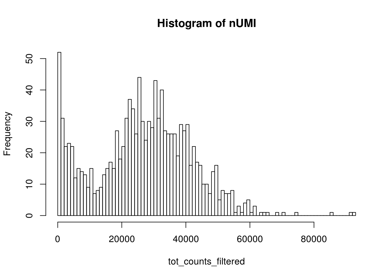
# Filter the matrix
res_mat <- res_mat[,bcs_use]
dim(res_mat)
#> [1] 51306  1176
Now this is a more reasonable number of cells.
Cell species
How many cells are from humans and how many from mice? The number of cells with mixed species indicates doublet rate.
gene_species <- ifelse(str_detect(rownames(res_mat), "^ENSMUSG"), "mouse", "human")
mouse_inds <- gene_species == "mouse"
human_inds <- gene_species == "human"
# mark cells as mouse or human
cell_species <- tibble(n_mouse_umi = colSums(res_mat[mouse_inds,]),
                       n_human_umi = colSums(res_mat[human_inds,]),
                       tot_umi = colSums(res_mat),
                       prop_mouse = n_mouse_umi / tot_umi,
                       prop_human = n_human_umi / tot_umi)
# Classify species based on proportion of UMI
cell_species <- cell_species %>%
mutate(species = case_when(
prop_mouse > 0.9 ~ "mouse",
prop_human > 0.9 ~ "human",
TRUE ~ "mixed"
))ggplot(cell_species, aes(n_human_umi, n_mouse_umi, color = species)) +
geom_point(size = 0.5) +
theme_bw()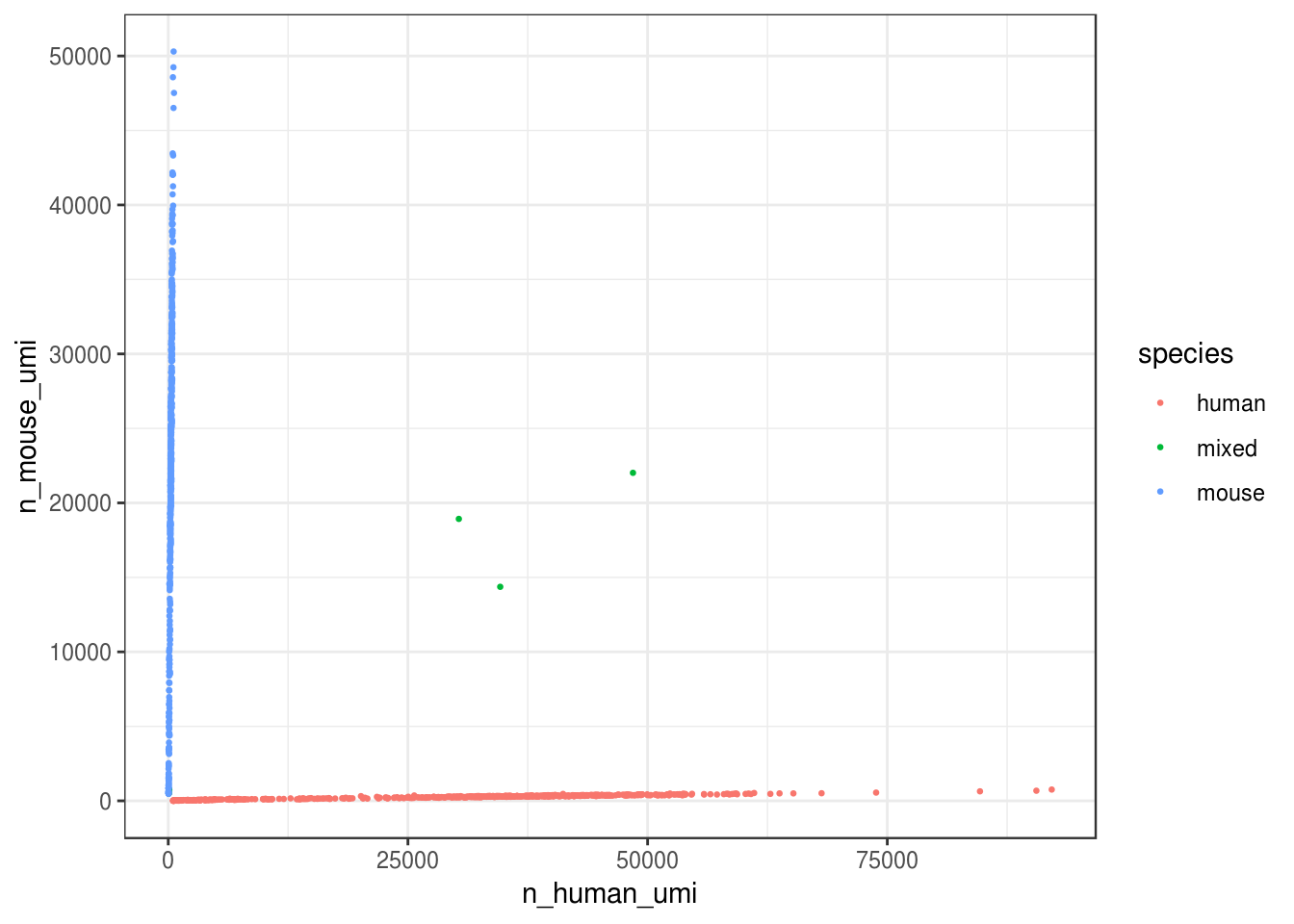
Great, looks like the vast majority of cells are not mixed.
cell_species %>%
  count(species) %>%
  mutate(proportion = n / ncol(res_mat))
#> # A tibble: 3 x 3
#>   species     n proportion
#>   <chr>   <int>      <dbl>
#> 1 human     603    0.513
#> 2 mixed       5    0.00425
#> 3 mouse     568    0.483
Great, only about 0.4% of cells here are doublets, which is lower than the ~1% 10x lists. However, doublets can still be formed with cells from the same species.
Seurat exploration
seu <- CreateSeuratObject(res_mat, min.cells = 3) %>%
  NormalizeData(verbose = FALSE) %>%
  ScaleData(verbose = FALSE) %>%
  FindVariableFeatures(verbose = FALSE)
# Add species to meta data
seu <- AddMetaData(seu, metadata = cell_species$species, col.name = "species")VlnPlot(seu, c("nCount_RNA", "nFeature_RNA"), group.by = "species")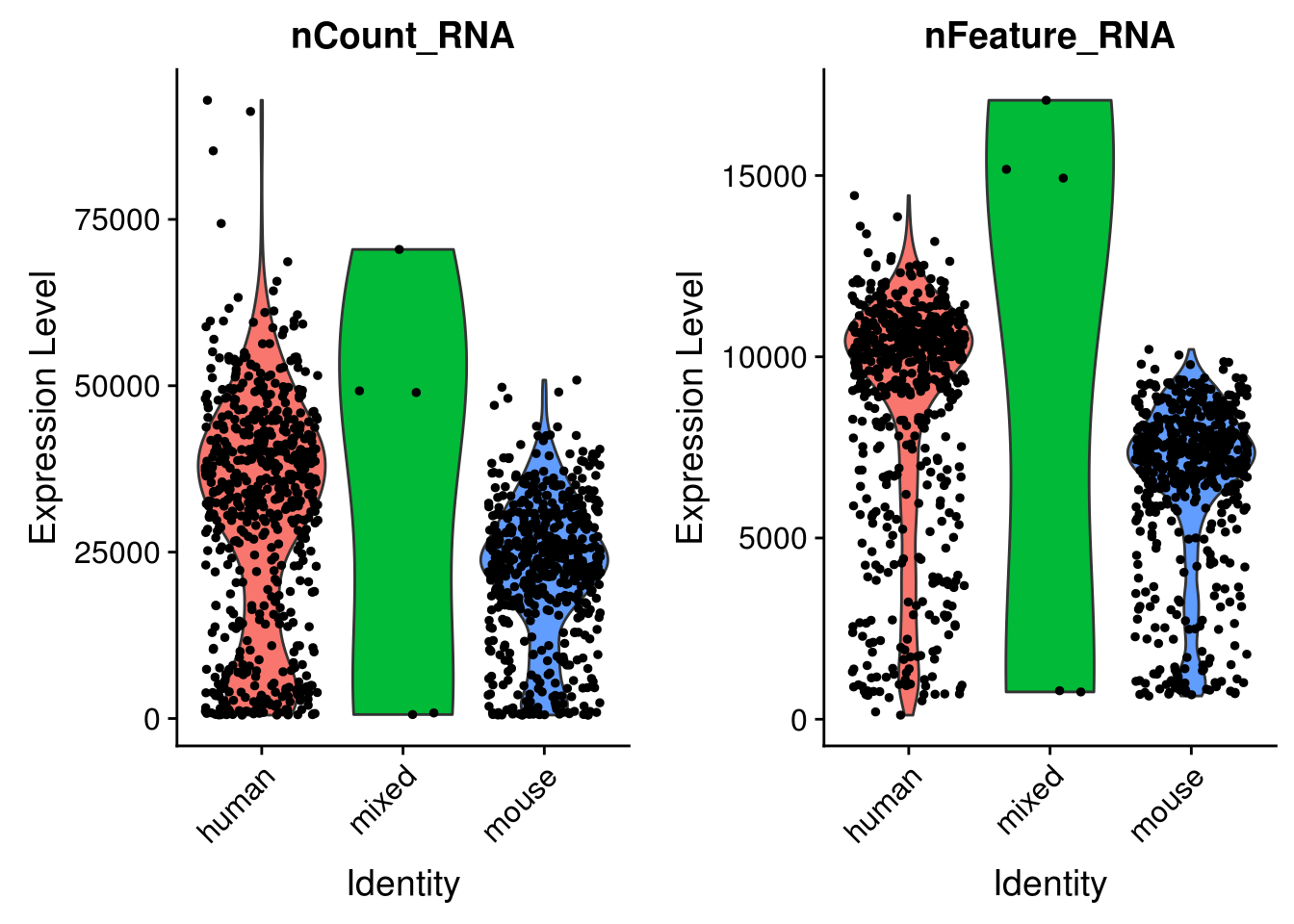
seu <- RunPCA(seu, verbose = FALSE, npcs = 30)
ElbowPlot(seu, ndims = 30)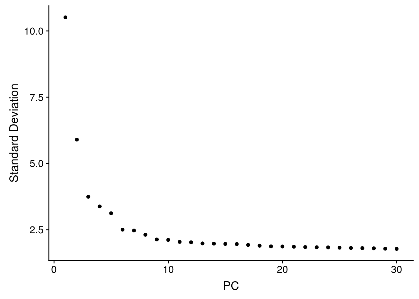
DimPlot(seu, reduction = "pca", pt.size = 0.5, group.by = "species")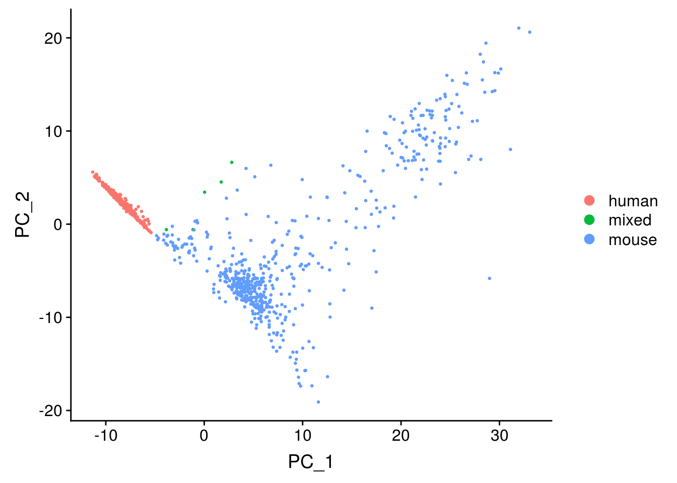
The first PC separates species, as expected.
seu <- RunTSNE(seu, dims = 1:20, check_duplicates = FALSE)
DimPlot(seu, reduction = "tsne", pt.size = 0.5, group.by = "species")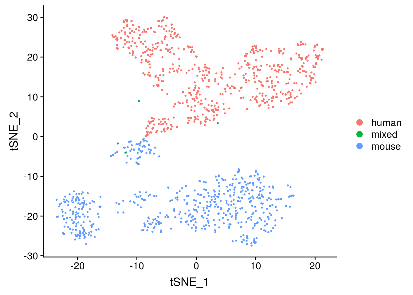
The species separate, as expected.
sessionInfo()
#> R version 3.5.1 (2018-07-02)
#> Platform: x86_64-redhat-linux-gnu (64-bit)
#> Running under: CentOS Linux 7 (Core)
#>
#> Matrix products: default
#> BLAS/LAPACK: /usr/lib64/R/lib/libRblas.so
#>
#> locale:
#>  [1] LC_CTYPE=en_US.UTF-8       LC_NUMERIC=C
#>  [3] LC_TIME=en_US.UTF-8        LC_COLLATE=en_US.UTF-8
#>  [5] LC_MONETARY=en_US.UTF-8    LC_MESSAGES=en_US.UTF-8
#>  [7] LC_PAPER=en_US.UTF-8       LC_NAME=C
#>  [9] LC_ADDRESS=C               LC_TELEPHONE=C
#> [11] LC_MEASUREMENT=en_US.UTF-8 LC_IDENTIFICATION=C
#>
#> attached base packages:
#> [1] parallel  stats     graphics  grDevices utils     datasets  methods
#> [8] base
#>
#> other attached packages:
#>  [1] bindrcpp_0.2.2    Matrix_1.2-15     forcats_0.3.0
#>  [4] stringr_1.3.1     dplyr_0.7.8       purrr_0.2.5
#>  [7] readr_1.3.0       tidyr_0.8.2       tibble_1.4.2
#> [10] ggplot2_3.1.0     tidyverse_1.2.1   Seurat_3.0.0.9000
#> [13] data.table_1.11.8 BUStoolsR_0.99.0
#>
#> loaded via a namespace (and not attached):
#>   [1] Rtsne_0.15           colorspace_1.3-2     ggridges_0.5.1
#>   [4] rprojroot_1.3-2      rstudioapi_0.8       listenv_0.7.0
#>   [7] npsurv_0.4-0         ggrepel_0.8.0        bit64_0.9-7
#>  [10] fansi_0.4.0          AnnotationDbi_1.42.1 lubridate_1.7.4
#>  [13] xml2_1.2.0           codetools_0.2-15     splines_3.5.1
#>  [16] R.methodsS3_1.7.1    lsei_1.2-0           knitr_1.21
#>  [19] zeallot_0.1.0        jsonlite_1.6         workflowr_1.1.1
#>  [22] broom_0.5.1          ica_1.0-2            cluster_2.0.7-1
#>  [25] png_0.1-7            R.oo_1.22.0          compiler_3.5.1
#>  [28] httr_1.4.0           backports_1.1.2      assertthat_0.2.0
#>  [31] lazyeval_0.2.1       cli_1.0.1            htmltools_0.3.6
#>  [34] prettyunits_1.0.2    tools_3.5.1          rsvd_1.0.0
#>  [37] igraph_1.2.2         gtable_0.2.0         glue_1.3.0
#>  [40] RANN_2.6             Rcpp_1.0.0           Biobase_2.42.0
#>  [43] cellranger_1.1.0     gdata_2.18.0         nlme_3.1-137
#>  [46] gbRd_0.4-11          lmtest_0.9-36        xfun_0.4
#>  [49] globals_0.12.4       rvest_0.3.2          irlba_2.3.2
#>  [52] gtools_3.8.1         XML_3.98-1.16        future_1.10.0
#>  [55] MASS_7.3-51.1        zoo_1.8-4            scales_1.0.0
#>  [58] hms_0.4.2            RColorBrewer_1.1-2   yaml_2.2.0
#>  [61] curl_3.2             memoise_1.1.0        reticulate_1.10
#>  [64] pbapply_1.3-4        biomaRt_2.38.0       stringi_1.2.4
#>  [67] RSQLite_2.1.1        S4Vectors_0.20.1     caTools_1.17.1.1
#>  [70] BiocGenerics_0.28.0  bibtex_0.4.2         Rdpack_0.10-1
#>  [73] SDMTools_1.1-221     rlang_0.3.0.1        pkgconfig_2.0.2
#>  [76] bitops_1.0-6         evaluate_0.12        lattice_0.20-38
#>  [79] ROCR_1.0-7           bindr_0.1.1          labeling_0.3
#>  [82] htmlwidgets_1.3      cowplot_0.9.3        bit_1.1-14
#>  [85] tidyselect_0.2.5     plyr_1.8.4           magrittr_1.5
#>  [88] R6_2.3.0             IRanges_2.16.0       gplots_3.0.1
#>  [91] generics_0.0.2       DBI_1.0.0            withr_2.1.2
#>  [94] pillar_1.3.0         haven_2.0.0          whisker_0.3-2
#>  [97] fitdistrplus_1.0-11  survival_2.43-3      RCurl_1.95-4.11
#> [100] future.apply_1.0.1   tsne_0.1-3           modelr_0.1.2
#> [103] crayon_1.3.4         utf8_1.1.4           KernSmooth_2.23-15
#> [106] plotly_4.8.0         rmarkdown_1.11       progress_1.2.0
#> [109] readxl_1.1.0         grid_3.5.1           blob_1.1.1
#> [112] git2r_0.23.0         metap_1.0            digest_0.6.18
#> [115] R.utils_2.7.0        stats4_3.5.1         munsell_0.5.0
#> [118] viridisLite_0.3.0
Session information
sessionInfo()
#> R version 3.5.1 (2018-07-02)
#> Platform: x86_64-redhat-linux-gnu (64-bit)
#> Running under: CentOS Linux 7 (Core)
#>
#> Matrix products: default
#> BLAS/LAPACK: /usr/lib64/R/lib/libRblas.so
#>
#> locale:
#>  [1] LC_CTYPE=en_US.UTF-8       LC_NUMERIC=C
#>  [3] LC_TIME=en_US.UTF-8        LC_COLLATE=en_US.UTF-8
#>  [5] LC_MONETARY=en_US.UTF-8    LC_MESSAGES=en_US.UTF-8
#>  [7] LC_PAPER=en_US.UTF-8       LC_NAME=C
#>  [9] LC_ADDRESS=C               LC_TELEPHONE=C
#> [11] LC_MEASUREMENT=en_US.UTF-8 LC_IDENTIFICATION=C
#>
#> attached base packages:
#> [1] parallel  stats     graphics  grDevices utils     datasets  methods
#> [8] base
#>
#> other attached packages:
#>  [1] bindrcpp_0.2.2    Matrix_1.2-15     forcats_0.3.0
#>  [4] stringr_1.3.1     dplyr_0.7.8       purrr_0.2.5
#>  [7] readr_1.3.0       tidyr_0.8.2       tibble_1.4.2
#> [10] ggplot2_3.1.0     tidyverse_1.2.1   Seurat_3.0.0.9000
#> [13] data.table_1.11.8 BUStoolsR_0.99.0
#>
#> loaded via a namespace (and not attached):
#>   [1] Rtsne_0.15           colorspace_1.3-2     ggridges_0.5.1
#>   [4] rprojroot_1.3-2      rstudioapi_0.8       listenv_0.7.0
#>   [7] npsurv_0.4-0         ggrepel_0.8.0        bit64_0.9-7
#>  [10] fansi_0.4.0          AnnotationDbi_1.42.1 lubridate_1.7.4
#>  [13] xml2_1.2.0           codetools_0.2-15     splines_3.5.1
#>  [16] R.methodsS3_1.7.1    lsei_1.2-0           knitr_1.21
#>  [19] zeallot_0.1.0        jsonlite_1.6         workflowr_1.1.1
#>  [22] broom_0.5.1          ica_1.0-2            cluster_2.0.7-1
#>  [25] png_0.1-7            R.oo_1.22.0          compiler_3.5.1
#>  [28] httr_1.4.0           backports_1.1.2      assertthat_0.2.0
#>  [31] lazyeval_0.2.1       cli_1.0.1            htmltools_0.3.6
#>  [34] prettyunits_1.0.2    tools_3.5.1          rsvd_1.0.0
#>  [37] igraph_1.2.2         gtable_0.2.0         glue_1.3.0
#>  [40] RANN_2.6             Rcpp_1.0.0           Biobase_2.42.0
#>  [43] cellranger_1.1.0     gdata_2.18.0         nlme_3.1-137
#>  [46] gbRd_0.4-11          lmtest_0.9-36        xfun_0.4
#>  [49] globals_0.12.4       rvest_0.3.2          irlba_2.3.2
#>  [52] gtools_3.8.1         XML_3.98-1.16        future_1.10.0
#>  [55] MASS_7.3-51.1        zoo_1.8-4            scales_1.0.0
#>  [58] hms_0.4.2            RColorBrewer_1.1-2   yaml_2.2.0
#>  [61] curl_3.2             memoise_1.1.0        reticulate_1.10
#>  [64] pbapply_1.3-4        biomaRt_2.38.0       stringi_1.2.4
#>  [67] RSQLite_2.1.1        S4Vectors_0.20.1     caTools_1.17.1.1
#>  [70] BiocGenerics_0.28.0  bibtex_0.4.2         Rdpack_0.10-1
#>  [73] SDMTools_1.1-221     rlang_0.3.0.1        pkgconfig_2.0.2
#>  [76] bitops_1.0-6         evaluate_0.12        lattice_0.20-38
#>  [79] ROCR_1.0-7           bindr_0.1.1          labeling_0.3
#>  [82] htmlwidgets_1.3      cowplot_0.9.3        bit_1.1-14
#>  [85] tidyselect_0.2.5     plyr_1.8.4           magrittr_1.5
#>  [88] R6_2.3.0             IRanges_2.16.0       gplots_3.0.1
#>  [91] generics_0.0.2       DBI_1.0.0            withr_2.1.2
#>  [94] pillar_1.3.0         haven_2.0.0          whisker_0.3-2
#>  [97] fitdistrplus_1.0-11  survival_2.43-3      RCurl_1.95-4.11
#> [100] future.apply_1.0.1   tsne_0.1-3           modelr_0.1.2
#> [103] crayon_1.3.4         utf8_1.1.4           KernSmooth_2.23-15
#> [106] plotly_4.8.0         rmarkdown_1.11       progress_1.2.0
#> [109] readxl_1.1.0         grid_3.5.1           blob_1.1.1
#> [112] git2r_0.23.0         metap_1.0            digest_0.6.18
#> [115] R.utils_2.7.0        stats4_3.5.1         munsell_0.5.0
#> [118] viridisLite_0.3.0
This reproducible R Markdown analysis was created with workflowr 1.1.1