RNA velocity with kallisto | bus and velocyto.R
Lambda Moses
2019-07-25
Last updated: 2019-07-25
Checks: 7 0
Knit directory: BUSpaRse_notebooks/
This reproducible R Markdown analysis was created with workflowr (version 1.4.0). The Checks tab describes the reproducibility checks that were applied when the results were created. The Past versions tab lists the development history.
Great! Since the R Markdown file has been committed to the Git repository, you know the exact version of the code that produced these results.
Great job! The global environment was empty. Objects defined in the global environment can affect the analysis in your R Markdown file in unknown ways. For reproduciblity it’s best to always run the code in an empty environment.
The command set.seed(20181214) was run prior to running the code in the R Markdown file. Setting a seed ensures that any results that rely on randomness, e.g. subsampling or permutations, are reproducible.
Great job! Recording the operating system, R version, and package versions is critical for reproducibility.
Nice! There were no cached chunks for this analysis, so you can be confident that you successfully produced the results during this run.
Great job! Using relative paths to the files within your workflowr project makes it easier to run your code on other machines.
Great! You are using Git for version control. Tracking code development and connecting the code version to the results is critical for reproducibility. The version displayed above was the version of the Git repository at the time these results were generated.
Note that you need to be careful to ensure that all relevant files for the analysis have been committed to Git prior to generating the results (you can use wflow_publish or wflow_git_commit). workflowr only checks the R Markdown file, but you know if there are other scripts or data files that it depends on. Below is the status of the Git repository when the results were generated:
Ignored files:
Ignored: .Rhistory
Ignored: .Rproj.user/
Ignored: BUSpaRse_notebooks.Rproj
Ignored: data/fastqs/
Ignored: data/hgmm_100_fastqs.tar
Ignored: data/hgmm_1k_fastqs.tar
Ignored: data/hgmm_1k_v3_fastqs.tar
Ignored: data/hgmm_1k_v3_fastqs/
Ignored: data/hs_cdna.fa.gz
Ignored: data/mm_cdna.fa.gz
Ignored: data/neuron_10k_v3_fastqs.tar
Ignored: data/neuron_10k_v3_fastqs/
Ignored: data/retina/
Ignored: data/whitelist_v2.txt
Ignored: data/whitelist_v3.txt
Ignored: output/hs_mm_tr_index.idx
Ignored: output/mm_cDNA_introns_97_collapse.idx
Ignored: output/mm_tr_index.idx
Ignored: output/out_hgmm1k/
Ignored: output/out_hgmm1k_v3/
Ignored: output/out_retina/
Untracked files:
Untracked: analysis/dropseq_retina.Rmd
Untracked: output/neuron10k_collapse/
Unstaged changes:
Modified: analysis/monocle2.Rmd
Note that any generated files, e.g. HTML, png, CSS, etc., are not included in this status report because it is ok for generated content to have uncommitted changes.
These are the previous versions of the R Markdown and HTML files. If you’ve configured a remote Git repository (see ?wflow_git_remote), click on the hyperlinks in the table below to view them.
| File | Version | Author | Date | Message |
|---|---|---|---|---|
| Rmd | 54e66d4 | Lambda Moses | 2019-07-26 | Added phase portraits and fixed some embarrasingly wrong bash chunks. |
| Rmd | 342b3bf | Lambda Moses | 2019-07-26 | Reran with Ensembl 97, fixed embarrasingly wrong bash chunks, and added phase portraits |
| html | a3abb12 | Lambda Moses | 2019-07-25 | Build site. |
| Rmd | 28b6ed4 | Lambda Moses | 2019-07-25 | Changed the embarrasing title |
| html | 22204f9 | Lambda Moses | 2019-07-25 | Build site. |
| Rmd | 1bd5af5 | Lambda Moses | 2019-07-25 | RNA velocity tutorial |
In this notebook, we perform RNA velocity analysis on the 10x 10k neurons from an E18 mouse. Instead of the velocyto command line tool, we will use the kallisto | bus pipeline, which is much faster than velocyto, to quantify spliced and unspliced transcripts.
Setup
If you would like to rerun this notebook, you can git clone this repository or directly download this notebook from GitHub.
Install packages
This notebook demonstrates the use of command line tools kallisto and bustools. Please use kallisto >= 0.46, whose binary can be downloaded here. The binary of bustools can be found here.
After you download the binary, you should decompress the file (if it is tar.gz) with tar -xzvf file.tar.gz in the bash terminal, and add the directory containing the binary to PATH by export PATH=$PATH:/foo/bar, where /foo/bar is the directory of interest. Then you can directly invoke the binary on the command line as we will do in this notebook.
We will be using the R packages below. BUSpaRse is not yet on CRAN or Bioconductor. For Mac users, see the installation note for BUSpaRse. BUSpaRse will be used to generate the transcript to gene file for bustools and to read output of bustools into R. We will also use Seurat version 3 which is now on CRAN. Recently, Satija lab announced SeuratWrappers, with which we can run RNA velocity directly from Seurat. SeuratWrappers is also GitHub only at present. We need to install velocyto.R, which is GitHub only, to compute and visualize RNA velocity after quantifying spliced and unspliced transcripts.
# Install devtools if it's not already installed
if (!require(devtools)) {
install.packages("devtools")
}
# Install from GitHub
devtools::install_github("BUStools/BUSpaRse")
devtools::install_github("satijalab/seurat-wrappers")
devtools::install_github("velocyto-team/velocyto.R")This vignette uses the version of DropletUtils from Bioconductor version 3.9; the version from Bioconductor 3.8 has a different user interface. If you are using a version of R older than 3.6.0 and want to rerun this vignette, then you can adapt the knee plot code to the older version of DropletUtils, or install DropletUtils from GitHub, which I did for this notebook. BSgenome.Mmusculus.UCSC.mm10 and AnnotationHub are also on Bioconductor. Bioconductor packages can be installed as such:
if (!require(BiocManager)) {
install.packages("BiocManager")
}
BiocManager::install(c("DropletUtils", "BSgenome.Mmusculus.UCSC.mm10", "AnnotationHub"))The other packages are on CRAN.
library(BUSpaRse)
library(Seurat)
library(SeuratWrappers)
library(BSgenome.Mmusculus.UCSC.mm10)
library(AnnotationHub)
library(zeallot) # For %<-% that unpacks lists in the Python manner
library(DropletUtils)
library(tidyverse)
library(uwot) # For umap
library(GGally) # For ggpairs
library(velocyto.R)
library(SingleR)
library(scales)
library(plotly)
theme_set(theme_bw())Download data
The dataset we are using is 10x 10k neurons from an E18 mouse (almost 25 GB).
# Download data
if (!file.exists("./data/neuron_10k_v3_fastqs.tar")) {
download.file("http://s3-us-west-2.amazonaws.com/10x.files/samples/cell-exp/3.0.0/neuron_10k_v3/neuron_10k_v3_fastqs.tar", "./data/neuron_10k_v3_fastqs.tar", method = "wget", quiet = TRUE)
}Then untar the downloaded file.
cd ./data
tar -xvf ./neuron_10k_v3_fastqs.tarGenerate spliced and unspliced matrices
In order to know which reads come from spliced as opposed to unspliced transcripts, we need to see whether the reads contain intronic sequences. Thus we need to include intronic sequences in the kallisto index. This can be done with the BUSpaRse function get_velocity_files, which generates all files required to run RNA velocity with kallisto | bustools. First, we need a genome annotation to get intronic sequences. We can get genome annotation from GTF or GFF3 files from Ensembl with getGTF or getGFF from the R package biomartr, but Bioconductor provides genome annotations in its databases and package ecosystem as well. As of writing, the most recent version of Ensembl is 97. UCSC annotation can be obtained from Bioconductor package TxDb.Mmusculus.UCSC.mm10.knownGene.
# query AnnotationHub for mouse Ensembl annotation
ah <- AnnotationHub()snapshotDate(): 2019-07-10query(ah, pattern = c("Ensembl", "97", "Mus musculus", "EnsDb"))AnnotationHub with 1 record
# snapshotDate(): 2019-07-10
# names(): AH73905
# $dataprovider: Ensembl
# $species: Mus musculus
# $rdataclass: EnsDb
# $rdatadateadded: 2019-05-02
# $title: Ensembl 97 EnsDb for Mus musculus
# $description: Gene and protein annotations for Mus musculus based on ...
# $taxonomyid: 10090
# $genome: GRCm38
# $sourcetype: ensembl
# $sourceurl: http://www.ensembl.org
# $sourcesize: NA
# $tags: c("97", "AHEnsDbs", "Annotation", "EnsDb", "Ensembl",
# "Gene", "Protein", "Transcript")
# retrieve record with 'object[["AH73905"]]' # Get mouse Ensembl 97 annotation
edb <- ah[["AH73905"]]downloading 0 resourcesloading from cacherequire("ensembldb")Explaining the arguments of get_velocity_files:
X, the genome annotation, which is hereedb. Hereedbis anEnsDbobject. Other allowed inputs are: a path to a GTF file, aGRangesobject made from loading a GTF file into R, or aTxDbobject (e.g.TxDb.Mmusculus.UCSC.mm10.knownGene).L: Length of the biological read of the technology of interest. For 10x v1 and v2 chemistry,Lis 98 nt, and for v3 chemistry,Lis 91 nt. The length of flanking region around introns isL-1, to capture reads from nascent transcripts that partially map to intronic and exonic sequences.Genome: Genome, either aDNAStringSetorBSgenomeobject. Genomes of Homo sapiens and common model organisms can also be easily obtained from Bioconductor. The one used in this notebook is from the packageBSgenome.Mmusculus.UCSC.mm10. Alternatively, you can download genomes from Ensembl, RefSeq, or GenBank withbiomartr::getGenome. Make sure that the annotation and the genome use the same genome version, which is here GRCm38 (mm10).Transcriptome: While you may supply a transcriptome in the form of a path to a fasta file or aDNAStringSet, this is not required. The transcriptome can be extracted from the genome with the gene annotation. We recommend extracting the transcriptome from the genome, so the transcript IDs used in the transcriptome and the annotation (and importantly, in thetr2g.tsvfile, explained later) are guaranteed to match. In this notebook, the transcriptome is not supplied and will be extracted from the genome.isoform_action: There are two options regarding gene isoforms from alternative splicing or alternative transcription start or termination site. One is to get intronic sequences separately for each isoform, and another is to collapse all isoforms of a gene by taking the union of all exonic ranges of the gene. I’m not sure which way is better, but since in the case of alternative splicing, some intronic sequences of one isoform can actually be exonic sequences of another isoform, we will collapse isoforms here.
get_velocity_files(edb, L = 91, Genome = BSgenome.Mmusculus.UCSC.mm10,
out_path = "./output/neuron10k_collapse",
isoform_action = "collapse")For regular gene count data, we build a kallisto index for cDNAs as reads are pseudoaligned to cDNAs. Here, for RNA velocity, as reads are pseudoaligned to the flanked intronic sequences in addition to the cDNAs, the flanked intronic sequences should also be part of the kallisto index.
# Intron index
kallisto index -i ./output/mm_cDNA_introns_97_collapse.idx ./output/neuron10k_collapse/cDNA_introns.faThe initial bus file is generated the same way as in regular gene count data, except with the cDNA + flanked intron index.
cd ./data/neuron_10k_v3_fastqs
kallisto bus -i ../../output/mm_cDNA_introns_97_collapse.idx \
-o ../../output/neuron10k_collapse -x 10xv3 -t8 \
neuron_10k_v3_S1_L002_R1_001.fastq.gz neuron_10k_v3_S1_L002_R2_001.fastq.gz \
neuron_10k_v3_S1_L001_R1_001.fastq.gz neuron_10k_v3_S1_L001_R2_001.fastq.gzdo_copy <- !file.exists("./data/whitelist_v3.txt")
do_bustools <- !file.exists("./output/neuron10k_velocity/output.correct.sort.bus")
do_count <- !file.exists("./output/neuron10k_velocity/spliced/s.mtx")A barcode whitelist of all valid barcode can be used, though is not strictly required. The 10x whitelist contains all barcodes from the kit. The 10x whitelist file comes with Cell Ranger installation, and is copies to the working directory of this notebook. For bustools, the whitelist must be a text file with one column, each row of which is a valid cell barcode. The text file must not be compressed.
cp ~/cellranger-3.0.2/cellranger-cs/3.0.2/lib/python/cellranger/barcodes/3M-february-2018.txt.gz \
./data/whitelist_v3.txt.gz
# Decompress
gunzip ./data/whitelist_v3.txt.gzThe bustools correct command checks the whitelist and can correct some barcodes not on the whitelist but might have been due to sequencing error or mutation. If you do not wish to use a whitelist, then you can skip bustools correct below and go straight to bustools sort. In bash, | is a pipe just like the magrittr pipe %>% in R. The - by the end of the bustools sort command indicates where what goes through the pipe goes, i.e. the output of bustools correct is becoming the input to bustools sort. -t4 means using 4 threads.
Note: This part will change soon!
The bustools capture command determines what is from cDNA and what is from the flanked introns and generate two separate bus files.
cd ./output/neuron10k_collapse
mkdir cDNA_capture/ introns_capture/ spliced/ unspliced/
bustools correct -w ../../data/whitelist_v3.txt -p output.bus | \
bustools sort -o output.correct.sort.bus -t4 -
bustools capture -o cDNA_capture/ -c ./cDNA_tx_to_capture.txt -e matrix.ec -t transcripts.txt output.correct.sort.bus
bustools capture -o introns_capture/ -c ./introns_tx_to_capture.txt -e matrix.ec -t transcripts.txt output.correct.sort.busmkdir: cannot create directory ‘cDNA_capture/’: File exists
mkdir: cannot create directory ‘introns_capture/’: File exists
mkdir: cannot create directory ‘spliced/’: File exists
mkdir: cannot create directory ‘unspliced/’: File exists
Found 6794880 barcodes in the whitelist
Number of hamming dist 1 barcodes = 67537014
Processed 337467134 bus records
In whitelist = 325106011
Corrected = 1012838
Uncorrected = 11348285
Read in 326118849 number of busrecords
Parsing transcripts .. done
Parsing ECs .. done
Parsing capture list .. Error: could not find capture transcript ENSMUST00000051100.6 in transcript list
done
Parsing transcripts .. done
Parsing ECs .. done
Parsing capture list .. doneUnlike for just a gene count matrix, for RNA velocity, 2 matrices are generated. One for spliced reads, and the other for unspliced. Here the reads not captured for cDNA go to the unspliced matrix, and the reads not captured for introns go to the spliced matrix.
cd ./output/neuron10k_collapse
bustools count -o unspliced/u -g ./tr2g.tsv -e cDNA_capture/split.ec -t transcripts.txt --genecounts cDNA_capture/split.bus
bustools count -o spliced/s -g ./tr2g.tsv -e introns_capture/split.ec -t transcripts.txt --genecounts introns_capture/split.busPreprocessing
Remove empty droplets
Now we have the spliced and unspliced matrices to be read into R:
c(spliced, unspliced) %<-% read_velocity_output(spliced_dir = "./output/neuron10k_collapse/spliced",
spliced_name = "s",
unspliced_dir = "./output/neuron10k_collapse/unspliced",
unspliced_name = "u")The %<-% from zeallot unpacks a list of 2 into 2 separate objects in the Python and Matlab manner. How many UMIs are from unspliced transcripts?
sum(unspliced@x) / (sum(unspliced@x) + sum(spliced@x))[1] 0.530749There are more unspliced counts than spliced counts, which has been observed in multiple datasets. In contrast, for velocyto, the unspliced count is usually between 10% and 20% of the sum of spliced and unspliced. Perhaps this is because kallisto | bus counts reads that are partially intronic and partially exonic as unspliced while velocyto throws away many reads (see this GitHub issue).
We expect around 10,000 cells. There are over 10 times more barcodes here, since most barcodes are from empty droplets. The number of genes does not seem too outrageous.
dim(spliced)[1] 55487 1212424dim(unspliced)[1] 55487 1383375Most barcodes only have 0 or 1 UMIs detected.
tot_count <- Matrix::colSums(spliced)
summary(tot_count) Min. 1st Qu. Median Mean 3rd Qu. Max.
0.00 1.00 1.00 64.72 2.00 46874.00 A commonly used method to estimate the number of empty droplets is barcode ranking knee and inflection points, as those are often assumed to represent transition between two components of a distribution. While more sophisticated methods exist (e.g. see emptyDrops in DropletUtils), for simplicity, we will use the barcode ranking method here. However, whichever way we go, we don’t have the ground truth. The spliced matrix is used for filtering, though both matrices have similar inflection points.
bc_rank <- barcodeRanks(spliced)
bc_uns <- barcodeRanks(unspliced)Here the knee plot is transposed, because this is more generalizable to multi-modal data, such that those with not only RNA-seq but also abundance of cell surface markers. In that case, we can plot number of UMIs on the x axis, number of cell surface protein tags on the y axis, and barcode rank based on both UMI and protein tag counts on the z axis; it makes more sense to make barcode rank the dependent variable. See this blog post by Lior Pachter for a more detailed explanation.
tibble(rank = bc_rank$rank, total = bc_rank$total, matrix = "spliced") %>%
bind_rows(tibble(rank = bc_uns$rank, total = bc_uns$total, matrix = "unspliced")) %>%
distinct() %>%
ggplot(aes(total, rank, color = matrix)) +
geom_line() +
geom_vline(xintercept = metadata(bc_rank)$knee, color = "blue", linetype = 2) +
geom_vline(xintercept = metadata(bc_rank)$inflection, color = "green", linetype = 2) +
geom_vline(xintercept = metadata(bc_uns)$knee, color = "purple", linetype = 3) +
geom_vline(xintercept = metadata(bc_uns)$inflection, color = "cyan", linetype = 3) +
annotate("text", y = c(1000, 1000, 500, 500),
x = 1.5 * c(metadata(bc_rank)$knee, metadata(bc_rank)$inflection,
metadata(bc_uns)$knee, metadata(bc_uns)$inflectio),
label = c("knee (s)", "inflection (s)", "knee (u)", "inflection (u)"),
color = c("blue", "green", "purple", "cyan")) +
scale_x_log10() +
scale_y_log10() +
labs(y = "Rank", x = "Total UMI counts") +
theme_bw()Warning: Transformation introduced infinite values in continuous x-axis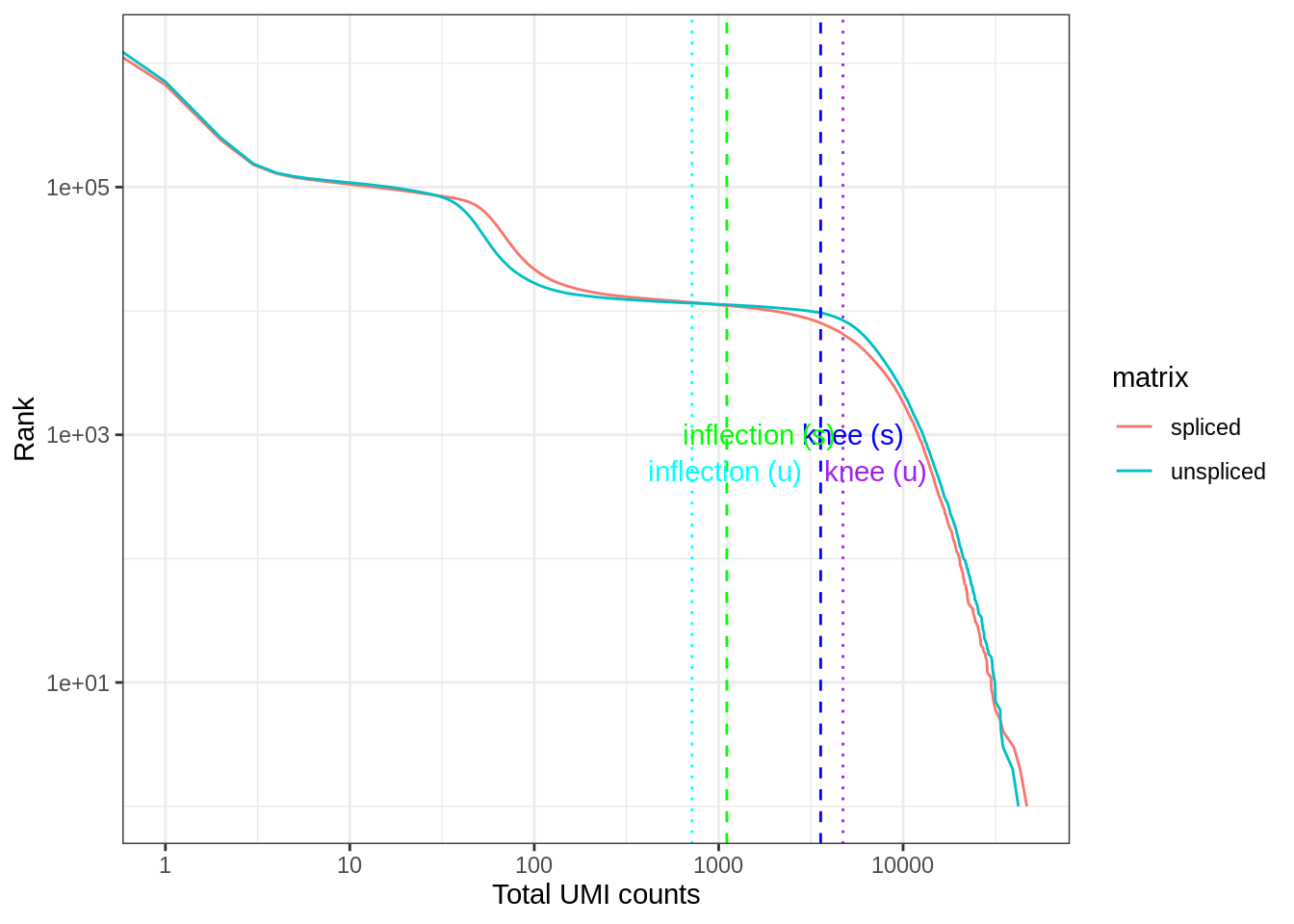
| Version | Author | Date |
|---|---|---|
| 22204f9 | Lambda Moses | 2019-07-25 |
Which inflection point should be used to remove what are supposed to be empty droplets? The one of the spliced matrix or the unspliced matrix?
Actually, spliced and unspliced counts are multimodal data, so why not make one of those promised 3D plots where the barcode rank depends on two variables? The rank (z axis) would now be the number cells with at least x spliced UMIs and y unspliced UMIs. How shall this be computed? The transposed knee plot (or rank-UMI plot) can be thought of as (1 - ECDF(total_UMI))*n_cells. In the ECDF of total UMI counts, the dependent variable is the proportion of cells with at most this number of distinct UMIs. So 1 minus that would mean the proportion of cells with at least this number of distinct UMIs. In the knee plot, the rank is the number of cells with at least this number of distinct UMIs. So dividing by the number of cells, we get 1 - ECDF(total_UMI). Would computing the 2D ECDF be more efficient than this naive approach? There is an R package that can compute bivariate ECDFs called Emcdf, but it uses so much memory that even our server can’t handle. I failed to find implementations of bivariate ECDFs in other languages. There is an algorithm based on range trees that can find multivariate ECDF efficiently.
Before obtaining a more efficient implementation, I used my naive approach that translates this concept into code very literally. Though I used Rcpp, it’s really slow. The trick to make it faster is to only evaluate how many cells have at least x spliced and y unspliced counts at a smaller number of grid points of x and y.
//[[Rcpp::depends(RcppProgress)]]
#include <progress.hpp>
#include <progress_bar.hpp>
#include <Rcpp.h>
using namespace Rcpp;
//[[Rcpp::export]]
NumericMatrix bc_ranks2(NumericVector x, NumericVector y,
NumericVector x_grid, NumericVector y_grid) {
NumericMatrix out(x_grid.size(), y_grid.size());
Progress p(x_grid.size(), true);
for (int i = 0; i < x_grid.size(); i++) {
checkUserInterrupt();
for (int j = 0; j < y_grid.size(); j++) {
out(i,j) = sum((x_grid[i] <= x) & (y_grid[j] <= y));
}
p.increment();
}
return(out);
}As most barcodes have a small number of distinct UMIs detected, the grid should be denser for fewer counts. Making the grid in log space achieves this.
# Can only plot barcodes with both spliced and unspliced counts
bcs_inter <- intersect(colnames(spliced), colnames(unspliced))
s <- colSums(spliced[,bcs_inter])
u <- colSums(unspliced[,bcs_inter])
# Grid points
sr <- sort(unique(exp(round(log(s)*100)/100)))
ur <- sort(unique(exp(round(log(u)*100)/100)))# Run naive approach
bc2 <- bc_ranks2(s, u, sr, ur)What would the “rank” look like?
# can't turn color to lot scale unless log values are plotted
z_use <- log10(bc2)
z_use[is.infinite(z_use)] <- NA
plot_ly(x = sr, y = ur, z = z_use) %>% add_surface() %>%
layout(scene = list(xaxis = list(title = "Total spliced UMIs", type = "log"),
yaxis = list(title = "Total unspliced UMIs", type = "log"),
zaxis = list(title = "Rank (log10)")))