Dorsal Horn and Ventral Lateral White DE analysis

workflowr

• Summary
• Checks
• Past versions

Last updated: 2024-10-19

Checks: 7 0

Knit directory: DEanalysis/

This reproducible R Markdown analysis was created with workflowr (version 1.7.1). The Checks tab describes the reproducibility checks that were applied when the results were created. The Past versions tab lists the development history.

---

R Markdown file: up-to-date

Great! Since the R Markdown file has been committed to the Git repository, you know the exact version of the code that produced these results.

Environment: empty

Great job! The global environment was empty. Objects defined in the global environment can affect the analysis in your R Markdown file in unknown ways. For reproduciblity it’s best to always run the code in an empty environment.

Seed: set.seed(20230508)

The command set.seed(20230508) was run prior to running the code in the R Markdown file. Setting a seed ensures that any results that rely on randomness, e.g. subsampling or permutations, are reproducible.

Session information: recorded

Great job! Recording the operating system, R version, and package versions is critical for reproducibility.

Cache: none

Nice! There were no cached chunks for this analysis, so you can be confident that you successfully produced the results during this run.

File paths: relative

Great job! Using relative paths to the files within your workflowr project makes it easier to run your code on other machines.

Repository version: b100704

Great! You are using Git for version control. Tracking code development and connecting the code version to the results is critical for reproducibility.

The results in this page were generated with repository version b100704. See the Past versions tab to see a history of the changes made to the R Markdown and HTML files.

Note that you need to be careful to ensure that all relevant files for the analysis have been committed to Git prior to generating the results (you can use wflow_publish or wflow_git_commit). workflowr only checks the R Markdown file, but you know if there are other scripts or data files that it depends on. Below is the status of the Git repository when the results were generated:

Ignored files:
    Ignored:    .Rhistory
    Ignored:    .Rproj.user/
    Ignored:    analysis/figure/
    Ignored:    data/.Rhistory

Untracked files:
    Untracked:  .DS_Store
    Untracked:  .gitignore
    Untracked:  analysis/analysis_humanspine.Rmd
    Untracked:  analysis/simulation_donor_effect.Rmd
    Untracked:  data/.DS_Store
    Untracked:  data/10X_DEresult_update.RData
    Untracked:  data/10X_DEresult_update2.RData
    Untracked:  data/10X_Kang_DEresult.RData
    Untracked:  data/10X_inputdata.RData
    Untracked:  data/10X_inputdata_DEresult.RData
    Untracked:  data/10X_inputdata_cpm.RData
    Untracked:  data/10X_inputdata_integrated.RData
    Untracked:  data/10X_inputdata_lognorm.RData
    Untracked:  data/10Xdata_annotate.rds
    Untracked:  data/Bcells.Rmd
    Untracked:  data/Bcellsce.rds
    Untracked:  data/Kang_DEresult.RData
    Untracked:  data/Kang_data.RData
    Untracked:  data/fallopian_tubes.RData
    Untracked:  data/fallopian_tubes_all.RData
    Untracked:  data/human/
    Untracked:  data/human_spine.RData
    Untracked:  data/human_spine_DEresult.RData
    Untracked:  data/mouse/
    Untracked:  data/permutation.RData
    Untracked:  data/permutation13.RData
    Untracked:  data/permutation2.RData
    Untracked:  data/splatter_simulation.RData
    Untracked:  data/splatter_simulation1.RData
    Untracked:  data/splatter_simulation2.RData
    Untracked:  data/splatter_simulation3.RData
    Untracked:  data/vstcounts.Rdata
    Untracked:  figure/

Unstaged changes:
    Modified:   analysis/.Rhistory
    Modified:   analysis/CD14+-Monocytes.Rmd
    Modified:   analysis/human_spine_overview.Rmd
    Modified:   code/DE_methods.R

Note that any generated files, e.g. HTML, png, CSS, etc., are not included in this status report because it is ok for generated content to have uncommitted changes.

---

These are the previous versions of the repository in which changes were made to the R Markdown (analysis/Dors_Horn_Vent_Lat_White.Rmd) and HTML (docs/Dors_Horn_Vent_Lat_White.html) files. If you’ve configured a remote Git repository (see ?wflow_git_remote), click on the hyperlinks in the table below to view the files as they were in that past version.

File	Version	Author	Date	Message
Rmd	b100704	C-HW	2024-10-19	workflowr::wflow_publish("./analysis/Dors_Horn_Vent_Lat_White.Rmd")

---

source("./code/hippo_all_proportion.R")
source("./code/DE_methods.R")
source("./code/functions_in_rmd.R")
# load DE result generated from "analysis_humanspine.Rmd"
load("./data/human_spine_DEresult.RData")
load("./data/human_spine.RData")
load("./data/fallopian_tubes.RData")
library(ggplot2)
library(dplyr)

Attaching package: 'dplyr'

The following objects are masked from 'package:stats':

    filter, lag

The following objects are masked from 'package:base':

    intersect, setdiff, setequal, union

library(ggpubr)
library(SingleCellExperiment)

Loading required package: SummarizedExperiment

Loading required package: MatrixGenerics

Loading required package: matrixStats

Attaching package: 'matrixStats'

The following object is masked from 'package:dplyr':

    count

Attaching package: 'MatrixGenerics'

The following objects are masked from 'package:matrixStats':

    colAlls, colAnyNAs, colAnys, colAvgsPerRowSet, colCollapse,
    colCounts, colCummaxs, colCummins, colCumprods, colCumsums,
    colDiffs, colIQRDiffs, colIQRs, colLogSumExps, colMadDiffs,
    colMads, colMaxs, colMeans2, colMedians, colMins, colOrderStats,
    colProds, colQuantiles, colRanges, colRanks, colSdDiffs, colSds,
    colSums2, colTabulates, colVarDiffs, colVars, colWeightedMads,
    colWeightedMeans, colWeightedMedians, colWeightedSds,
    colWeightedVars, rowAlls, rowAnyNAs, rowAnys, rowAvgsPerColSet,
    rowCollapse, rowCounts, rowCummaxs, rowCummins, rowCumprods,
    rowCumsums, rowDiffs, rowIQRDiffs, rowIQRs, rowLogSumExps,
    rowMadDiffs, rowMads, rowMaxs, rowMeans2, rowMedians, rowMins,
    rowOrderStats, rowProds, rowQuantiles, rowRanges, rowRanks,
    rowSdDiffs, rowSds, rowSums2, rowTabulates, rowVarDiffs, rowVars,
    rowWeightedMads, rowWeightedMeans, rowWeightedMedians,
    rowWeightedSds, rowWeightedVars

Loading required package: GenomicRanges

Loading required package: stats4

Loading required package: BiocGenerics

Attaching package: 'BiocGenerics'

The following objects are masked from 'package:dplyr':

    combine, intersect, setdiff, union

The following objects are masked from 'package:stats':

    IQR, mad, sd, var, xtabs

The following objects are masked from 'package:base':

    anyDuplicated, aperm, append, as.data.frame, basename, cbind,
    colnames, dirname, do.call, duplicated, eval, evalq, Filter, Find,
    get, grep, grepl, intersect, is.unsorted, lapply, Map, mapply,
    match, mget, order, paste, pmax, pmax.int, pmin, pmin.int,
    Position, rank, rbind, Reduce, rownames, sapply, setdiff, table,
    tapply, union, unique, unsplit, which.max, which.min

Loading required package: S4Vectors

Attaching package: 'S4Vectors'

The following objects are masked from 'package:dplyr':

    first, rename

The following object is masked from 'package:utils':

    findMatches

The following objects are masked from 'package:base':

    expand.grid, I, unname

Loading required package: IRanges

Attaching package: 'IRanges'

The following objects are masked from 'package:dplyr':

    collapse, desc, slice

Loading required package: GenomeInfoDb

Loading required package: Biobase

Welcome to Bioconductor

    Vignettes contain introductory material; view with
    'browseVignettes()'. To cite Bioconductor, see
    'citation("Biobase")', and for packages 'citation("pkgname")'.

Attaching package: 'Biobase'

The following object is masked from 'package:MatrixGenerics':

    rowMedians

The following objects are masked from 'package:matrixStats':

    anyMissing, rowMedians

library(pheatmap)
library(gridExtra)

Attaching package: 'gridExtra'

The following object is masked from 'package:Biobase':

    combine

The following object is masked from 'package:BiocGenerics':

    combine

The following object is masked from 'package:dplyr':

    combine

library(reshape)

Attaching package: 'reshape'

The following objects are masked from 'package:S4Vectors':

    expand, rename

The following object is masked from 'package:dplyr':

    rename

library(clusterProfiler)

clusterProfiler v4.12.6 Learn more at https://yulab-smu.top/contribution-knowledge-mining/

Please cite:

Guangchuang Yu, Li-Gen Wang, Yanyan Han and Qing-Yu He.
clusterProfiler: an R package for comparing biological themes among
gene clusters. OMICS: A Journal of Integrative Biology. 2012,
16(5):284-287

Attaching package: 'clusterProfiler'

The following object is masked from 'package:reshape':

    rename

The following object is masked from 'package:IRanges':

    slice

The following object is masked from 'package:S4Vectors':

    rename

The following object is masked from 'package:stats':

    filter

library(enrichplot)

Attaching package: 'enrichplot'

The following object is masked from 'package:ggpubr':

    color_palette

library("org.Hs.eg.db")

Loading required package: AnnotationDbi

Attaching package: 'AnnotationDbi'

The following object is masked from 'package:clusterProfiler':

    select

The following object is masked from 'package:dplyr':

    select

library(pathview)

##############################################################################
Pathview is an open source software package distributed under GNU General
Public License version 3 (GPLv3). Details of GPLv3 is available at
http://www.gnu.org/licenses/gpl-3.0.html. Particullary, users are required to
formally cite the original Pathview paper (not just mention it) in publications
or products. For details, do citation("pathview") within R.

The pathview downloads and uses KEGG data. Non-academic uses may require a KEGG
license agreement (details at http://www.kegg.jp/kegg/legal.html).
##############################################################################

group1 = "Dors_Horn"
group2 = "Vent_Lat_White"
pair = c(group1, group2)
subgroupsce = sce_human_spine_filtered[, sce_human_spine_filtered$region%in%pair]
subgroup_Seurat = Seurat_human_spine_integrate[, Seurat_human_spine_integrate$region%in%pair]
cellgroup = ifelse(subgroupsce$region%in% group1, 1, 2)
  genemean1 = rowMeans(counts(subgroupsce)[,cellgroup==1])
  genemean2 = rowMeans(counts(subgroupsce)[,cellgroup==2])
  subgroupsce@metadata$log2mean = log2(genemean1*genemean2)/2
  subgroupsce@metadata$log2meandiff = log2(abs(genemean1-genemean2))

Wilcox_Seurat_df$avg_log2FC = - Wilcox_Seurat_df$avg_log2FC

region_palette = c(
  "#A0522D", "#6A00FF", "#A4C400", "#F472D0",
  "#0050EF", "#00ABA9", "#F0A30A", "#008A00",
  "#647687", "#1BA1E2", "#FA6800", "#E3C800")
donors_palette <- c("#FDA4AF", "#FCD34D", "#BEF264", "#67E8F9", "#A5B4FC", 
                    "#FF6F61", "#6A4C93", "#001688", "#009A33")
names(region_palette) = levels(as.factor(sce_human_spine_filtered$region))
names(donors_palette) = levels(as.factor(sce_human_spine_filtered$patient_ID))
annotation_colors = list(Region = region_palette[c(group1, group2)], Donor = donors_palette)
remove_y = theme(
  axis.text.y = element_blank(),
  axis.ticks.y = element_blank(),
  axis.title.y = element_blank()
)

Data summary

df = data.frame(Region = subgroupsce$region, Donor = subgroupsce$patient_ID, Count = 1)
df = aggregate(df$Count, list(df$Donor, df$Region), FUN = sum)
colnames(df) = c("Donor", "Region", "Count")
df = df[nrow(df):1,]
df$cumcount= c(t(aggregate(df$Count, list(rev(df$Region)), FUN = cumsum)[,-1]))
p_donor = ggplot(df, aes(x = Region, y = Count, fill = Donor)) + 
  geom_bar(stat = "identity") + 
  xlab("Region") + 
  ylab("Number of cells") + 
  scale_fill_manual(values = donors_palette) + 
  geom_text(aes(label=Count, y = cumcount), vjust = -0.2, size = 2) + 
  theme_bw() + 
  theme(panel.grid = element_blank())

# gene count per cell by region
count_cell_df = data.frame(totalcount = apply(assays(subgroupsce)$counts, 2, sum), Region = as.factor(subgroupsce$region), Donor = as.factor(subgroupsce$patient_ID), Slide = as.factor(subgroupsce$Slide))

p_countbygroup = ggplot(count_cell_df, aes(x = totalcount, color = Region)) +
  geom_histogram(aes(y=..density..), fill= "white", alpha=0.5, position="identity") +
  geom_density(alpha = 0.2) +
  xlab("Library size") + 
  ylab("Density") +
  theme_bw() + 
  theme(panel.grid = element_blank()) +
  scale_colour_manual(values = region_palette[c(group1, group2)]) +
  xlim(c(0,5000))

# gene count per cell by donor
p_countbydonor = ggplot(count_cell_df, aes(x = totalcount, color = Donor)) +
  geom_histogram(aes(y=..density..),fill="white", alpha=0.5, position="identity") + 
  geom_density(alpha = 0.2) + 
  xlab("Library size") + 
  ylab("Density") +
  theme_bw() + 
  theme(panel.grid = element_blank()) + 
  scale_color_manual(values = donors_palette) + 
  xlim(c(0,5000))

# gene count per cell by slide
p_countbyslide = ggplot(count_cell_df, aes(x = totalcount, color = Slide)) +
  geom_histogram(aes(y=..density..),fill="white", alpha=0.5, position="identity") + 
  geom_density(alpha = 0.2) + 
  xlab("Library size") + 
  ylab("Density") +
  theme_bw() + 
  theme(panel.grid = element_blank()) + 
  xlim(c(0,5000))

# zero proportion per gene
zeroprop_df = rbind(data.frame(zero_prop = rowMeans(assays(subgroupsce)$counts[, subgroupsce$region %in% group1]== 0), genemean = rowMeans(assays(subgroupsce)$counts[, subgroupsce$region %in% group1]), Region = group1),
                data.frame(zero_prop = rowMeans(assays(subgroupsce)$counts[, subgroupsce$region %in% group2]== 0), genemean = rowMeans(assays(subgroupsce)$counts[, subgroupsce$region %in% group2]), Region = group2),
                data.frame(zero_prop = rowMeans(assays(subgroupsce)$counts == 0), genemean = rowMeans(assays(subgroupsce)$counts), Region = "Combined")
                )
zeroprop_df = zeroprop_df[which(zeroprop_df$genemean>0),]
zeroprop_df$Region =factor(zeroprop_df$Region, levels = c(group1, group2, "Combined"))

p_zeroprop = ggplot(zeroprop_df, aes(x = genemean, y = zero_prop)) + 
  geom_point(aes(shape = Region, color = Region), alpha=0.5, size = 1.2) + 
  scale_color_manual(values = c(region_palette[c(group1, group2)],Combined = "darkmagenta")) +
  scale_shape_manual(values = c(16,16,3)) +
  xlab("Gene mean") + 
  ylab("Zero proportion") +
  xlim(c(0,10)) + 
  stat_function(fun = function(x) exp(-x), colour = "black") +
  theme_bw() + theme(panel.grid = element_blank())

ggarrange(p_zeroprop, p_countbygroup, p_countbyslide, p_countbydonor, nrow = 2, ncol = 2)

Warning: Removed 17 rows containing missing values or values outside the scale range
(`geom_point()`).

Warning: The dot-dot notation (`..density..`) was deprecated in ggplot2 3.4.0.
ℹ Please use `after_stat(density)` instead.
This warning is displayed once every 8 hours.
Call `lifecycle::last_lifecycle_warnings()` to see where this warning was
generated.

`stat_bin()` using `bins = 30`. Pick better value with `binwidth`.

Warning: Removed 44 rows containing non-finite outside the scale range
(`stat_bin()`).

Warning: Removed 44 rows containing non-finite outside the scale range
(`stat_density()`).

Warning: Removed 4 rows containing missing values or values outside the scale range
(`geom_bar()`).

`stat_bin()` using `bins = 30`. Pick better value with `binwidth`.

Warning: Removed 44 rows containing non-finite outside the scale range
(`stat_bin()`).

Warning: Removed 44 rows containing non-finite outside the scale range
(`stat_density()`).

Warning: Removed 32 rows containing missing values or values outside the scale range
(`geom_bar()`).

`stat_bin()` using `bins = 30`. Pick better value with `binwidth`.

Warning: Removed 44 rows containing non-finite outside the scale range
(`stat_bin()`).

Warning: Removed 44 rows containing non-finite outside the scale range
(`stat_density()`).

Warning: Removed 18 rows containing missing values or values outside the scale range
(`geom_bar()`).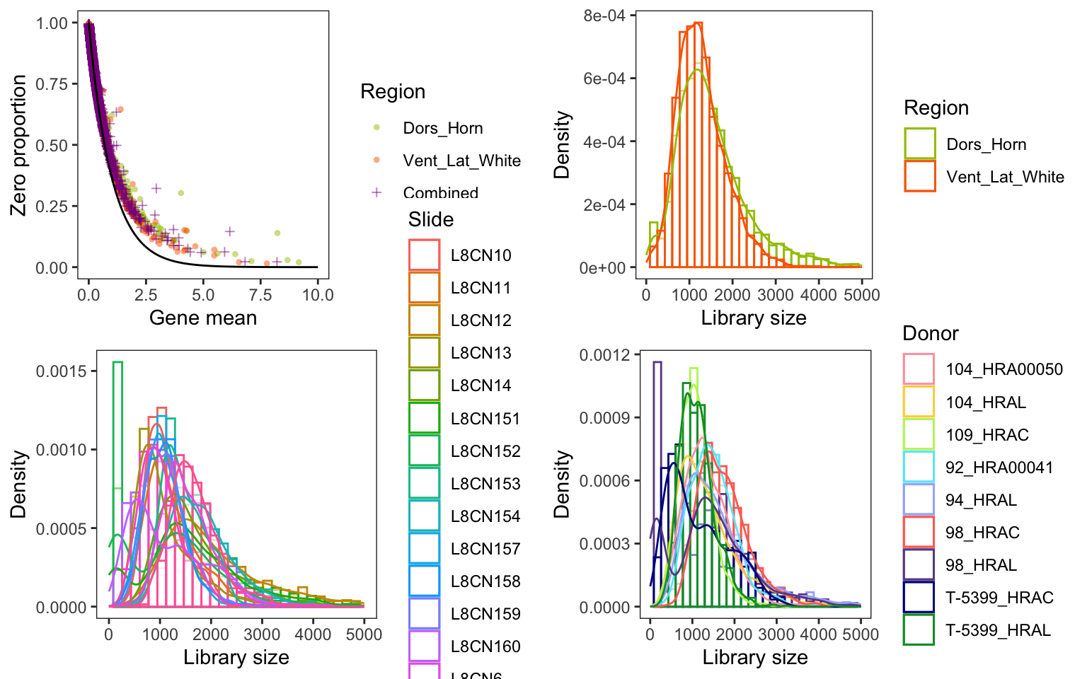

Difference in library size

ks_result = ks.test(subset(count_cell_df, Region == group1, totalcount)$totalcount, subset(count_cell_df, Region == group2, totalcount)$totalcount)

Warning in ks.test.default(subset(count_cell_df, Region == group1,
totalcount)$totalcount, : p-value will be approximate in the presence of ties

t_test = t.test(subset(count_cell_df, Region == group1, totalcount)$totalcount, subset(count_cell_df, Region == group2, totalcount)$totalcount)
print(ks_result)

    Asymptotic two-sample Kolmogorov-Smirnov test

data:  subset(count_cell_df, Region == group1, totalcount)$totalcount and subset(count_cell_df, Region == group2, totalcount)$totalcount
D = 0.12804, p-value < 2.2e-16
alternative hypothesis: two-sided

print(t_test)

    Welch Two Sample t-test

data:  subset(count_cell_df, Region == group1, totalcount)$totalcount and subset(count_cell_df, Region == group2, totalcount)$totalcount
t = 17.059, df = 7783.8, p-value < 2.2e-16
alternative hypothesis: true difference in means is not equal to 0
95 percent confidence interval:
 235.2685 296.3577
sample estimates:
mean of x mean of y 
 1549.826  1284.013 

Number of DEGs from each method

dflist = list(pois_glmm_df, 
              binom_glmm_df, 
              DESeq2.muscat,
              edgeR.cpm,
              MAST_donor_df, 
              Wilcox_Seurat_df,
              # MMdream,
              MMvst
              # MMpoisson
              )
titlelist = c("Poisson-glmm_UMI", 
              "Binomial-glmm_UMI",
              "pb-DESeq2_UMI", 
              "pb-edgeR_CPM",
              "MAST_CPM",
              "Wilcox_int",
              # "MMdream",
              "MMvst_VST"
              # "MMpoisson_UMI"
              )


number_input_hits = data.frame(DEGs = integer(0), Input = integer(0))
pois_glmm_inputgene = pois_glmm_df$genes[!is.na(pois_glmm_df$hits)]
for (df in dflist){
  number_input_hits = rbind(number_input_hits, 
                            c(sum(!is.na(df$hits)), 
                              sum(df$hits, na.rm = T))) 
}
colnames(number_input_hits) = c("Inputs", "DEGs")
number_input_hits$method = titlelist

number_input_hits = melt(number_input_hits, id = "method")
colnames(number_input_hits)[2:3] = c("Gene", "Number_of_genes")

# pdf("../submission preparation/graph_panels/panel4/input_hits.pdf", width = 8, height = 8)
ggplot(data=number_input_hits, aes(x=factor(method, 
                                            levels = titlelist), y=Number_of_genes, fill = Gene)) +
  geom_bar(stat="identity", position=position_dodge()) + 
  geom_text(aes(label=Number_of_genes), vjust=-0.2, position=position_dodge(0.9), size = 2) +
  theme_bw() + theme(panel.grid = element_blank()) +
  theme(axis.text.x = element_text(angle = 20, margin = margin(t = 15))) +
  scale_fill_manual(values = c("#BCAAA4", "#5D4037")) +
  xlab("") +
  ylab("Number of genes") +
  ggtitle(paste("DEGs summary"))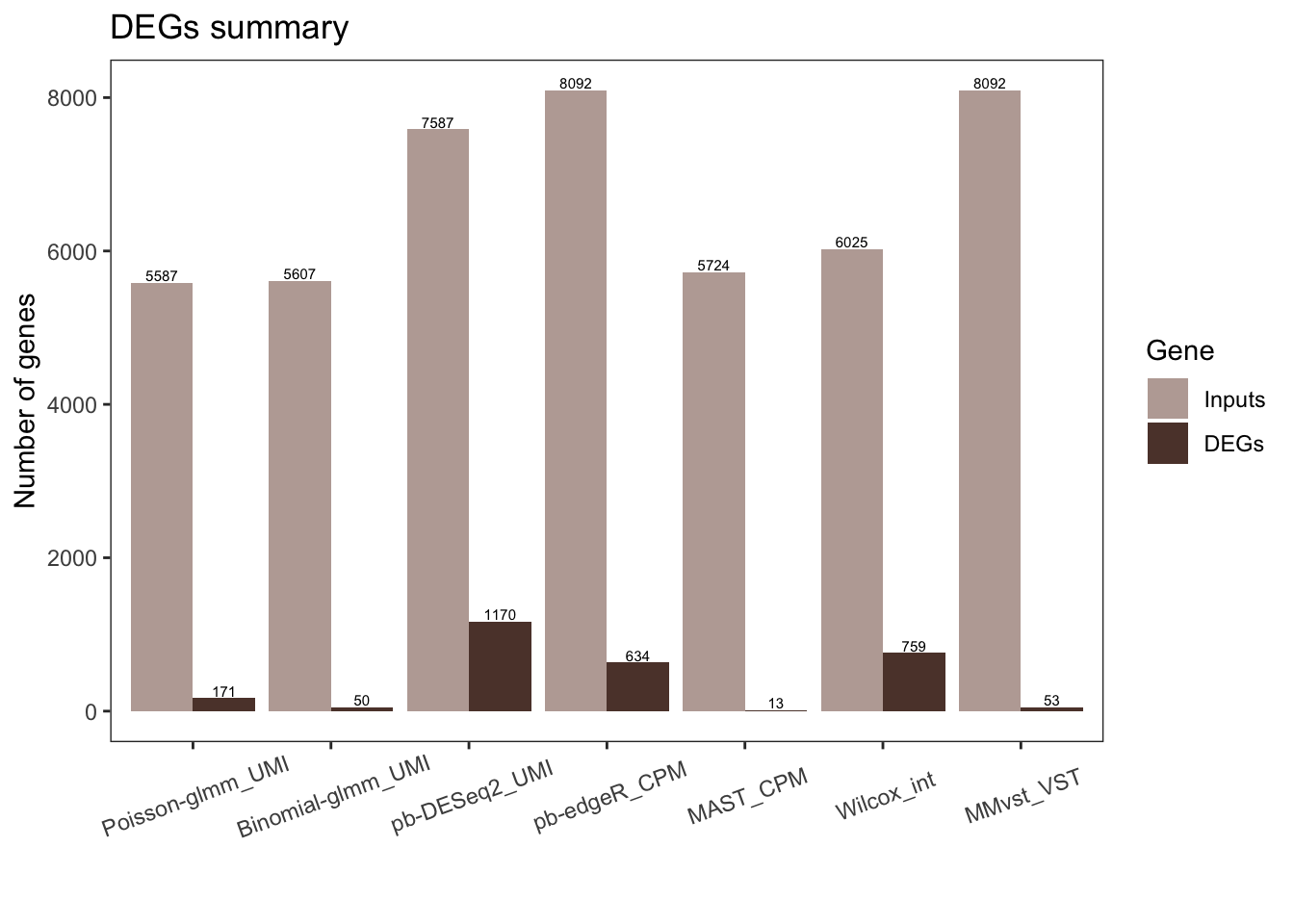

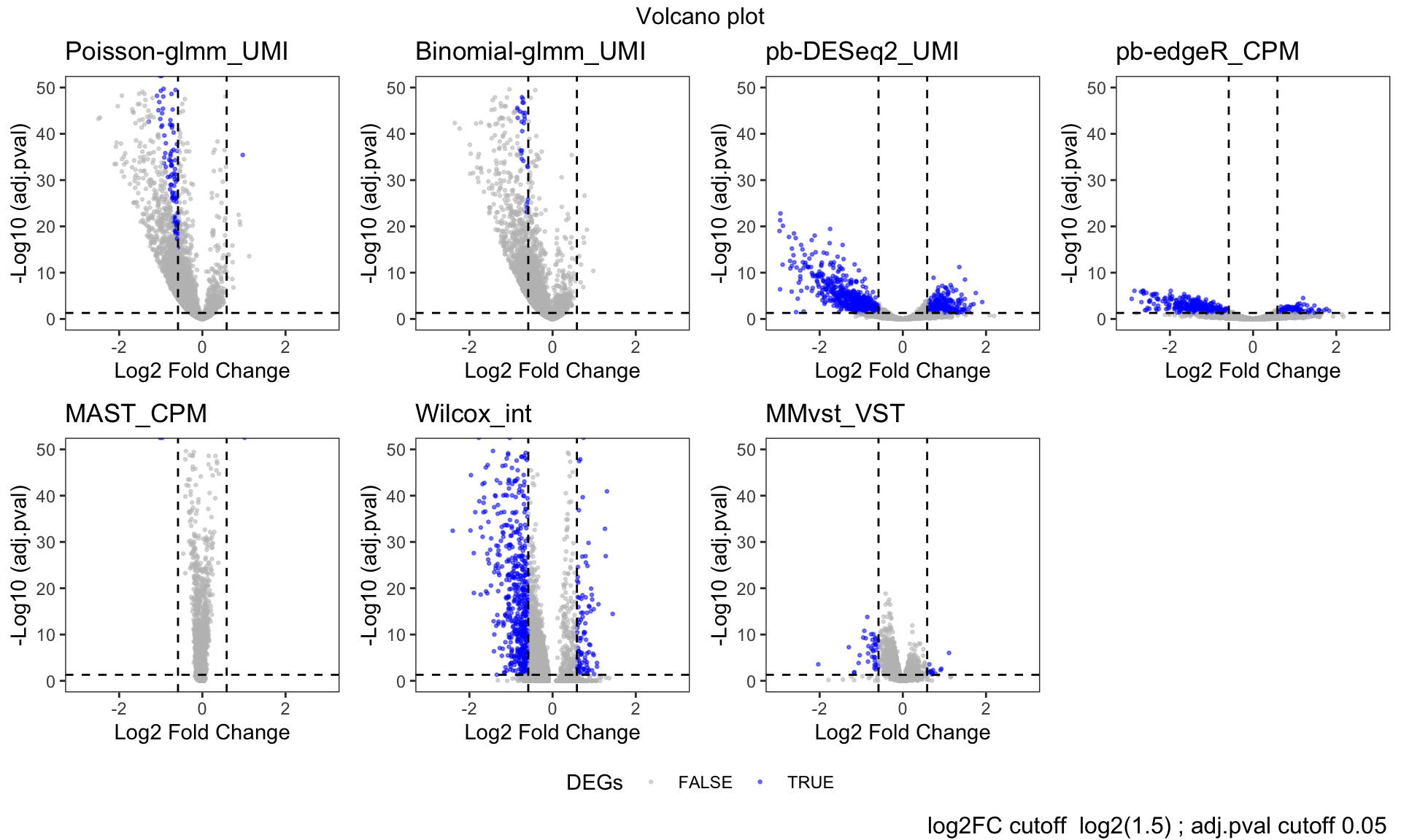
# dev.off()

Volcano plot

pvalcutoff = 0.05
v = 1.5
log2FCcutoff = log2(v)

p = list()
for (i in 1:length(dflist)){
  if(i %in% 6){
    xvar = 'avg_log2FC'
    yvar = 'p_val_adj'
  }else{
    xvar = 'log2FC'
    yvar = 'BH'
  }
  if (nrow(dflist[[i]])==0){next}
  p[[i]] = ggplot(na.omit(data.frame(dflist[[i]])), aes_string(x = xvar, y = sprintf("-log10(%s)", yvar), colour = "hits")) +
    geom_point(alpha = 0.5, size = 0.5) +
    labs(color = "hits") +
    geom_hline(yintercept=-log10(pvalcutoff),linetype=2) +
    geom_vline(xintercept=log2FCcutoff,linetype=2) + 
    geom_vline(xintercept=-log2FCcutoff,linetype=2) +
    ggtitle(titlelist[i]) + 
    theme_bw() + 
    theme(panel.grid = element_blank()) + 
    scale_color_manual(values = c("gray", "blue")) +
    labs(color = "DEGs") +
    xlim(c(-3,3)) + 
    ylim(c(0,50)) + 
    xlab("Log2 Fold Change") + 
    ylab("-Log10 (adj.pval)")
}

Warning: `aes_string()` was deprecated in ggplot2 3.0.0.
ℹ Please use tidy evaluation idioms with `aes()`.
ℹ See also `vignette("ggplot2-in-packages")` for more information.
This warning is displayed once every 8 hours.
Call `lifecycle::last_lifecycle_warnings()` to see where this warning was
generated.

figure = ggarrange(plotlist = p, common.legend = TRUE, legend="bottom", nrow = 2, ncol = 4)

Warning: Removed 121 rows containing missing values or values outside the scale range
(`geom_point()`).

Warning: Removed 121 rows containing missing values or values outside the scale range
(`geom_point()`).

Warning: Removed 55 rows containing missing values or values outside the scale range
(`geom_point()`).

Warning: Removed 8 rows containing missing values or values outside the scale range
(`geom_point()`).

Warning: Removed 6 rows containing missing values or values outside the scale range
(`geom_point()`).

Warning: Removed 56 rows containing missing values or values outside the scale range
(`geom_point()`).

Warning: Removed 122 rows containing missing values or values outside the scale range
(`geom_point()`).

# Annotate the figure by adding a common labels
annotate_figure(figure,
                top = paste("Volcano plot"),
                bottom = text_grob(paste( "log2FC cutoff ", paste0("log2(",v,")"),"; adj.pval cutoff", pvalcutoff)
                                   , x = 0.99, just = "right")
)

Histogram of p-value/adj.p-value

p = list()
for (i in 1:length(dflist)){
  if (nrow(dflist[[i]])==0){next}
  df = data.frame(genes = dflist[[i]]$genes)
  
  if(i %in% 6){
    df = cbind(df, dflist[[i]][,c("p_val", "p_val_adj")])
  }else{
    df = cbind(df, dflist[[i]][,c("pval", "BH")])
  }
  
  p[[i]] = ggplot(melt(df,id = "genes"), aes(x=value, color=variable)) +
geom_histogram(fill="white", alpha=0.5, position="identity") + theme_bw() + theme(panel.grid = element_blank()) + xlab(NULL) + ylab("Count") + 
coord_cartesian(ylim = c(0, 3000)) +
    ggtitle(titlelist[i]) + scale_colour_discrete(guide = guide_legend(title = NULL),labels = c("p-value", "adj.p-value"))
}
figure = ggarrange(plotlist = p, common.legend = TRUE, legend="bottom", nrow = 2, ncol = 4)

`stat_bin()` using `bins = 30`. Pick better value with `binwidth`.

Warning: Removed 5010 rows containing non-finite outside the scale range
(`stat_bin()`).

`stat_bin()` using `bins = 30`. Pick better value with `binwidth`.

Warning: Removed 5010 rows containing non-finite outside the scale range
(`stat_bin()`).

`stat_bin()` using `bins = 30`. Pick better value with `binwidth`.

Warning: Removed 4970 rows containing non-finite outside the scale range
(`stat_bin()`).

`stat_bin()` using `bins = 30`. Pick better value with `binwidth`.
`stat_bin()` using `bins = 30`. Pick better value with `binwidth`.
`stat_bin()` using `bins = 30`. Pick better value with `binwidth`.
`stat_bin()` using `bins = 30`. Pick better value with `binwidth`.
`stat_bin()` using `bins = 30`. Pick better value with `binwidth`.

annotate_figure(figure)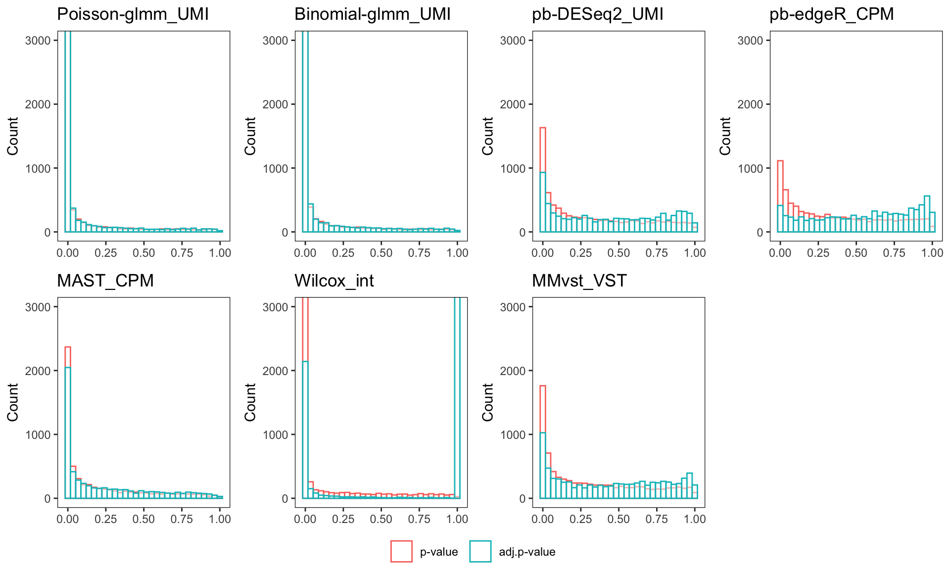

P-Value comparison across different methods

value = "pval"
p = list()
  for (i in 2:length(dflist)){
    if (nrow(dflist[[i]])==0){next}
    if (value == "pval"){
      xlimit = c(0,1)
      ylimit = c(0,1)
      if (is.null(dflist[[i]]$pval)){
        x = dflist[[i]]$p_val
      }else
        x = dflist[[i]]$pval
    }
    if (value == "log2FC"){
      xlimit = c(-3,3)
      ylimit = c(-3,3)
      if (is.null(dflist[[i]]$log2FC)){
        x = dflist[[i]]$avg_log2FC
      }else
        x = dflist[[i]]$log2FC
    }
    y = dflist[[1]][match(dflist[[i]]$genes, dflist[[1]]$genes),value]
    p[[i-1]] = ggplot(na.omit(data.frame(x = x, y = y)), aes(x = x, y = y)) +
      geom_point(alpha = 0.5, size = 0.5) + theme_minimal() + xlim(xlimit) + ylim(ylimit)+ 
      xlab(titlelist[i]) + ylab(titlelist[1])
  }
  figure = ggarrange(plotlist = p,nrow = 2, ncol = 4)
  
  # Annotate the figure by adding a common labels
  annotate_figure(figure,
                  top = paste(value, "comparison"))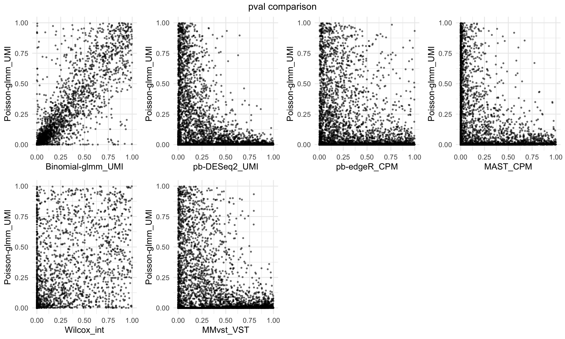

Log2 fold change comparison across different methods

value = "log2FC"
p = list()
  for (i in 2:length(dflist)){
    if (nrow(dflist[[i]])==0){next}
    if (value == "pval"){
      xlimit = c(0,1)
      ylimit = c(0,1)
      if (is.null(dflist[[i]]$pval)){
        x = dflist[[i]]$p_val
      }else
        x = dflist[[i]]$pval
    }
    if (value == "log2FC"){
      xlimit = c(-3,3)
      ylimit = c(-3,3)
      if (is.null(dflist[[i]]$log2FC)){
        x = dflist[[i]]$avg_log2FC
      }else
        x = dflist[[i]]$log2FC
    }
    y = dflist[[1]][match(dflist[[i]]$genes, dflist[[1]]$genes),value]
    p[[i-1]] = ggplot(na.omit(data.frame(x = x, y = y)), aes(x = x, y = y)) +
      geom_point(alpha = 0.5, size = 0.5) + theme_minimal() + xlim(xlimit) + ylim(ylimit)+ 
      xlab(titlelist[i]) + ylab(titlelist[1])
  }
  figure = ggarrange(plotlist = p,nrow = 2, ncol = 4)

Warning: Removed 2 rows containing missing values or values outside the scale range
(`geom_point()`).

Warning: Removed 5 rows containing missing values or values outside the scale range
(`geom_point()`).

Warning: Removed 4 rows containing missing values or values outside the scale range
(`geom_point()`).

Warning: Removed 2 rows containing missing values or values outside the scale range
(`geom_point()`).
Removed 2 rows containing missing values or values outside the scale range
(`geom_point()`).
Removed 2 rows containing missing values or values outside the scale range
(`geom_point()`).

  # Annotate the figure by adding a common labels
  annotate_figure(figure,
                  top = paste(value, "comparison"))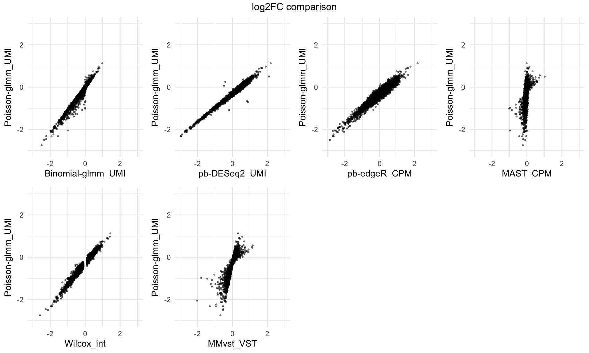

Violin plot of log2mean of DEGs

p = list()
df = data.frame()
clustername = pair
for (i in 1:length(dflist)){
  if (nrow(dflist[[i]])==0){next}
  if (sum(dflist[[i]]$hits, na.rm = T)==0){next}
  hits_gene = dflist[[i]]$genes[which(dflist[[i]]$hits)]
  if(length(hits_gene)>1){fun = rowMeans}else{fun = mean}
  for (j in 1:2){
    cellind = subgroupsce$region %in% clustername[j]
    df = rbind(df, data.frame(Log2mean = log2(fun(assays(subgroupsce)$counts[hits_gene,cellind])), Group = clustername[j], method = titlelist[i]))
  }
}

ggplot(df, aes(x = factor(method,levels = titlelist), y=Log2mean, fill = factor(Group))) +
  geom_violin() + 
  theme_bw() + 
  theme(panel.grid = element_blank()) + 
  ylim(c(-3,4)) + 
  xlab("") + 
  theme(axis.text.x = element_text(angle = 20, margin = margin(t = 15))) +
  labs(fill = "Region") +
  scale_fill_manual(values = region_palette[c(group1, group2)])

Warning: Removed 2993 rows containing non-finite outside the scale range
(`stat_ydensity()`).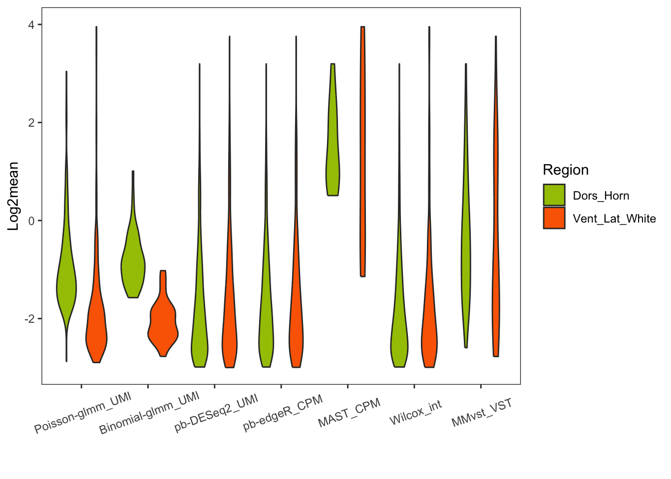

Violin plot of gene expression frequency of DEGs

p = list()
df = data.frame()
clusterlist = list(unique(sce_human_spine_filtered$region), group1, group2)
clustername = c("All region", group1, group2)
for (i in 1:length(dflist)){
  if (nrow(dflist[[i]])==0){next}
  if (sum(dflist[[i]]$hits, na.rm = T)==0){next}
  hits_gene = dflist[[i]]$genes[which(dflist[[i]]$hits)]

  if(length(hits_gene)>1){fun = rowMeans}else{fun = mean}
  for (j in 1:3){
    cellind = sce_human_spine_filtered$region %in% clusterlist[[j]]
    df = rbind(df, data.frame(freq = fun(assays(sce_human_spine_filtered)$counts[hits_gene,cellind]>0), cluster = clustername[j], method = titlelist[i]))
  }
}
levels(df$cluster) = clustername

ggplot(df, aes(x = factor(method,levels = titlelist), y=freq, fill = factor(cluster, levels =  levels(cluster)))) + 
  geom_violin() + 
  theme_bw() + 
  theme(panel.grid = element_blank()) + 
  ylab("Gene expression frequency") + 
  ylim(c(0,1)) + 
  xlab("") + 
  scale_fill_manual(values = c("All region" = "gray", region_palette[c(group1, group2)]), breaks = levels(df$cluster)) +
  labs(fill = "Region") +
  theme(axis.text.x = element_text(angle = 20, margin = margin(t = 15)))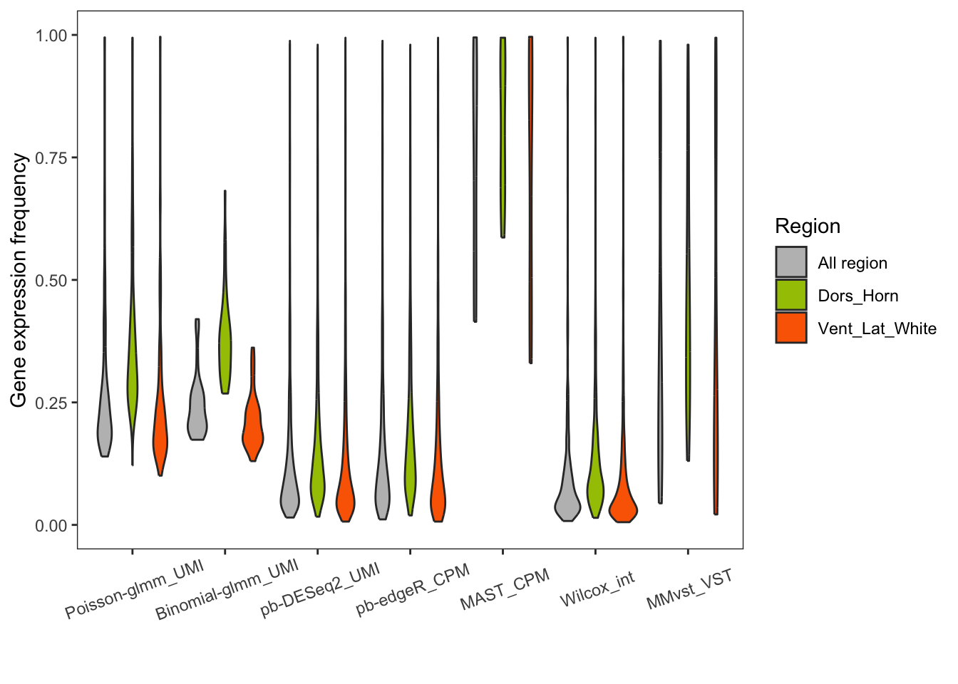 

Upset plot

library(UpSetR)
all_genes = c()
for(df in dflist){
  all_genes = c(all_genes, df$genes[which(df$hits)])
}

all_genes = unique(all_genes)

# Create a binary matrix where rows are genes and columns represent methods
upset_data = data.frame(gene = all_genes)
for (i in seq_along(dflist)){
  title = titlelist[i]
  upset_data[[title]] = as.numeric(all_genes %in% dflist[[i]]$genes[which(dflist[[i]]$hits)])
}

# Generate the upset plot
upset(upset_data[,-1], 
      sets = rev(titlelist), 
      keep.order = TRUE, 
      order.by = "freq")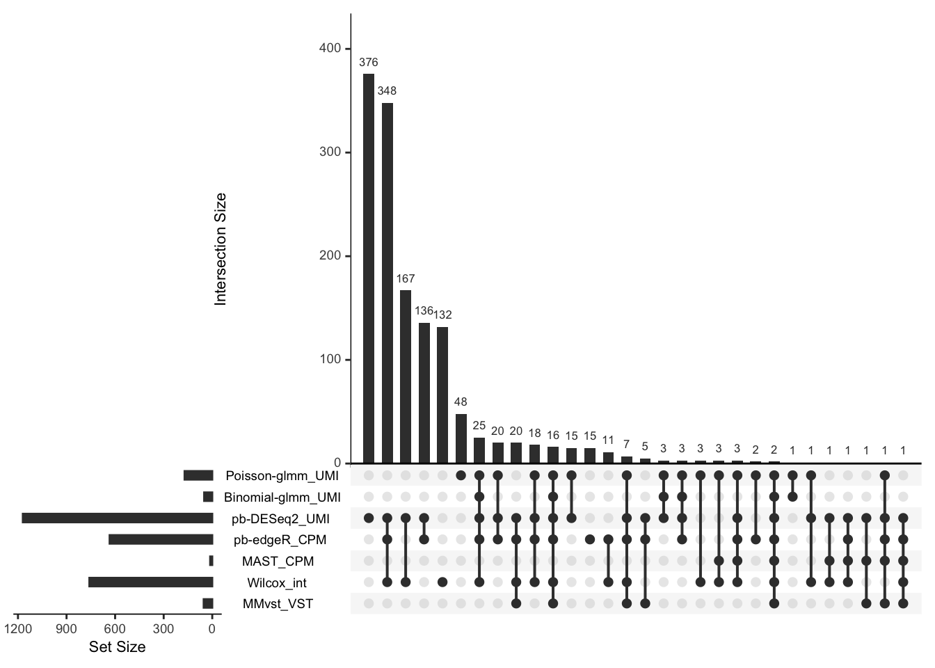

Heatmap of top DEGs

Poisson-glmm DEGs

sort_log2FC = sort(abs(pois_glmm_df$log2FC[pois_glmm_df$hits]), index.return = T, decreasing = T)
hitgenes = pois_glmm_df$genes[which(pois_glmm_df$hits)][sort_log2FC$ix]
mat = subgroupsce@assays@data$counts[hitgenes,]
#row annotation
annotation_log2FC = data.frame(abs_log2FC = abs(pois_glmm_df$log2FC[match(hitgenes,pois_glmm_df$genes)]))
rownames(annotation_log2FC) = rownames(mat)
#col annotation
annotation_df = data.frame(Donor = subgroupsce$patient_ID, Region = subgroupsce$region)
rownames(annotation_df) = colnames(mat)
annotation_df = annotation_df[with(annotation_df, order(Region, Donor)), ]
# cell level
pheatmap(mat[,rownames(annotation_df)],
         main = paste0("Poisson-glmm DEGs\nin UMI counts (", nrow(mat)," DEGs)"),
         annotation_col = annotation_df, 
         annotation_row = annotation_log2FC,
         annotation_colors = annotation_colors,
         cluster_rows=F, cluster_cols=F, 
         show_colnames = F, show_rownames = F,
         annotation_names_row = F,
         color=colorRampPalette(c("navy", "white", "red"))(10), breaks = seq(0,3, length.out = 10))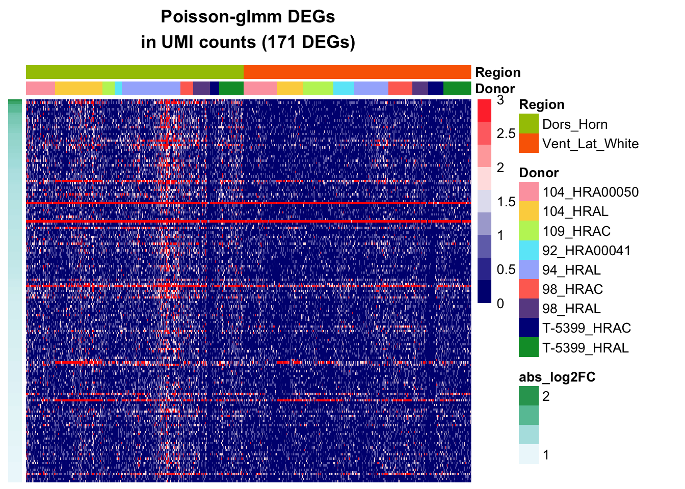

Additional DEGs from other methods

Wilcox

sort_log2FC = sort(abs(Wilcox_Seurat_df$avg_log2FC[Wilcox_Seurat_df$hits]), index.return = T, decreasing = T)
hitgenes_wilcox = Wilcox_Seurat_df$genes[which(Wilcox_Seurat_df$hits)][sort_log2FC$ix]
hits_notin_glmm = na.omit(hitgenes_wilcox[!hitgenes_wilcox%in%hitgenes])
mat = subgroupsce@assays@data$counts[hits_notin_glmm,]

# cell level
pheatmap(mat[,rownames(annotation_df)], 
         main = paste0("Wilcox DEGs \nnot identified by Poisson-glmm (",nrow(mat)," DEGs)"),
         annotation_col = annotation_df, 
         annotation_colors = annotation_colors,
         cluster_rows=F, cluster_cols=F, 
         show_colnames = F, show_rownames = F,
         annotation_names_row = F,
         color=colorRampPalette(c("navy", "white", "red"))(10), breaks = seq(0,3, length.out = 10))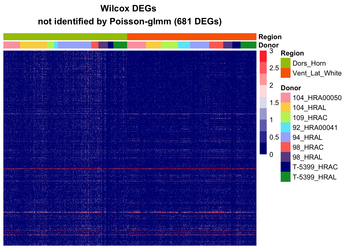

pb-DESeq2

sort_log2FC = sort(abs(DESeq2.muscat$log2FC[DESeq2.muscat$hits]), index.return = T, decreasing = T)
hitgenes_deseq2 = DESeq2.muscat$genes[which(DESeq2.muscat$hits)][sort_log2FC$ix]
hits_notin_glmm = na.omit(hitgenes_deseq2[!hitgenes_deseq2%in%hitgenes][1:600])
mat = subgroupsce@assays@data$counts[hits_notin_glmm,]

# cell level
pheatmap(mat[,rownames(annotation_df)], 
         main = paste0("pb-DESeq2 DEGs \nnot identified by Poisson-glmm (",nrow(mat)," DEGs)"),
         annotation_col = annotation_df, 
         annotation_colors = annotation_colors,
         cluster_rows=F, cluster_cols=F, 
         show_colnames = F, show_rownames = F,
         annotation_names_row = F,
         color=colorRampPalette(c("navy", "white", "red"))(10), breaks = seq(0,3, length.out = 10))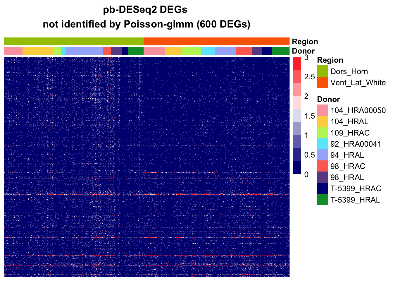

pdf("~/Google Drive/My Drive/spatial/10X/graph_panels/panel7/heatmap_deseq2.pdf", width = 5, height = 5)
pheatmap(mat[,rownames(annotation_df)], 
         main = paste0("pb-DESeq2 DEGs \nnot identified by Poisson-glmm (",nrow(mat)," DEGs)"),
         annotation_col = annotation_df, 
         annotation_row = annotation_log2FC,
         annotation_colors = annotation_colors,
         cluster_rows=F, cluster_cols=F, 
         show_colnames = F, show_rownames = F,
         annotation_names_row = F,
         color=colorRampPalette(c("navy", "white", "red"))(10), breaks = seq(0,3, length.out = 10))
dev.off()

MA plot

xvar = subgroupsce@metadata$log2mean
xlimits = c(-6,6)
xLabel = "Log2 mean"
p = list()
  for (i in 1:length(dflist)){
    if(is.null(dflist[[i]]$genes)){
      x = xvar[match(rownames(dflist[[i]]), names(xvar))]
    }else{
      x = xvar[match(dflist[[i]]$genes,names(xvar))]
    }
    if(is.null(dflist[[i]]$log2FC)){
      y = dflist[[i]]$avg_log2FC
    }else{
      y = dflist[[i]]$log2FC
    }
    p[[i]] = ggplot(na.omit(data.frame(x = x, y = y, DEGs = dflist[[i]]$hits)), aes(x = x, y = y, colour = DEGs)) +
      geom_point(alpha = 0.5, size = 0.5) +
      geom_hline(yintercept=log2(1.5),linetype=2) +
      geom_hline(yintercept=-log2(1.5),linetype=2) +
      ggtitle(titlelist[i]) + theme_minimal() + xlim(xlimits) + ylim(c(-4,4)) + 
      scale_color_manual(values = c("gray", "blue")) +
      xlab(xLabel) + ylab("Log2 Fold Change") + theme(legend.position = "bottom")
  }
  fig_FC_mean = ggarrange(plotlist = p,common.legend = TRUE, legend = "right", ncol = 4, nrow = 2)

Warning: Removed 2 rows containing missing values or values outside the scale range
(`geom_point()`).

Warning: Removed 176 rows containing missing values or values outside the scale range
(`geom_point()`).

Warning: Removed 134 rows containing missing values or values outside the scale range
(`geom_point()`).

Warning: Removed 175 rows containing missing values or values outside the scale range
(`geom_point()`).

  annotate_figure(fig_FC_mean, top = paste("Log2FC vs. Log2 mean "))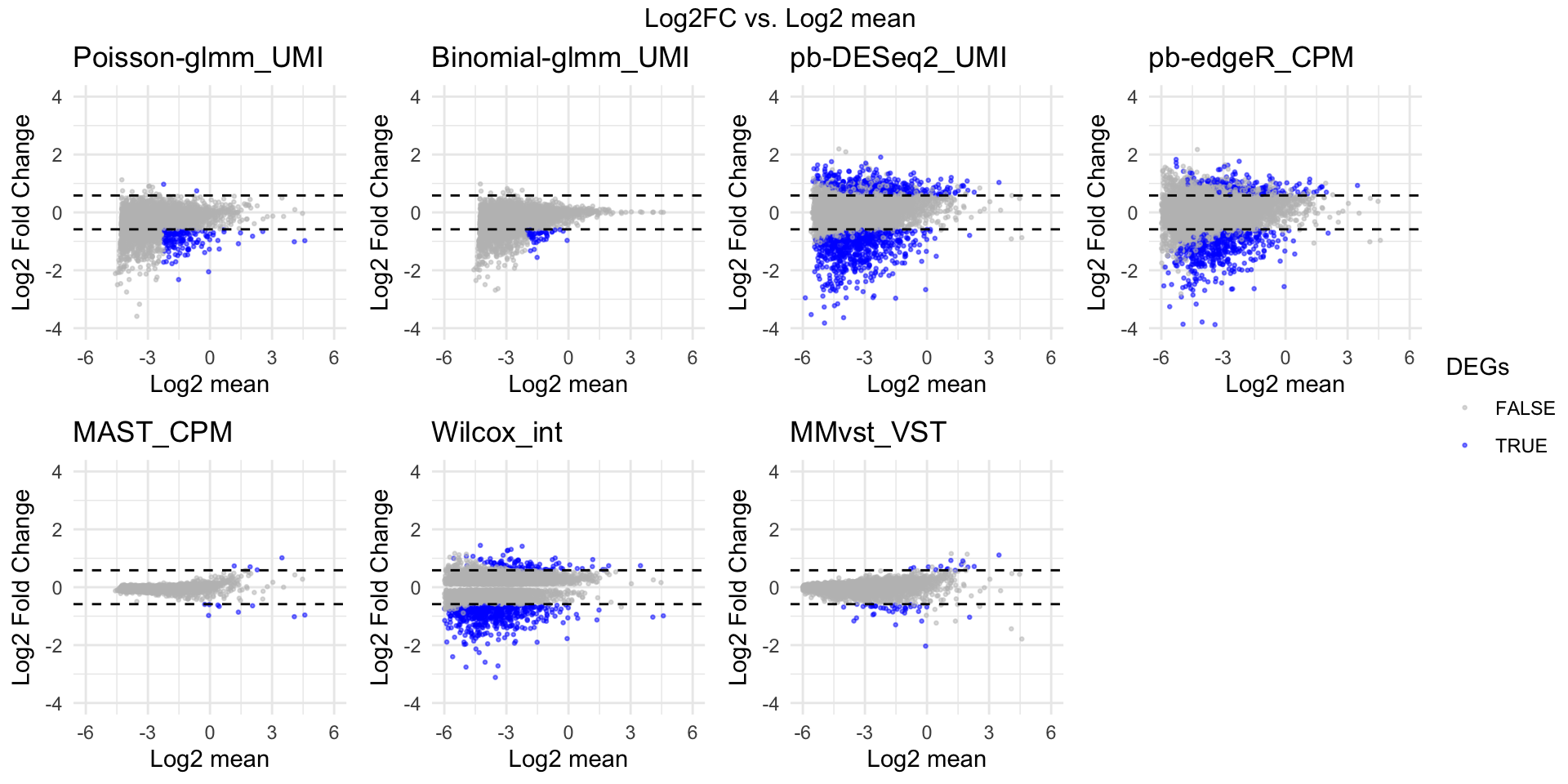

Enrichment analysis

GO object

original_gene_list = pois_glmm_df$log2FC
names(original_gene_list) = pois_glmm_df$genes
gene_list = na.omit(original_gene_list)
# sort the list in decreasing order (required for clusterProfiler)
gene_list = sort(gene_list, decreasing = TRUE)
genes = pois_glmm_df$genes[which(pois_glmm_df$hits)]
# create GO object
go_enrich = enrichGO(gene = genes,
                      universe = names(gene_list),
                      OrgDb = "org.Hs.eg.db", 
                      keyType = 'SYMBOL',
                      readable = T,
                      ont = "BP",
                      pvalueCutoff = 0.05, 
                      qvalueCutoff = 0.10)

dotplot(go_enrich)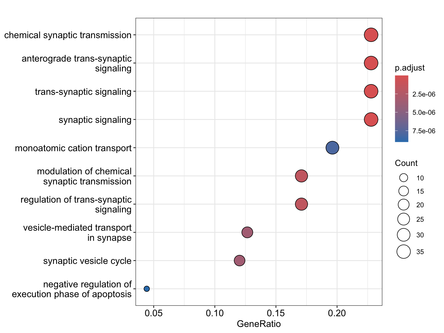

cnetplot(go_enrich, categorySize="pvalue", color.params = list(foldChange = gene_list))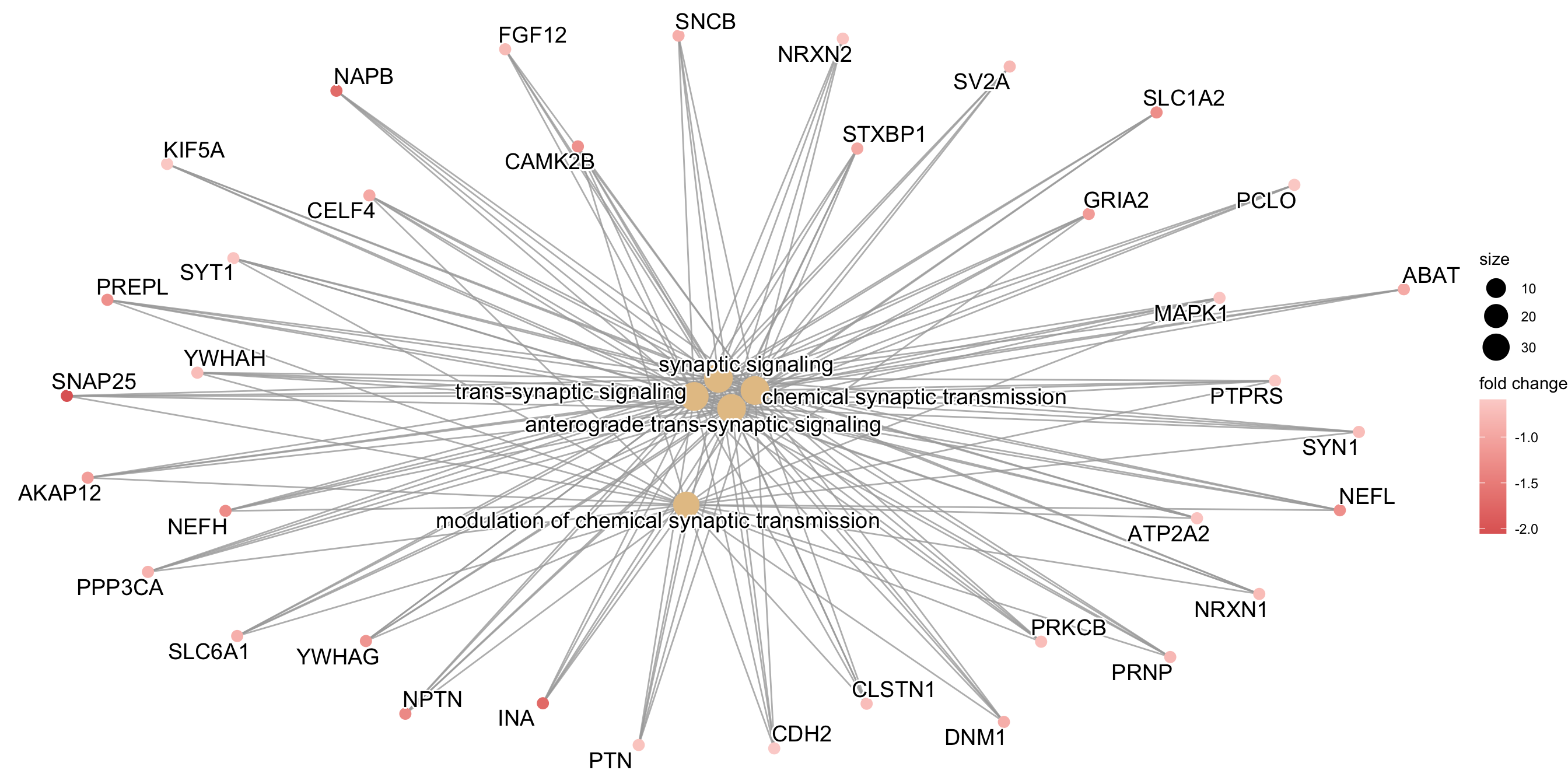

enrichKEGG object

# Convert gene IDs for enrichKEGG function
# We will lose some genes here because not all IDs will be converted
ids = bitr(names(original_gene_list), fromType = "SYMBOL", toType = "ENTREZID", OrgDb="org.Hs.eg.db") 

'select()' returned 1:1 mapping between keys and columns

Warning in bitr(names(original_gene_list), fromType = "SYMBOL", toType =
"ENTREZID", : 5.09% of input gene IDs are fail to map...

dedup_ids = ids[!duplicated(ids[c("SYMBOL")]),]

# Create a vector of the gene universe
match_logic = pois_glmm_df$genes %in% dedup_ids$SYMBOL
kegg_gene_list <- pois_glmm_df$log2FC[match_logic]
names(kegg_gene_list) <- dedup_ids$ENTREZID
kegg_gene_list<-na.omit(kegg_gene_list)
kegg_gene_list = sort(kegg_gene_list, decreasing = TRUE)
# hits
kegg_genes = na.omit(dedup_ids$ENTREZID[pois_glmm_df$hits[match_logic]])
# create enrichKEGG object
kk = enrichKEGG(gene=kegg_genes,
                universe=names(kegg_gene_list),
                organism="hsa", pvalueCutoff = 0.05, keyType = "ncbi-geneid")

Reading KEGG annotation online: "https://rest.kegg.jp/link/hsa/pathway"...

Reading KEGG annotation online: "https://rest.kegg.jp/list/pathway/hsa"...

Reading KEGG annotation online: "https://rest.kegg.jp/conv/ncbi-geneid/hsa"...

dotplot(kk, 
        showCategory = 10, 
        title = "Enriched Pathways",
        font.size = 8)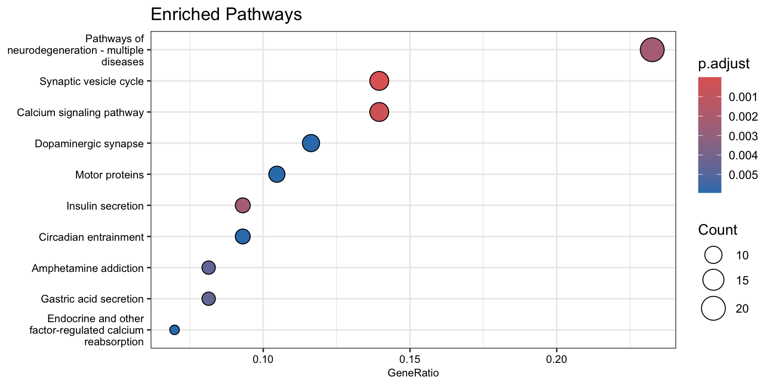

cnetplot(kk, categorySize="pvalue", foldChange=kegg_gene_list)

Warning in cnetplot.enrichResult(x, ...): Use 'color.params = list(foldChange = your_value)' instead of 'foldChange'.
 The foldChange parameter will be removed in the next version.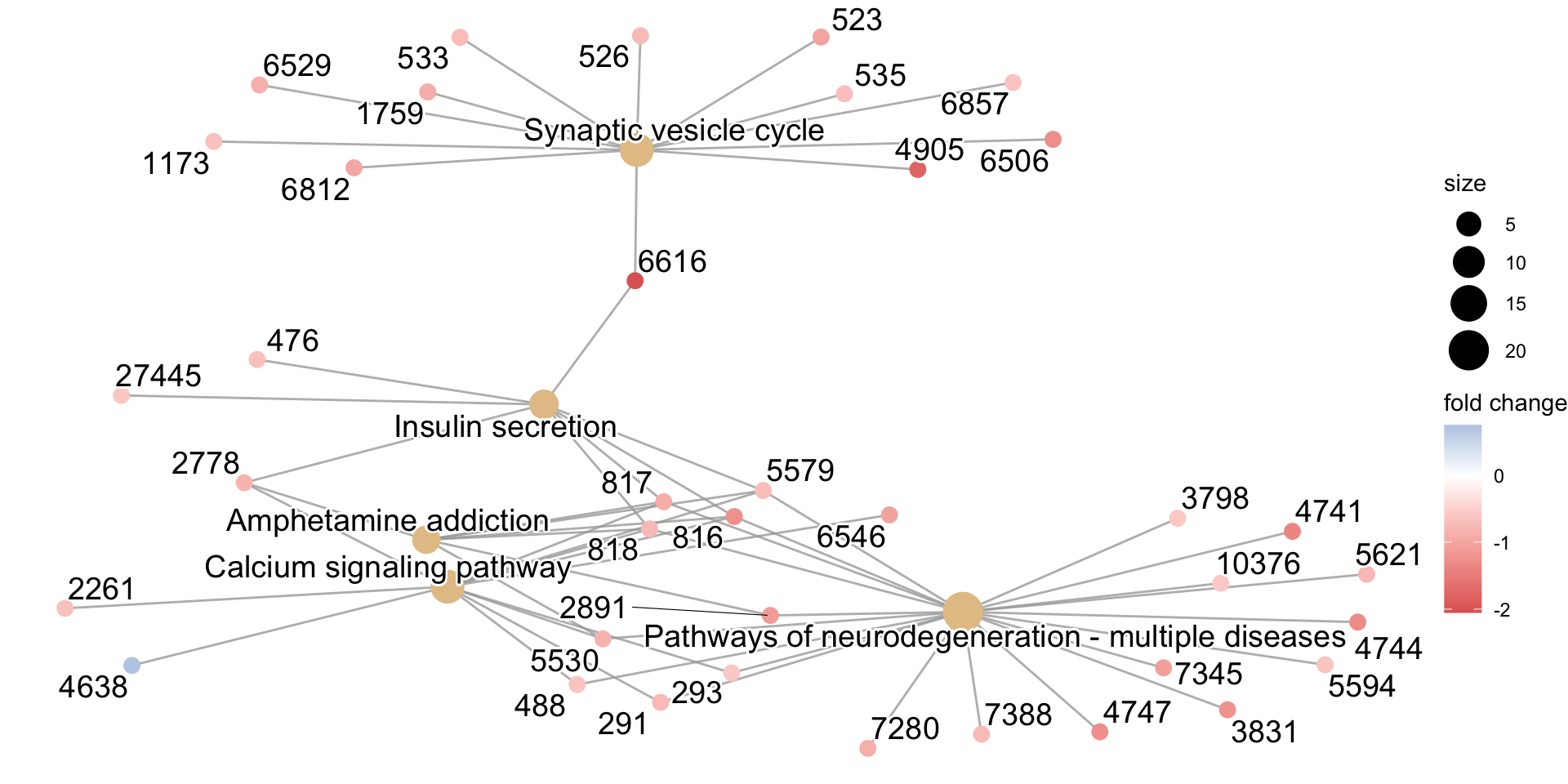

Session information

sessionInfo()

R version 4.4.1 (2024-06-14)
Platform: x86_64-apple-darwin20
Running under: macOS Monterey 12.6

Matrix products: default
BLAS:   /Library/Frameworks/R.framework/Versions/4.4-x86_64/Resources/lib/libRblas.0.dylib 
LAPACK: /Library/Frameworks/R.framework/Versions/4.4-x86_64/Resources/lib/libRlapack.dylib;  LAPACK version 3.12.0

locale:
[1] en_US.UTF-8/en_US.UTF-8/en_US.UTF-8/C/en_US.UTF-8/en_US.UTF-8

time zone: America/Chicago
tzcode source: internal

attached base packages:
[1] stats4    stats     graphics  grDevices utils     datasets  methods  
[8] base     

other attached packages:
 [1] UpSetR_1.4.0                pathview_1.44.0            
 [3] org.Hs.eg.db_3.19.1         AnnotationDbi_1.66.0       
 [5] enrichplot_1.24.4           clusterProfiler_4.12.6     
 [7] reshape_0.8.9               gridExtra_2.3              
 [9] pheatmap_1.0.12             SingleCellExperiment_1.26.0
[11] SummarizedExperiment_1.34.0 Biobase_2.64.0             
[13] GenomicRanges_1.56.2        GenomeInfoDb_1.40.1        
[15] IRanges_2.38.1              S4Vectors_0.42.1           
[17] BiocGenerics_0.50.0         MatrixGenerics_1.16.0      
[19] matrixStats_1.4.1           ggpubr_0.6.0               
[21] dplyr_1.1.4                 ggplot2_3.5.1              

loaded via a namespace (and not attached):
  [1] bitops_1.0-9            fs_1.6.4                spatstat.sparse_3.1-0  
  [4] httr_1.4.7              RColorBrewer_1.1-3      Rgraphviz_2.48.0       
  [7] tools_4.4.1             sctransform_0.4.1       backports_1.5.0        
 [10] utf8_1.2.4              R6_2.5.1                lazyeval_0.2.2         
 [13] uwot_0.2.2              withr_3.0.1             sp_2.1-4               
 [16] progressr_0.14.0        cli_3.6.3               spatstat.explore_3.3-2 
 [19] fastDummies_1.7.4       scatterpie_0.2.4        labeling_0.4.3         
 [22] sass_0.4.9              KEGGgraph_1.64.0        Seurat_5.1.0           
 [25] spatstat.data_3.1-2     ggridges_0.5.6          pbapply_1.7-2          
 [28] yulab.utils_0.1.7       gson_0.1.0              DOSE_3.30.5            
 [31] R.utils_2.12.3          parallelly_1.38.0       rstudioapi_0.16.0      
 [34] RSQLite_2.3.7           generics_0.1.3          gridGraphics_0.5-1     
 [37] ica_1.0-3               spatstat.random_3.3-2   car_3.1-3              
 [40] GO.db_3.19.1            Matrix_1.7-0            fansi_1.0.6            
 [43] abind_1.4-8             R.methodsS3_1.8.2       lifecycle_1.0.4        
 [46] whisker_0.4.1           yaml_2.3.10             carData_3.0-5          
 [49] qvalue_2.36.0           SparseArray_1.4.8       Rtsne_0.17             
 [52] grid_4.4.1              blob_1.2.4              promises_1.3.0         
 [55] crayon_1.5.3            miniUI_0.1.1.1          lattice_0.22-6         
 [58] cowplot_1.1.3           KEGGREST_1.44.1         pillar_1.9.0           
 [61] knitr_1.48              fgsea_1.30.0            future.apply_1.11.2    
 [64] codetools_0.2-20        fastmatch_1.1-4         leiden_0.4.3.1         
 [67] glue_1.8.0              ggfun_0.1.6             spatstat.univar_3.0-1  
 [70] data.table_1.16.2       vctrs_0.6.5             png_0.1-8              
 [73] treeio_1.28.0           spam_2.11-0             gtable_0.3.5           
 [76] cachem_1.1.0            xfun_0.48               S4Arrays_1.4.1         
 [79] mime_0.12               tidygraph_1.3.1         survival_3.7-0         
 [82] fitdistrplus_1.2-1      ROCR_1.0-11             nlme_3.1-166           
 [85] ggtree_3.12.0           bit64_4.5.2             RcppAnnoy_0.0.22       
 [88] rprojroot_2.0.4         bslib_0.8.0             irlba_2.3.5.1          
 [91] KernSmooth_2.23-24      colorspace_2.1-1        DBI_1.2.3              
 [94] tidyselect_1.2.1        bit_4.5.0               compiler_4.4.1         
 [97] git2r_0.33.0            graph_1.82.0            httr2_1.0.5            
[100] DelayedArray_0.30.1     plotly_4.10.4           shadowtext_0.1.4       
[103] scales_1.3.0            lmtest_0.9-40           rappdirs_0.3.3         
[106] stringr_1.5.1           digest_0.6.37           goftest_1.2-3          
[109] spatstat.utils_3.1-0    rmarkdown_2.28          XVector_0.44.0         
[112] htmltools_0.5.8.1       pkgconfig_2.0.3         highr_0.11             
[115] fastmap_1.2.0           rlang_1.1.4             htmlwidgets_1.6.4      
[118] UCSC.utils_1.0.0        shiny_1.9.1             farver_2.1.2           
[121] jquerylib_0.1.4         zoo_1.8-12              jsonlite_1.8.9         
[124] BiocParallel_1.38.0     GOSemSim_2.30.2         R.oo_1.26.0            
[127] RCurl_1.98-1.16         magrittr_2.0.3          Formula_1.2-5          
[130] GenomeInfoDbData_1.2.12 ggplotify_0.1.2         dotCall64_1.2          
[133] patchwork_1.3.0         munsell_0.5.1           Rcpp_1.0.13            
[136] ggnewscale_0.5.0        ape_5.8                 viridis_0.6.5          
[139] reticulate_1.39.0       stringi_1.8.4           ggraph_2.2.1           
[142] zlibbioc_1.50.0         MASS_7.3-61             plyr_1.8.9             
[145] parallel_4.4.1          listenv_0.9.1           ggrepel_0.9.6          
[148] deldir_2.0-4            Biostrings_2.72.1       graphlayouts_1.2.0     
[151] splines_4.4.1           tensor_1.5              igraph_2.0.3           
[154] spatstat.geom_3.3-3     ggsignif_0.6.4          RcppHNSW_0.6.0         
[157] reshape2_1.4.4          XML_3.99-0.17           evaluate_1.0.1         
[160] SeuratObject_5.0.2      tweenr_2.0.3            httpuv_1.6.15          
[163] RANN_2.6.2              tidyr_1.3.1             purrr_1.0.2            
[166] polyclip_1.10-7         future_1.34.0           scattermore_1.2        
[169] ggforce_0.4.2           broom_1.0.7             xtable_1.8-4           
[172] RSpectra_0.16-2         tidytree_0.4.6          rstatix_0.7.2          
[175] later_1.3.2             viridisLite_0.4.2       tibble_3.2.1           
[178] aplot_0.2.3             memoise_2.0.1           cluster_2.1.6          
[181] workflowr_1.7.1         globals_0.16.3