Trend Filtering Examples

Last updated: 2019-11-08

Checks: 7 0

Knit directory: SMF/

This reproducible R Markdown analysis was created with workflowr (version 1.5.0). The Checks tab describes the reproducibility checks that were applied when the results were created. The Past versions tab lists the development history.

R Markdown file: up-to-date

Great! Since the R Markdown file has been committed to the Git repository, you know the exact version of the code that produced these results.

Environment: empty

Great job! The global environment was empty. Objects defined in the global environment can affect the analysis in your R Markdown file in unknown ways. For reproduciblity it’s best to always run the code in an empty environment.

Seed: set.seed(20190719)

The command set.seed(20190719) was run prior to running the code in the R Markdown file. Setting a seed ensures that any results that rely on randomness, e.g. subsampling or permutations, are reproducible.

Session information: recorded

Great job! Recording the operating system, R version, and package versions is critical for reproducibility.

Cache: none

Nice! There were no cached chunks for this analysis, so you can be confident that you successfully produced the results during this run.

File paths: relative

Great job! Using relative paths to the files within your workflowr project makes it easier to run your code on other machines.

Repository version: f12ab55

Great! You are using Git for version control. Tracking code development and connecting the code version to the results is critical for reproducibility. The version displayed above was the version of the Git repository at the time these results were generated.

Note that you need to be careful to ensure that all relevant files for the analysis have been committed to Git prior to generating the results (you can use wflow_publish or wflow_git_commit). workflowr only checks the R Markdown file, but you know if there are other scripts or data files that it depends on. Below is the status of the Git repository when the results were generated:


Ignored files:
    Ignored:    .DS_Store
    Ignored:    .Rhistory
    Ignored:    .Rproj.user/
    Ignored:    analysis/.DS_Store

Unstaged changes:
    Modified:   analysis/index.Rmd
    Modified:   analysis/poissonmeanscale.Rmd

Note that any generated files, e.g. HTML, png, CSS, etc., are not included in this status report because it is ok for generated content to have uncommitted changes.

These are the previous versions of the R Markdown and HTML files. If you’ve configured a remote Git repository (see ?wflow_git_remote), click on the hyperlinks in the table below to view them.

File	Version	Author	Date	Message
Rmd	f12ab55	Dongyue Xie	2019-11-08	wflow_publish(“analysis/tfexample.Rmd”)

Introduction

Normal likelihood: Trend filtering from genlasso, glmgen, lasso form fitted using glmnet, susie-trendfiltering, Bayesian trend filtering from btf, spmrf.

Poisson likelihood: glmgen, spmrf, likelihood expansion, VST.

Normal likelihood

library(genlasso)

Loading required package: MASS

Loading required package: Matrix

Loading required package: igraph


Attaching package: 'igraph'

The following objects are masked from 'package:stats':

    decompose, spectrum

The following object is masked from 'package:base':

    union

library(glmgen)


Attaching package: 'glmgen'

The following object is masked from 'package:genlasso':

    trendfilter

library(glmnet)

Loading required package: foreach

Loaded glmnet 2.0-18

library(susieR)
library(btf)
library(spmrf)
library(rstan)

Loading required package: StanHeaders

Loading required package: ggplot2

rstan (Version 2.19.2, GitRev: 2e1f913d3ca3)

For execution on a local, multicore CPU with excess RAM we recommend calling
options(mc.cores = parallel::detectCores()).
To avoid recompilation of unchanged Stan programs, we recommend calling
rstan_options(auto_write = TRUE)

GenH = function(n,k){
  H = matrix(nrow=n,ncol=n)
  for(i in 1:n){
    for(j in 1:(k+1)){
      H[i,j] = i^(j-1)/n^(j-1)
    }
  }
  for(j in (k+2):n){
    for(i in 1:(j-1)){
      H[i,j] = 0
    }
    sigmak = Kcusum(n,j,k)
    for(i in j:n){
      H[i,j] = sigmak[i-j+1]*factorial(k)/n^k
    }
  }
  H
  
}

Kcusum = function(n,j,k){
  sigma = rep(1,n-j+1)
  if(k==0){
    return(rep(1,n-j+1))
  }else{
    for(t in 1:k){
      sigma = cumsum(sigma)
    }
    return(sigma)
  }
  
}

TF_lasso = function(y,k){
  n = length(y)
  H = GenH(n,k)
  fit = cv.glmnet(H,y,penalty.factor = c(rep(0,k+1),rep(1,n-k-1)),intercept = F,standardize=F)
  H%*%coef(fit,s='lambda.min')[-1]
}

Generate date from \(y = f + \epsilon\), \(\epsilon\sim N(0,\sigma^2)\). SNR = 1

Step function.

n = 100
x = (1:n)/n
sigma = 1
f = c(rep(3,n/4),rep(5,n/4),rep(8,n/4),rep(4,n/4))
snr = 1
f = f/sqrt(var(f)/sigma^2/snr)
y = f + rnorm(n,0,sigma)

#trend filtering
t1_tf=Sys.time()
fit_tf = genlasso::trendfilter(y,ord=0)
fit_tf_cv = cv.trendfilter(fit_tf)

Fold 1 ... Fold 2 ... Fold 3 ... Fold 4 ... Fold 5 ...

fit_tf = fit_tf$beta[,fit_tf$lambda==fit_tf_cv$lambda.min]
t2_tf=Sys.time()
#lasso form 
t1_lasso=Sys.time()
fit_lasso = TF_lasso(y,0)
t2_lasso=Sys.time()
#susie
t1_susie=Sys.time()
fit_susie = susie_trendfilter(y,0)
t2_susie=Sys.time()
#btf
t1_btf=Sys.time()
fit_btf = btf(y,k=0)
t2_btf=Sys.time()
#spmrf
t1_spmrf=Sys.time()
spmrf_obj = spmrf(data=list(y=y),prior="horseshoe", likelihood="normal", order=1,zeta=0.01,chains=0)

the number of chains is less than 1; sampling not done

nchain <- 2
ntotsamp <- 1000
nthin <- 1
nburn <- 500
niter <- (ntotsamp/nchain)*nthin + nburn
pars.H <- c("theta", "tau", "gam", "sigma") 
spmrf_draw = spmrf(prior="horseshoe", likelihood="normal", order=1,  fit=spmrf_obj,data=list(y=y),
                  par=pars.H, chains=nchain, warmup=nburn, thin=nthin, iter=niter,
                            control=list(adapt_delta=0.995, max_treedepth=12))


SAMPLING FOR MODEL 'horseshoe_normal_1' NOW (CHAIN 1).
Chain 1: 
Chain 1: Gradient evaluation took 8.1e-05 seconds
Chain 1: 1000 transitions using 10 leapfrog steps per transition would take 0.81 seconds.
Chain 1: Adjust your expectations accordingly!
Chain 1: 
Chain 1: 
Chain 1: Iteration:   1 / 1000 [  0%]  (Warmup)
Chain 1: Iteration: 100 / 1000 [ 10%]  (Warmup)
Chain 1: Iteration: 200 / 1000 [ 20%]  (Warmup)
Chain 1: Iteration: 300 / 1000 [ 30%]  (Warmup)
Chain 1: Iteration: 400 / 1000 [ 40%]  (Warmup)
Chain 1: Iteration: 500 / 1000 [ 50%]  (Warmup)
Chain 1: Iteration: 501 / 1000 [ 50%]  (Sampling)
Chain 1: Iteration: 600 / 1000 [ 60%]  (Sampling)
Chain 1: Iteration: 700 / 1000 [ 70%]  (Sampling)
Chain 1: Iteration: 800 / 1000 [ 80%]  (Sampling)
Chain 1: Iteration: 900 / 1000 [ 90%]  (Sampling)
Chain 1: Iteration: 1000 / 1000 [100%]  (Sampling)
Chain 1: 
Chain 1:  Elapsed Time: 12.3621 seconds (Warm-up)
Chain 1:                13.2683 seconds (Sampling)
Chain 1:                25.6305 seconds (Total)
Chain 1: 

SAMPLING FOR MODEL 'horseshoe_normal_1' NOW (CHAIN 2).
Chain 2: 
Chain 2: Gradient evaluation took 3.6e-05 seconds
Chain 2: 1000 transitions using 10 leapfrog steps per transition would take 0.36 seconds.
Chain 2: Adjust your expectations accordingly!
Chain 2: 
Chain 2: 
Chain 2: Iteration:   1 / 1000 [  0%]  (Warmup)
Chain 2: Iteration: 100 / 1000 [ 10%]  (Warmup)
Chain 2: Iteration: 200 / 1000 [ 20%]  (Warmup)
Chain 2: Iteration: 300 / 1000 [ 30%]  (Warmup)
Chain 2: Iteration: 400 / 1000 [ 40%]  (Warmup)
Chain 2: Iteration: 500 / 1000 [ 50%]  (Warmup)
Chain 2: Iteration: 501 / 1000 [ 50%]  (Sampling)
Chain 2: Iteration: 600 / 1000 [ 60%]  (Sampling)
Chain 2: Iteration: 700 / 1000 [ 70%]  (Sampling)
Chain 2: Iteration: 800 / 1000 [ 80%]  (Sampling)
Chain 2: Iteration: 900 / 1000 [ 90%]  (Sampling)
Chain 2: Iteration: 1000 / 1000 [100%]  (Sampling)
Chain 2: 
Chain 2:  Elapsed Time: 13.2592 seconds (Warm-up)
Chain 2:                13.3923 seconds (Sampling)
Chain 2:                26.6515 seconds (Total)
Chain 2:

Warning: There were 1 divergent transitions after warmup. Increasing adapt_delta above 0.995 may help. See
http://mc-stan.org/misc/warnings.html#divergent-transitions-after-warmup

Warning: Examine the pairs() plot to diagnose sampling problems

#fit_spmrf = as.array(spmrf_draw)
fit_spmrf_ci = extract_theta(spmrf_draw,obstype = 'normal',alpha=0.05)
fit_spmrf = fit_spmrf_ci$postmed
t2_spmrf=Sys.time()


plot(y,col = 'grey80')
lines(f,col='grey80')
lines(fit_tf,col=1)
lines(c(fit_lasso),col=2)
lines(fit_susie$fitted,col=3)
lines(apply(fit_btf$f,2,mean),col=4)
lines(fit_spmrf,col=7)
legend('topleft',c('truth','tf','lasso tf','susie','btf','spmrf'),lty=c(1,1,1,1,1,1),col=c('grey80',1,2,3,4,7))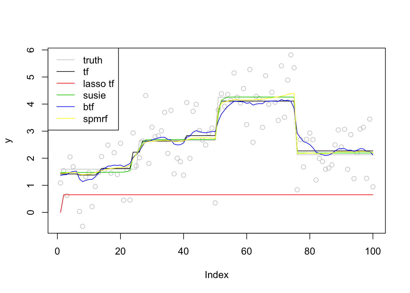

run time

paste0('tf run time:',round(t2_tf-t1_tf,2))

[1] "tf run time:0.77"

paste0('tf_lasso run time:',round(t2_lasso-t1_lasso,2))

[1] "tf_lasso run time:0.1"

paste0('susie run time:',round(t2_susie-t1_susie,2))

[1] "susie run time:0.1"

paste0('btf run time:',round(t2_btf-t1_btf,2))

[1] "btf run time:6.08"

paste0('spmrf run time:',round(t2_spmrf-t1_spmrf,2))

[1] "spmrf run time:1.54"

Poisson likelihood

n = 200
x = (1:n)/n
f = c(rep(2,n/4),rep(5,n/4),rep(8,n/4),rep(3,n/4))
y = rpois(n,f)

#trend filtering
t1_tf=Sys.time()
fit_tf = glmgen::trendfilter(x,y,k=0,family = 'poisson')
t2_tf=Sys.time()
# #lasso form 
# t1_lasso=Sys.time()
# fit_lasso = TF_lasso(y,0)
# t2_lasso=Sys.time()
# #susie
# t1_susie=Sys.time()
# fit_susie = susie_trendfilter(y,0)
# t2_susie=Sys.time()
# #btf
# t1_btf=Sys.time()
# fit_btf = btf(y,k=0)
# t2_btf=Sys.time()
#spmrf
t1_spmrf=Sys.time()
spmrf_obj = spmrf(data=list(y=y),prior="horseshoe", likelihood="poisson",order=1,zeta=0.01,chains=0)

the number of chains is less than 1; sampling not done

nchain <- 2
ntotsamp <- 1000
nthin <- 1
nburn <- 500
niter <- (ntotsamp/nchain)*nthin + nburn
pars.H <- c("theta", "tau", "gam") 
spmrf_draw = spmrf(prior="horseshoe", likelihood="poisson", order=1,  fit=spmrf_obj,data=list(y=y),
                  par=pars.H, chains=nchain, warmup=nburn, thin=nthin, iter=niter,
                            control=list(adapt_delta=0.995, max_treedepth=12))


SAMPLING FOR MODEL 'horseshoe_poisson_1' NOW (CHAIN 1).
Chain 1: 
Chain 1: Gradient evaluation took 8.3e-05 seconds
Chain 1: 1000 transitions using 10 leapfrog steps per transition would take 0.83 seconds.
Chain 1: Adjust your expectations accordingly!
Chain 1: 
Chain 1: 
Chain 1: Iteration:   1 / 1000 [  0%]  (Warmup)
Chain 1: Iteration: 100 / 1000 [ 10%]  (Warmup)
Chain 1: Iteration: 200 / 1000 [ 20%]  (Warmup)
Chain 1: Iteration: 300 / 1000 [ 30%]  (Warmup)
Chain 1: Iteration: 400 / 1000 [ 40%]  (Warmup)
Chain 1: Iteration: 500 / 1000 [ 50%]  (Warmup)
Chain 1: Iteration: 501 / 1000 [ 50%]  (Sampling)
Chain 1: Iteration: 600 / 1000 [ 60%]  (Sampling)
Chain 1: Iteration: 700 / 1000 [ 70%]  (Sampling)
Chain 1: Iteration: 800 / 1000 [ 80%]  (Sampling)
Chain 1: Iteration: 900 / 1000 [ 90%]  (Sampling)
Chain 1: Iteration: 1000 / 1000 [100%]  (Sampling)
Chain 1: 
Chain 1:  Elapsed Time: 41.7724 seconds (Warm-up)
Chain 1:                53.7048 seconds (Sampling)
Chain 1:                95.4772 seconds (Total)
Chain 1: 

SAMPLING FOR MODEL 'horseshoe_poisson_1' NOW (CHAIN 2).
Chain 2: 
Chain 2: Gradient evaluation took 7.3e-05 seconds
Chain 2: 1000 transitions using 10 leapfrog steps per transition would take 0.73 seconds.
Chain 2: Adjust your expectations accordingly!
Chain 2: 
Chain 2: 
Chain 2: Iteration:   1 / 1000 [  0%]  (Warmup)
Chain 2: Iteration: 100 / 1000 [ 10%]  (Warmup)
Chain 2: Iteration: 200 / 1000 [ 20%]  (Warmup)
Chain 2: Iteration: 300 / 1000 [ 30%]  (Warmup)
Chain 2: Iteration: 400 / 1000 [ 40%]  (Warmup)
Chain 2: Iteration: 500 / 1000 [ 50%]  (Warmup)
Chain 2: Iteration: 501 / 1000 [ 50%]  (Sampling)
Chain 2: Iteration: 600 / 1000 [ 60%]  (Sampling)
Chain 2: Iteration: 700 / 1000 [ 70%]  (Sampling)
Chain 2: Iteration: 800 / 1000 [ 80%]  (Sampling)
Chain 2: Iteration: 900 / 1000 [ 90%]  (Sampling)
Chain 2: Iteration: 1000 / 1000 [100%]  (Sampling)
Chain 2: 
Chain 2:  Elapsed Time: 39.6983 seconds (Warm-up)
Chain 2:                25.3519 seconds (Sampling)
Chain 2:                65.0502 seconds (Total)
Chain 2:

Warning: There were 3 divergent transitions after warmup. Increasing adapt_delta above 0.995 may help. See
http://mc-stan.org/misc/warnings.html#divergent-transitions-after-warmup

Warning: Examine the pairs() plot to diagnose sampling problems

Warning: Bulk Effective Samples Size (ESS) is too low, indicating posterior means and medians may be unreliable.
Running the chains for more iterations may help. See
http://mc-stan.org/misc/warnings.html#bulk-ess

#fit_spmrf = as.array(spmrf_draw)
fit_spmrf_ci = extract_theta(spmrf_draw,obstype = 'poisson',alpha=0.05)
fit_spmrf = fit_spmrf_ci$postmed
t2_spmrf=Sys.time()


plot(y,col = 'grey80')
lines(f,col='grey80')
lines(fit_tf$beta[,12],col=1)
#lines(c(fit_lasso),col=2)
#lines(fit_susie$fitted,col=3)
#lines(apply(fit_btf$f,2,mean),col=4)
lines(fit_spmrf,col=7)
legend('topleft',c('truth','tf','spmrf'),lty=c(1,1,1),col=c('grey80',1,7))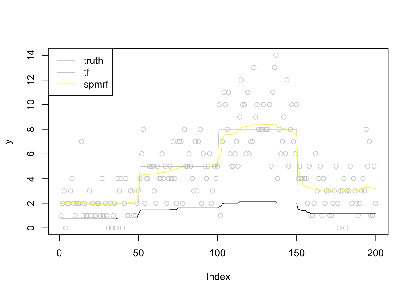

run time

paste0('tf run time:',round(t2_tf-t1_tf,2))

[1] "tf run time:0"

#paste0('tf_lasso run time:',round(t2_lasso-t1_lasso,2))
#paste0('susie run time:',round(t2_susie-t1_susie,2))
#paste0('btf run time:',round(t2_btf-t1_btf,2))
paste0('spmrf run time:',round(t2_spmrf-t1_spmrf,2))

[1] "spmrf run time:3.29"

sessionInfo()

R version 3.6.1 (2019-07-05)
Platform: x86_64-apple-darwin15.6.0 (64-bit)
Running under: macOS High Sierra 10.13.6

Matrix products: default
BLAS:   /Library/Frameworks/R.framework/Versions/3.6/Resources/lib/libRblas.0.dylib
LAPACK: /Library/Frameworks/R.framework/Versions/3.6/Resources/lib/libRlapack.dylib

locale:
[1] en_US.UTF-8/en_US.UTF-8/en_US.UTF-8/C/en_US.UTF-8/en_US.UTF-8

attached base packages:
[1] stats     graphics  grDevices utils     datasets  methods   base     

other attached packages:
 [1] rstan_2.19.2       ggplot2_3.2.1      StanHeaders_2.19.0
 [4] spmrf_1.2          btf_1.2            susieR_0.8.0      
 [7] glmnet_2.0-18      foreach_1.4.7      glmgen_0.0.3      
[10] genlasso_1.4       igraph_1.2.4.1     Matrix_1.2-17     
[13] MASS_7.3-51.4     

loaded via a namespace (and not attached):
 [1] tidyselect_0.2.5   xfun_0.10          purrr_0.3.2       
 [4] lattice_0.20-38    colorspace_1.4-1   htmltools_0.4.0   
 [7] stats4_3.6.1       loo_2.1.0          yaml_2.2.0        
[10] rlang_0.4.0        pkgbuild_1.0.5     later_1.0.0       
[13] pillar_1.4.2       glue_1.3.1         withr_2.1.2       
[16] matrixStats_0.55.0 stringr_1.4.0      munsell_0.5.0     
[19] gtable_0.3.0       workflowr_1.5.0    codetools_0.2-16  
[22] coda_0.19-3        evaluate_0.14      inline_0.3.15     
[25] knitr_1.25         callr_3.3.2        ps_1.3.0          
[28] httpuv_1.5.2       parallel_3.6.1     Rcpp_1.0.2        
[31] promises_1.1.0     backports_1.1.5    scales_1.0.0      
[34] fs_1.3.1           gridExtra_2.3      digest_0.6.21     
[37] stringi_1.4.3      processx_3.4.1     dplyr_0.8.3       
[40] grid_3.6.1         rprojroot_1.3-2    cli_1.1.0         
[43] tools_3.6.1        magrittr_1.5       lazyeval_0.2.2    
[46] tibble_2.1.3       crayon_1.3.4       whisker_0.4       
[49] pkgconfig_2.0.3    prettyunits_1.0.2  assertthat_0.2.1  
[52] rmarkdown_1.16     iterators_1.0.12   R6_2.4.0          
[55] git2r_0.26.1       compiler_3.6.1

Trend Filtering Examples

Dongyue Xie

2019-11-08

Introduction

Normal likelihood

Poisson likelihood