Smoothed Matrix Factorization using wavelet and EBMF
Dongyue Xie
Last updated: 2019-07-23
Checks: 7 0
Knit directory: FMF/
This reproducible R Markdown analysis was created with workflowr (version 1.4.0). The Checks tab describes the reproducibility checks that were applied when the results were created. The Past versions tab lists the development history.
Great! Since the R Markdown file has been committed to the Git repository, you know the exact version of the code that produced these results.
Great job! The global environment was empty. Objects defined in the global environment can affect the analysis in your R Markdown file in unknown ways. For reproduciblity it’s best to always run the code in an empty environment.
The command set.seed(20190719) was run prior to running the code in the R Markdown file. Setting a seed ensures that any results that rely on randomness, e.g. subsampling or permutations, are reproducible.
Great job! Recording the operating system, R version, and package versions is critical for reproducibility.
Nice! There were no cached chunks for this analysis, so you can be confident that you successfully produced the results during this run.
Great job! Using relative paths to the files within your workflowr project makes it easier to run your code on other machines.
Great! You are using Git for version control. Tracking code development and connecting the code version to the results is critical for reproducibility. The version displayed above was the version of the Git repository at the time these results were generated.
Note that you need to be careful to ensure that all relevant files for the analysis have been committed to Git prior to generating the results (you can use wflow_publish or wflow_git_commit). workflowr only checks the R Markdown file, but you know if there are other scripts or data files that it depends on. Below is the status of the Git repository when the results were generated:
Untracked files:
    Untracked:  docs/figure/SmoothPMD.Rmd/

Unstaged changes:
    Modified:   analysis/fpca.Rmd
Note that any generated files, e.g. HTML, png, CSS, etc., are not included in this status report because it is ok for generated content to have uncommitted changes.
These are the previous versions of the R Markdown and HTML files. If you’ve configured a remote Git repository (see ?wflow_git_remote), click on the hyperlinks in the table below to view them.
| File | Version | Author | Date | Message |
|---|---|---|---|---|
| Rmd | 2e047e3 | Dongyue Xie | 2019-07-23 | wflow_publish(c(“analysis/SmoothMF.Rmd”, “analysis/SmoothPMD.Rmd”)) |
| html | 666296b | Dongyue Xie | 2019-07-23 | Build site. |
| Rmd | cf686eb | Dongyue Xie | 2019-07-23 | wflow_publish(“analysis/SmoothMF.Rmd”) |
Introduction
Consider a matrix factorization problem \[Y = LF+E,\]
where \(Y\) is a \(N\times p\) matrix, \(L\) is a \(N\times K\) matrix, \(F\) is a \(K\times p\) matrix and \(E\) is a \(N\times p\) matrix of residuals.
We assume each row of \(F\) is smooth or spatially-structured. Then each row of \(Y\) is from a smooth function/curve with added noises. Matrix \(L\) is assumed to be sparse.
The question is how to estimate \(L\) and \(F\).
This is very similar to functional principal component analysis, which considers finding weights and principal components of a collection of curves. A common approach is adding a roughness penalty of the weights to obtain smooth estimates.
Here, we consider using a specific basis to represent the smooth curves - wavelet. Let \(W\) be the discrete wavelet transformation(DWT) matrix. We perform wavelet decomnposition on both sides then \[YW=LFW+EW,\] or \[\tilde{Y} = L\tilde{F}+\tilde{E}.\]
Now each row of \(\tilde{F}\) is sparse. We can then apply any penalized matrix factorization algorithm to \(\tilde{Y}\) to obtain sparse estimates of \(L\) and \(\tilde{F}\). Applying inverse DWT gives \(\hat{F}\).
Simulation
In this simulation study, we choose EBMF framework and compare it with the wavelet approach.
library(wavethresh)
library(flashr)
# wavelet-based matrix factorization
#'@ y: observed matrix
#'@ k: number of factors
#'@ filter.number, family: wavelet type

WaveEBMF = function(y,k,filter.number = 1,family = 'DaubExPhase'){
  N=nrow(y)
  p=ncol(y)
  W = GenW(n=p,filter.number = filter.number,family = family)
  y_tilde = y%*%W
  f2 = flash(y_tilde,Kmax=k,var_type = 'constant',backfit = T,verbose=F)
  f2_fitted = flash_get_ldf(f2)
  f_hat = (W%*%f2_fitted$f)
  return(list(f=f_hat,l=f2_fitted$l))
}
A single factor example
Simulate \(N=200\) and \(p=256\) under single-factor model \[l_i\sim \pi_0\delta_0+(1-\pi_0)\sum_{m=1}^5\frac{1}{5}N(0,\sigma^2_m)\]
Step function factor
\(f\) is a step function.
rmse = function(x1,x2){sqrt(mean((x1-x2)^2))}
set.seed(12345)
N = 200
p = 256
pi0 = 0.3
f = c(rep(2,p/4), rep(5, p/4), rep(6, p/4), rep(2, p/4))
l = c()
for (i in 1:N) {
  r = rbinom(1,1,pi0)
  if(r==1){
    l[i]=0
  }else{
      l[i] = mean(c(rnorm(1,0,sqrt(0.25)),rnorm(1,0,sqrt(0.5)),rnorm(1,0,sqrt(1)),
                    rnorm(1,0,sqrt(2)),rnorm(1,0,sqrt(4))))
      }
}
y = l%*%t(f)+matrix(rnorm(N*p,0,1),ncol=p)

# apply flash directly
f1 = flash(y,Kmax=1,var_type = 'constant',backfit = T,verbose=F)
f1 = flash_get_ldf(f1)

# apply wavelet transform

# use Haar wavelet

f2 = WaveEBMF(y,k=1)

paste('RMSE of l flash estimate:',round(rmse(f1$l,l/norm(l,'2')),5))
[1] "RMSE of l flash estimate: 0.00208"paste('RMSE of l Waveflash estimate:',round(rmse(f2$l,l/norm(l,'2')),5))[1] "RMSE of l Waveflash estimate: 0.00209"plot(f2$l,l/norm(l,'2'),xlab='Estimate',ylab='True l')
lines(f2$l,f2$l)
| Version | Author | Date |
|---|---|---|
| 666296b | Dongyue Xie | 2019-07-23 |
plot(f1$f,col = 2,type='l',xlab='',ylab='',main='Estimate of factors')
lines(f/norm(f,'2'),col='grey80',type='p')
lines(f2$f,col=4)
legend('topright',c('true f','flash','Waveflash'),col=c('grey80',2,4),lty=c(1,1,1))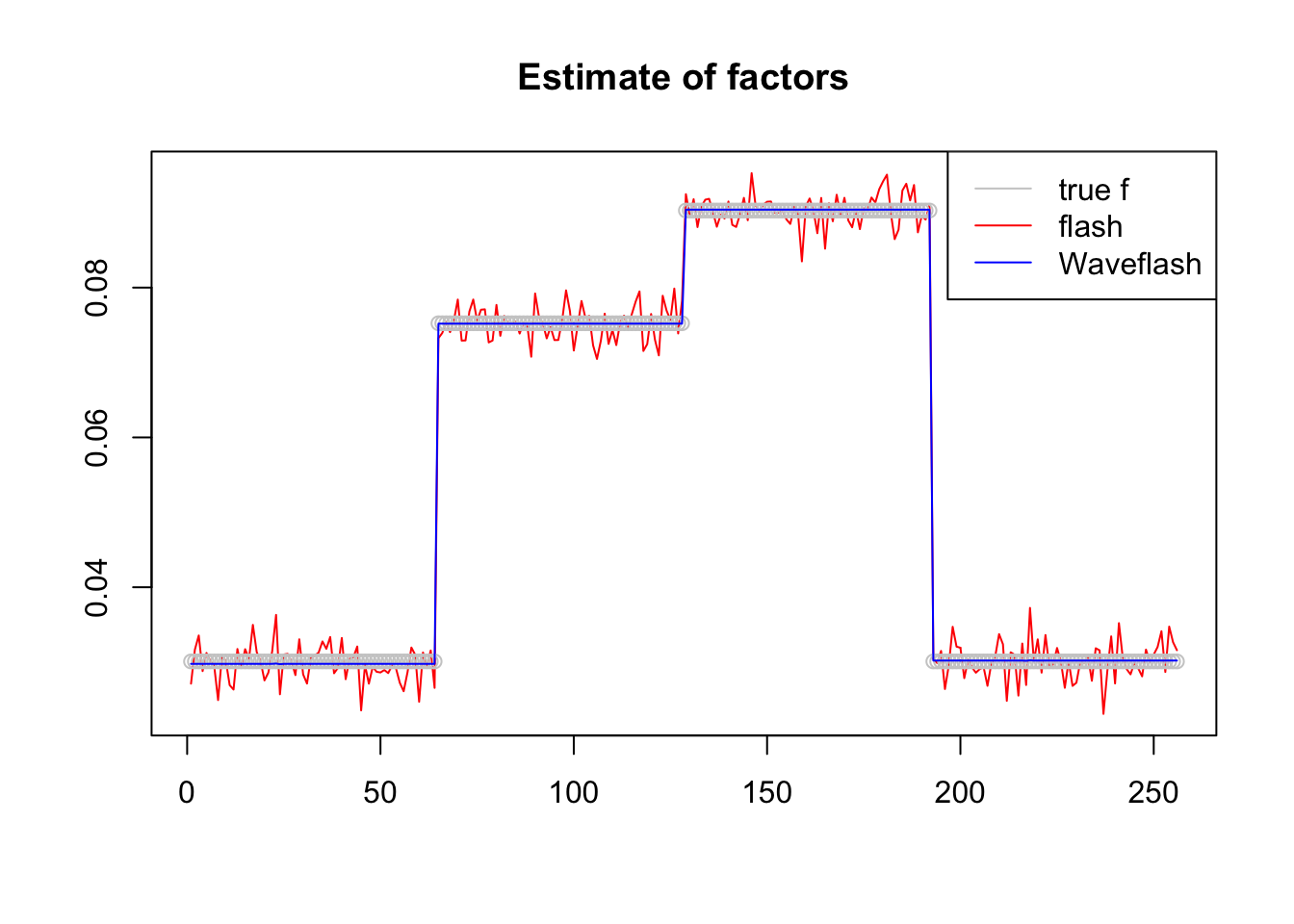
| Version | Author | Date |
|---|---|---|
| 666296b | Dongyue Xie | 2019-07-23 |
HeavySine function factor
f=DJ.EX(p,signal = 2)$heavi
y = l%*%t(f)+matrix(rnorm(N*p,0,1),ncol=p)

# apply flash directly
f1 = flash(y,Kmax=1,var_type = 'constant',backfit = F,verbose=F)
f1 = flash_get_ldf(f1)

# apply wavelet transform

# use symmlet10

f2 = WaveEBMF(y,k=1,filter.number = 10,family = 'DaubLeAsymm')

paste('RMSE of l flash estimate:',round(rmse(f1$l,l/norm(l,'2')),5))
[1] "RMSE of l flash estimate: 0.00428"paste('RMSE of l Waveflash estimate:',round(rmse(f2$l,l/norm(l,'2')),5))[1] "RMSE of l Waveflash estimate: 0.00421"plot(f2$l,l/norm(l,'2'),xlab='Estimate',ylab='True l')
lines(f2$l,f2$l)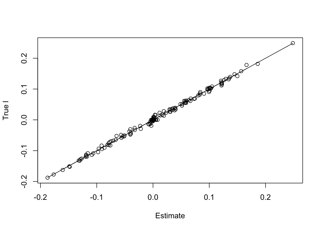
| Version | Author | Date |
|---|---|---|
| 666296b | Dongyue Xie | 2019-07-23 |
plot(f1$f,col = 2,type='l',xlab='',ylab='',main='Estimate of factors')
lines(f/norm(f,'2'),col='grey80',type='p')
lines(f2$f,col=4)
legend('topright',c('true f','flash','Waveflash'),col=c('grey80',2,4),lty=c(1,1,1))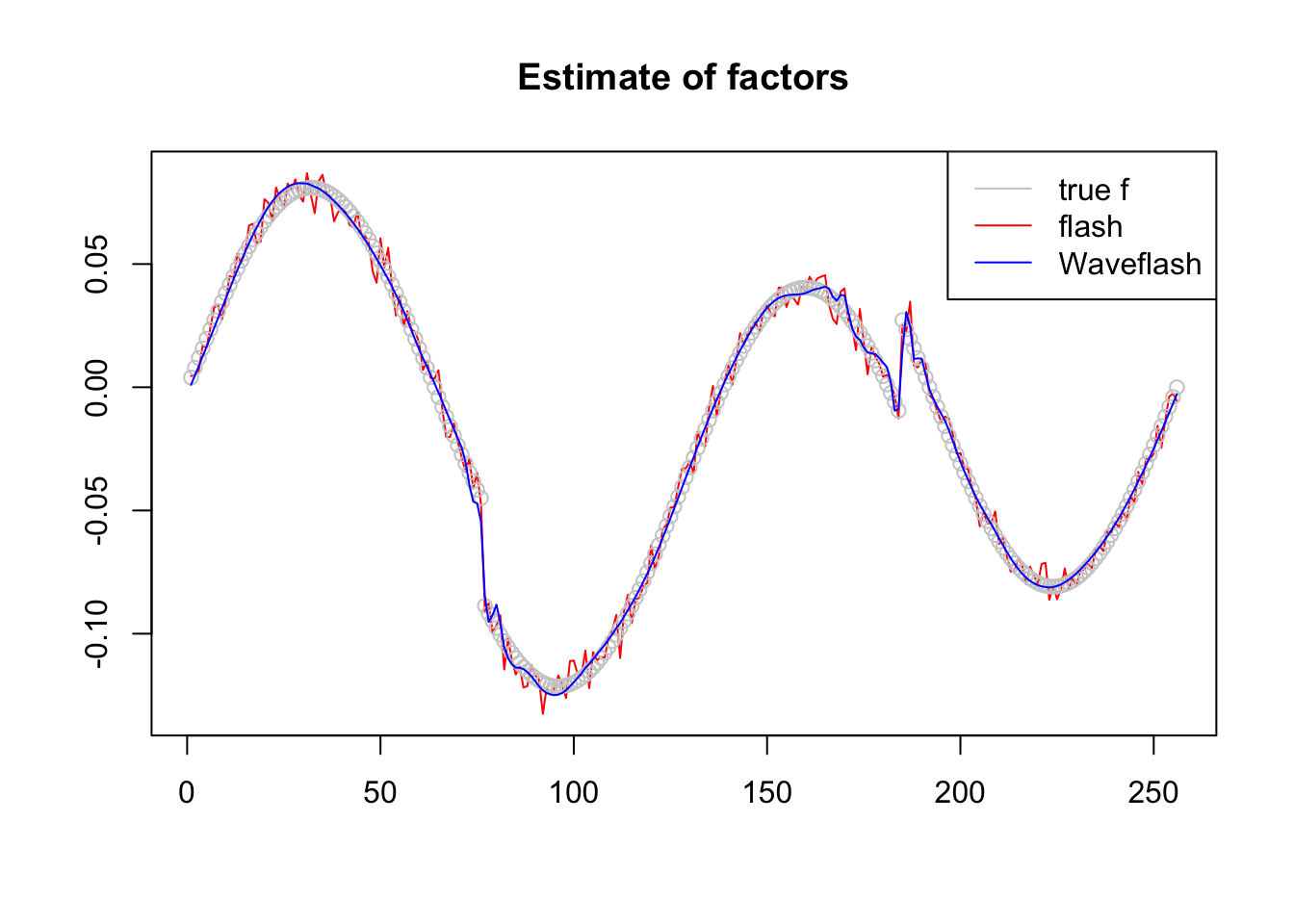
| Version | Author | Date |
|---|---|---|
| 666296b | Dongyue Xie | 2019-07-23 |
Spike function factor
spike.f = function(x) (0.75 * exp(-500 * (x - 0.23)^2) + 1.5 * exp(-2000 * (x - 0.33)^2) + 3 * exp(-8000 * (x - 0.47)^2) + 2.25 * exp(-16000 *
    (x - 0.69)^2) + 0.5 * exp(-32000 * (x - 0.83)^2))

t = 1:p/p
f = 2*spike.f(t)

y = l%*%t(f)+matrix(rnorm(N*p,0,1),ncol=p)

# apply flash directly
f1 = flash(y,Kmax=1,var_type = 'constant',backfit = F,verbose=F)
f1 = flash_get_ldf(f1)

# apply wavelet transform

# use symmlet10

f2 = WaveEBMF(y,k=1,filter.number = 10,family = 'DaubLeAsymm')

paste('RMSE of l flash estimate:',round(rmse(f1$l,l/norm(l,'2')),5))
[1] "RMSE of l flash estimate: 0.00897"paste('RMSE of l Waveflash estimate:',round(rmse(f2$l,l/norm(l,'2')),5))[1] "RMSE of l Waveflash estimate: 0.00905"plot(f2$l,l/norm(l,'2'),xlab='Estimate',ylab='True l')
lines(f2$l,f2$l)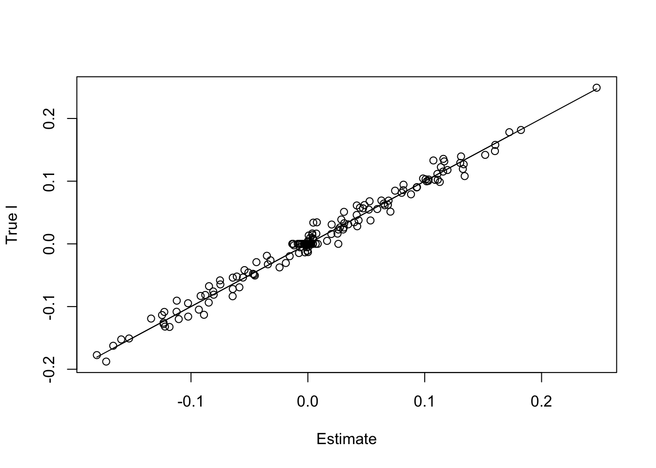
| Version | Author | Date |
|---|---|---|
| 666296b | Dongyue Xie | 2019-07-23 |
plot(f1$f,col = 2,type='l',xlab='',ylab='',main='Estimate of factors')
lines(f/norm(f,'2'),col='grey80',type='p')
lines(f2$f,col=4)
legend('topright',c('true f','flash','Waveflash'),col=c('grey80',2,4),lty=c(1,1,1))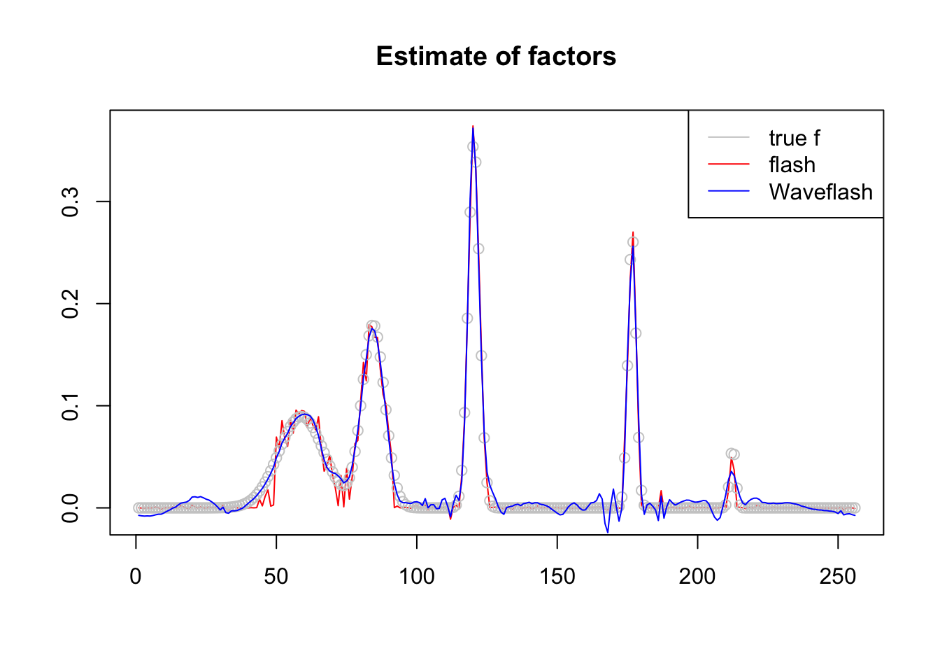
| Version | Author | Date |
|---|---|---|
| 666296b | Dongyue Xie | 2019-07-23 |
Three factors example
Simulate \(N=200\) and \(p=256\) under the factor model \[l_i\sim \pi_0\delta_0+(1-\pi_0)\sum_{m=1}^5\frac{1}{5}N(0,\sigma^2_m)\]
We set \(K=3\) and three factors are step function, Heavysine and spike functions.
K=3
set.seed(12345)
L = matrix(nrow=N,ncol=K)
for (i in 1:N) {
  for(j in 1:K){

    r = rbinom(1,1,pi0)
    if(r==1){
       L[i,j]=0
    }else{
      L[i,j] = mean(c(rnorm(1,0,sqrt(0.25)),rnorm(1,0,sqrt(0.5)),rnorm(1,0,sqrt(1)),
                    rnorm(1,0,sqrt(2)),rnorm(1,0,sqrt(4))))
    }
  }
}

f_1 = c(rep(2,p/4), rep(5, p/4), rep(6, p/4), rep(2, p/4))
f_2 = DJ.EX(p,signal = 2)$heavi
f_3 = 2*spike.f(t)
FF = rbind(f_1,f_2,f_3)
E = matrix(rnorm(N*p,0,1),ncol=p)
Y = L%*%FF + E

# apply flash directly
f1 = flash(Y,Kmax=3,var_type = 'constant',backfit = F,verbose=F)
f1 = flash_get_ldf(f1)

# apply wavelet transform

# use symmlet10

f2 = WaveEBMF(Y,k=3,filter.number = 10,family = 'DaubLeAsymm')


plot(-f1$f[,1],col = 2,type='l',xlab='',ylab='',main='Estimate of factor 1')
lines(f_1/norm(f_1,'2'),col='grey80',type='p')
lines(-f2$f[,1],col=4)
legend('topright',c('true f','flash','Waveflash'),col=c('grey80',2,4),lty=c(1,1,1))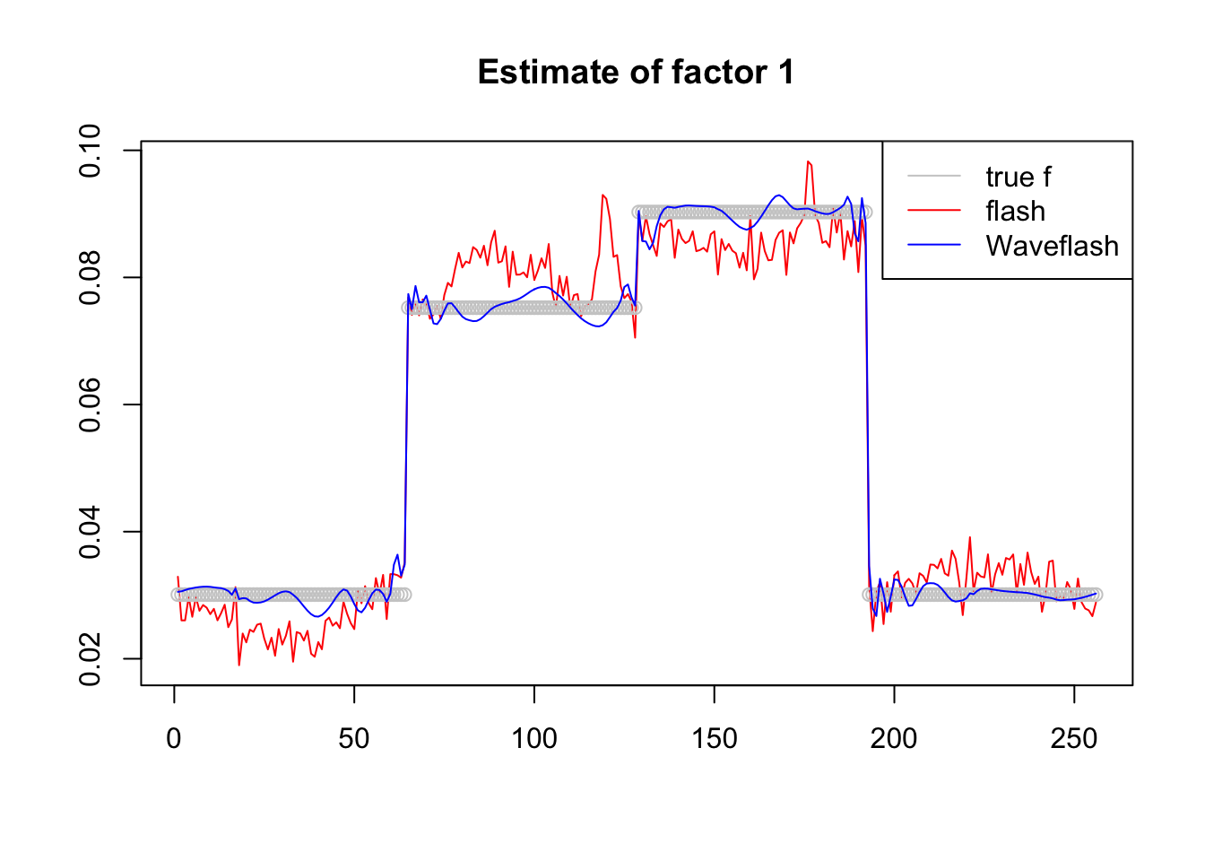
| Version | Author | Date |
|---|---|---|
| 666296b | Dongyue Xie | 2019-07-23 |
plot(-f1$f[,2],col = 2,type='l',xlab='',ylab='',main='Estimate of factor 1')
lines(f_2/norm(f_2,'2'),col='grey80',type='p')
lines(-f2$f[,2],col=4)
legend('topright',c('true f','flash','Waveflash'),col=c('grey80',2,4),lty=c(1,1,1))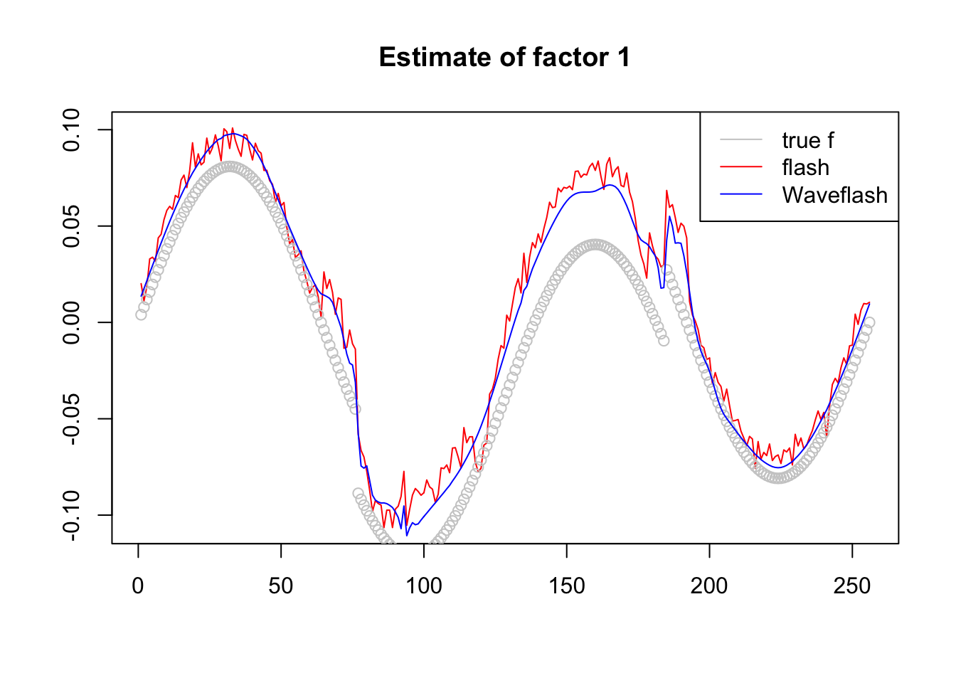
| Version | Author | Date |
|---|---|---|
| 666296b | Dongyue Xie | 2019-07-23 |
plot(f1$f[,3],col = 2,type='l',xlab='',ylab='',main='Estimate of factor 1')
lines(f_3/norm(f_3,'2'),col='grey80',type='p')
lines(f2$f[,3],col=4)
legend('topright',c('true f','flash','Waveflash'),col=c('grey80',2,4),lty=c(1,1,1))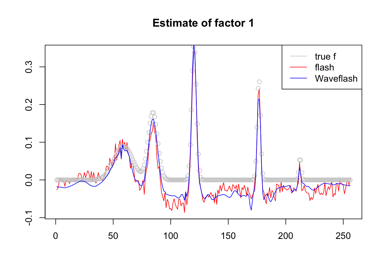
| Version | Author | Date |
|---|---|---|
| 666296b | Dongyue Xie | 2019-07-23 |
How about use Haar wavelet?
f2 = WaveEBMF(Y,k=3,filter.number = 1,family = 'DaubExPhase')


plot(-f1$f[,1],col = 2,type='l',xlab='',ylab='',main='Estimate of factor 1')
lines(f_1/norm(f_1,'2'),col='grey80',type='p')
lines(-f2$f[,1],col=4)
legend('topright',c('true f','flash','Waveflash'),col=c('grey80',2,4),lty=c(1,1,1))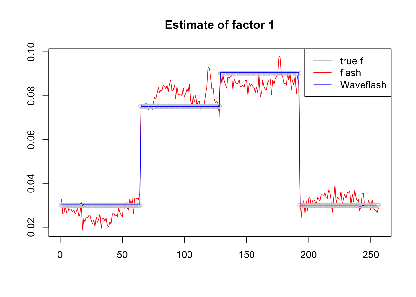
| Version | Author | Date |
|---|---|---|
| 666296b | Dongyue Xie | 2019-07-23 |
plot(-f1$f[,2],col = 2,type='l',xlab='',ylab='',main='Estimate of factor 1')
lines(f_2/norm(f_2,'2'),col='grey80',type='p')
lines(-f2$f[,2],col=4)
legend('topright',c('true f','flash','Waveflash'),col=c('grey80',2,4),lty=c(1,1,1))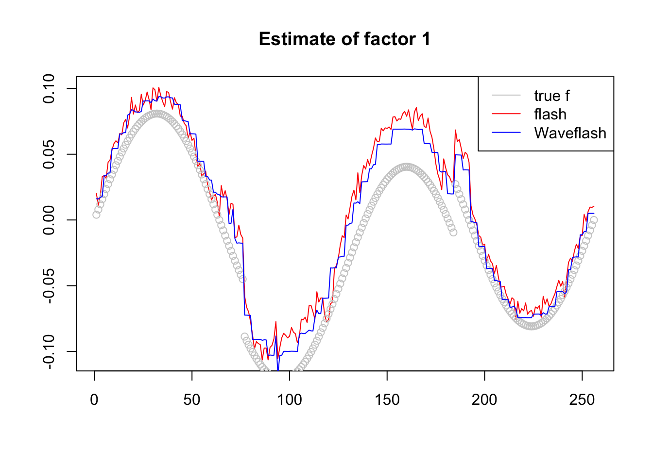
| Version | Author | Date |
|---|---|---|
| 666296b | Dongyue Xie | 2019-07-23 |
plot(f1$f[,3],col = 2,type='l',xlab='',ylab='',main='Estimate of factor 1')
lines(f_3/norm(f_3,'2'),col='grey80',type='p')
lines(f2$f[,3],col=4)
legend('topright',c('true f','flash','Waveflash'),col=c('grey80',2,4),lty=c(1,1,1))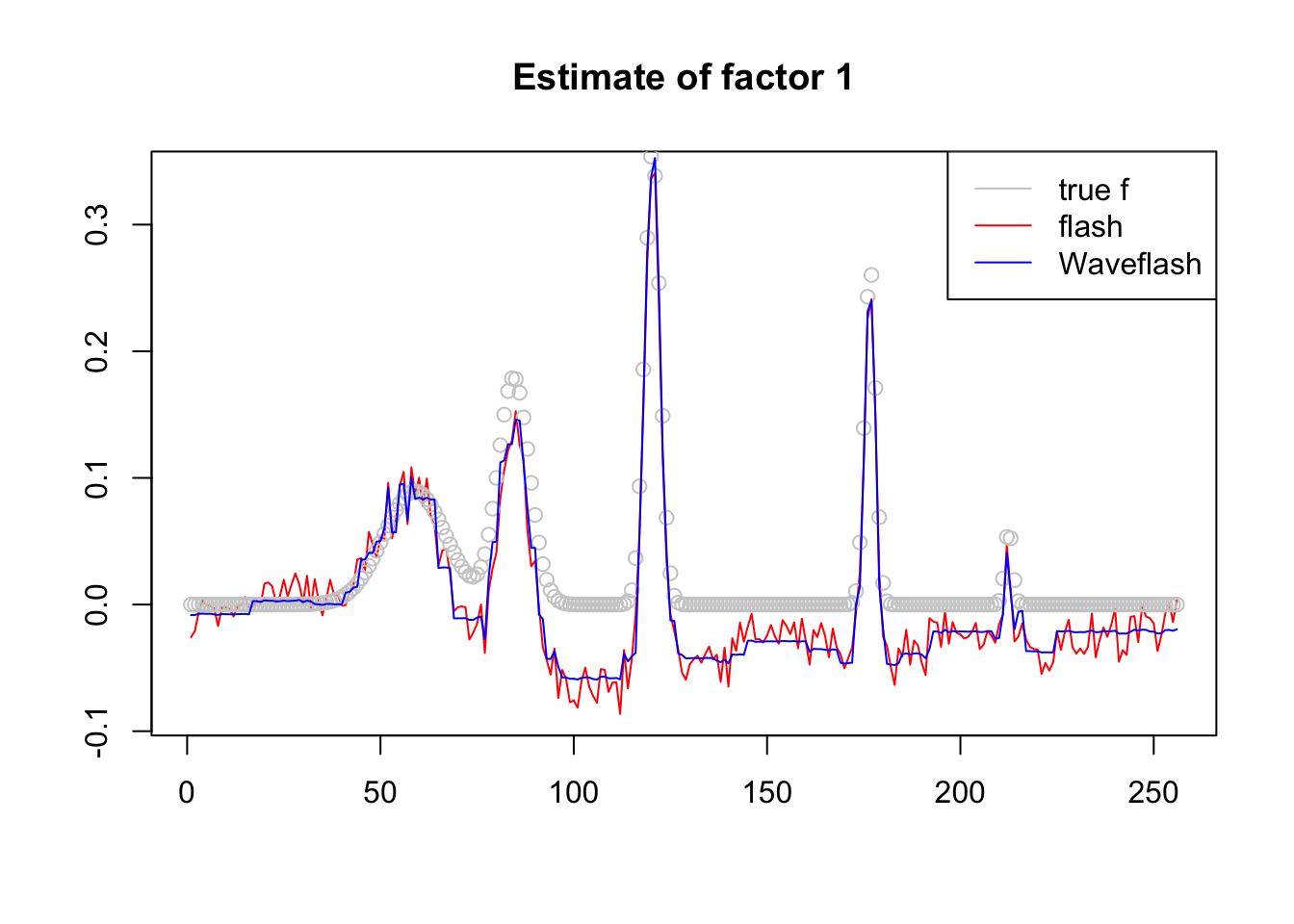
| Version | Author | Date |
|---|---|---|
| 666296b | Dongyue Xie | 2019-07-23 |
How about change the order of three factors?
FF = rbind(f_3,f_2,f_1)
Y = L%*%FF + E

# apply flash directly
f1 = flash(Y,Kmax=3,var_type = 'constant',backfit = F,verbose=F)
f1 = flash_get_ldf(f1)
f2 = WaveEBMF(Y,k=3,filter.number = 1,family = 'DaubExPhase')


plot(f1$f[,1],col = 2,type='l',xlab='',ylab='',main='Estimate of factor 1')
lines(f_1/norm(f_1,'2'),col='grey80',type='p')
lines(f2$f[,1],col=4)
legend('topright',c('true f','flash','Waveflash'),col=c('grey80',2,4),lty=c(1,1,1))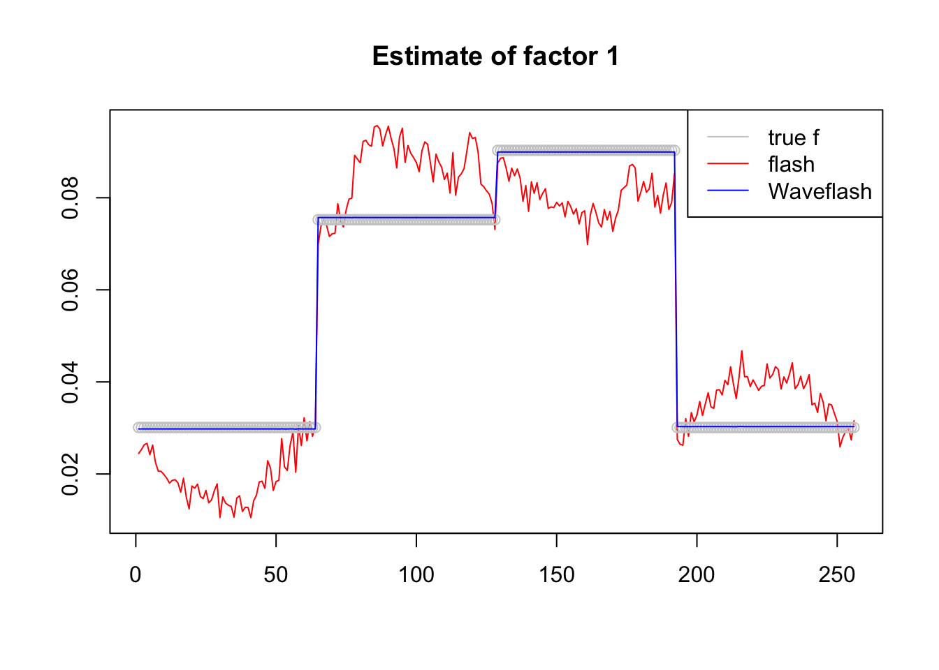
| Version | Author | Date |
|---|---|---|
| 666296b | Dongyue Xie | 2019-07-23 |
plot(-f1$f[,2],col = 2,type='l',xlab='',ylab='',main='Estimate of factor 1')
lines(f_2/norm(f_2,'2'),col='grey80',type='p')
lines(-f2$f[,2],col=4)
legend('topright',c('true f','flash','Waveflash'),col=c('grey80',2,4),lty=c(1,1,1))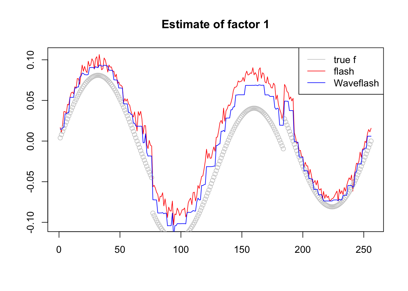
| Version | Author | Date |
|---|---|---|
| 666296b | Dongyue Xie | 2019-07-23 |
plot(-f1$f[,3],col = 2,type='l',xlab='',ylab='',main='Estimate of factor 1')
lines(f_3/norm(f_3,'2'),col='grey80',type='p')
lines(-f2$f[,3],col=4)
legend('topright',c('true f','flash','Waveflash'),col=c('grey80',2,4),lty=c(1,1,1))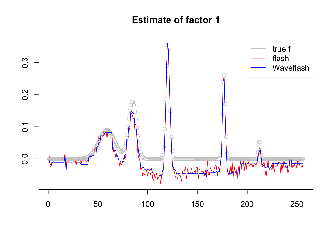
| Version | Author | Date |
|---|---|---|
| 666296b | Dongyue Xie | 2019-07-23 |
Try PMD
Summary
- The wavelet method gives smoother estimate of factors. The smoothness depends on the wavelet basis chosen.
- The signs of loadings and factors are not identifiable.
- Smash uses non-decimated DWT to give better estimate. If using NDWT in flash, there would be a lot more computational cost.
sessionInfo()R version 3.5.1 (2018-07-02)
Platform: x86_64-apple-darwin15.6.0 (64-bit)
Running under: macOS High Sierra 10.13.6
Matrix products: default
BLAS: /Library/Frameworks/R.framework/Versions/3.5/Resources/lib/libRblas.0.dylib
LAPACK: /Library/Frameworks/R.framework/Versions/3.5/Resources/lib/libRlapack.dylib
locale:
[1] en_US.UTF-8/en_US.UTF-8/en_US.UTF-8/C/en_US.UTF-8/en_US.UTF-8
attached base packages:
[1] stats graphics grDevices utils datasets methods base
other attached packages:
[1] flashr_0.6-6 wavethresh_4.6.8 MASS_7.3-51.1
loaded via a namespace (and not attached):
[1] Rcpp_1.0.1 plyr_1.8.4 bindr_0.1.1
[4] pillar_1.4.2 compiler_3.5.1 git2r_0.23.0
[7] workflowr_1.4.0 iterators_1.0.10 tools_3.5.1
[10] digest_0.6.20 evaluate_0.11 tibble_2.1.3
[13] gtable_0.3.0 lattice_0.20-35 pkgconfig_2.0.2
[16] rlang_0.4.0 Matrix_1.2-14 foreach_1.4.4
[19] yaml_2.2.0 parallel_3.5.1 ebnm_0.1-24
[22] bindrcpp_0.2.2 dplyr_0.7.8 stringr_1.3.1
[25] knitr_1.20 fs_1.2.6 tidyselect_0.2.5
[28] rprojroot_1.3-2 grid_3.5.1 glue_1.3.1
[31] R6_2.2.2 rmarkdown_1.10 mixsqp_0.1-97
[34] reshape2_1.4.3 purrr_0.2.5 ggplot2_3.2.0
[37] ashr_2.2-38 magrittr_1.5 whisker_0.3-2
[40] backports_1.1.4 scales_1.0.0 codetools_0.2-15
[43] htmltools_0.3.6 assertthat_0.2.1 softImpute_1.4
[46] colorspace_1.3-2 stringi_1.2.4 lazyeval_0.2.2
[49] doParallel_1.0.14 pscl_1.5.2 munsell_0.5.0
[52] truncnorm_1.0-8 SQUAREM_2017.10-1 crayon_1.3.4