poisson mean via penalized form

workflowr

• Summary
• Checks
• Past versions

Last updated: 2022-09-26

Checks: 7 0

Knit directory: gsmash/

This reproducible R Markdown analysis was created with workflowr (version 1.7.0). The Checks tab describes the reproducibility checks that were applied when the results were created. The Past versions tab lists the development history.

---

R Markdown file: up-to-date

Great! Since the R Markdown file has been committed to the Git repository, you know the exact version of the code that produced these results.

Environment: empty

Great job! The global environment was empty. Objects defined in the global environment can affect the analysis in your R Markdown file in unknown ways. For reproduciblity it’s best to always run the code in an empty environment.

Seed: set.seed(20220606)

The command set.seed(20220606) was run prior to running the code in the R Markdown file. Setting a seed ensures that any results that rely on randomness, e.g. subsampling or permutations, are reproducible.

Session information: recorded

Great job! Recording the operating system, R version, and package versions is critical for reproducibility.

Cache: none

Nice! There were no cached chunks for this analysis, so you can be confident that you successfully produced the results during this run.

File paths: relative

Great job! Using relative paths to the files within your workflowr project makes it easier to run your code on other machines.

Repository version: afbcd7b

Great! You are using Git for version control. Tracking code development and connecting the code version to the results is critical for reproducibility.

The results in this page were generated with repository version afbcd7b. See the Past versions tab to see a history of the changes made to the R Markdown and HTML files.

Note that you need to be careful to ensure that all relevant files for the analysis have been committed to Git prior to generating the results (you can use wflow_publish or wflow_git_commit). workflowr only checks the R Markdown file, but you know if there are other scripts or data files that it depends on. Below is the status of the Git repository when the results were generated:

Ignored files:
    Ignored:    .Rhistory
    Ignored:    .Rproj.user/

Untracked files:
    Untracked:  analysis/neg_binom_mean_lower_bound.Rmd
    Untracked:  analysis/neg_binom_mean_polya_gamma.Rmd
    Untracked:  code/poisson_mean/neg_binom_mean_lower_bound.R
    Untracked:  code/poisson_mean/neg_binom_mean_polya_gamma.R
    Untracked:  code/poisson_mean/pois_mean_GG.R
    Untracked:  code/poisson_mean/pois_mean_GG_opt.R
    Untracked:  code/poisson_mean/pois_mean_GMG.R
    Untracked:  code/poisson_mean/pois_mean_GMGM.R
    Untracked:  code/poisson_mean/test_example.R
    Untracked:  code/poisson_smooth/

Unstaged changes:
    Modified:   code/poisson_mean/pois_mean_penalized.R

Note that any generated files, e.g. HTML, png, CSS, etc., are not included in this status report because it is ok for generated content to have uncommitted changes.

---

These are the previous versions of the repository in which changes were made to the R Markdown (analysis/pois_mean_penalized.Rmd) and HTML (docs/pois_mean_penalized.html) files. If you’ve configured a remote Git repository (see ?wflow_git_remote), click on the hyperlinks in the table below to view the files as they were in that past version.

File	Version	Author	Date	Message
Rmd	afbcd7b	Dongyue Xie	2022-09-26	wflow_publish("analysis/pois_mean_penalized.Rmd")
html	3e8e7d2	Dongyue Xie	2022-09-26	Build site.
Rmd	f15734b	Dongyue Xie	2022-09-26	wflow_publish("analysis/pois_mean_penalized.Rmd")

---

Introduction

source("code/poisson_mean/pois_mean_penalized.R")

We solve the following Poisson mean problem by optimization method, \[x_i\sim Poisson(\exp\mu_i),\mu_i\sim g(\cdot)\]

We first generate data and fit poisson ash with log link.

library(ashr)
set.seed(12345)
w = c(0.8,0.2)
n = 100
mu = c(rnorm(n*w[1],0,0.01),rnorm(n*w[2],0,2))
x = rpois(n,exp(mu))

fit.ash = ash(x,1,lik=lik_pois(x,link='log'),mode=0)
fit.ash$fitted_g

$pi
 [1] 0.63235722 0.00000000 0.00000000 0.00000000 0.00000000 0.00000000
 [7] 0.00000000 0.00000000 0.00000000 0.00000000 0.00000000 0.00000000
[13] 0.00000000 0.12675581 0.13923979 0.00000000 0.02269363 0.00000000
[19] 0.00000000 0.00000000 0.02662634 0.00000000 0.00000000 0.05232721
[25] 0.00000000

$a
 [1]    0.00000000   -0.08044647   -0.11376848   -0.16089293   -0.22753697
 [6]   -0.32178586   -0.45507393   -0.64357173   -0.91014787   -1.28714346
[11]   -1.82029573   -2.57428692   -3.64059147   -5.14857383   -7.28118294
[16]  -10.29714766  -14.56236588  -20.59429533  -29.12473176  -41.18859065
[21]  -58.24946352  -82.37718131 -116.49892703 -164.75436261 -232.99785407

$b
 [1]   0.00000000   0.08044647   0.11376848   0.16089293   0.22753697
 [6]   0.32178586   0.45507393   0.64357173   0.91014787   1.28714346
[11]   1.82029573   2.57428692   3.64059147   5.14857383   7.28118294
[16]  10.29714766  14.56236588  20.59429533  29.12473176  41.18859065
[21]  58.24946352  82.37718131 116.49892703 164.75436261 232.99785407

attr(,"class")
[1] "unimix"
attr(,"row.names")
 [1]  1  2  3  4  5  6  7  8  9 10 11 12 13 14 15 16 17 18 19 20 21 22 23 24 25

plot(x,col='grey50',main='ash fit',ylim=c(0,150))
lines(fit.ash$result$PosteriorMean,col=4)
legend('topleft',c('data','ash posterior mean'), pch=c(1,NA),lty=c(NA,1),col=c('grey50',4))

plot(mu,col='grey50',main='ash fit',ylim=c(-2,6))
lines(log(fit.ash$result$PosteriorMean))
legend('topleft',c('true mu','log(ash posterior mean)'), pch=c(1,NA),lty=c(NA,1),col=c('grey50',4))

known prior

Now we fit the penalize poisson mean problem with known prior.

Use Nelder-Mead:

grid=c(0.01,2)
fit = pois_mean_penalized_optim(x,w=w,grid=grid,est_w=FALSE,z_init = log(1+x),opt_method = 'Nelder-Mead')
plot(L_grad_known_g(fit$fit$par,x,w,grid),ylab='gradient',main='check gradient')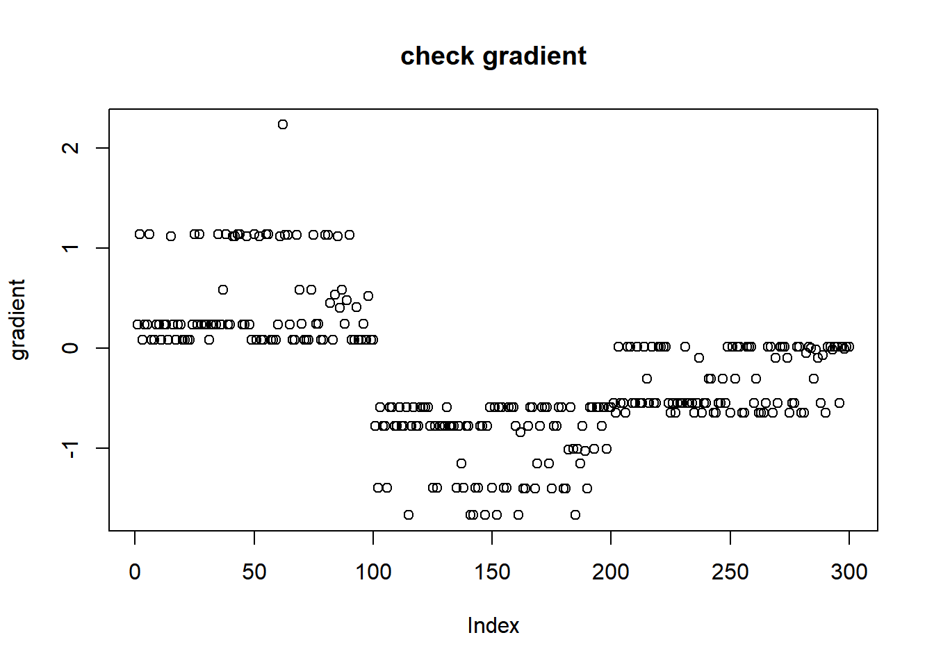

plot(fit$z,col='grey50')
lines(log(1+x),type='p',pch=8,col='grey50')
lines(mu,col='grey80',type='p',pch=20)
lines(fit$m,col=4)
legend('topleft',c('log(1+x)','z','true mu','mu hat'), pch=c(8,1,20,NA),lty=c(NA,NA,NA,1),col=c('grey50','grey50','grey80',4))

fit$s2

  [1] 0.503943270 0.335962180 1.007886541 0.503943270 0.503943270 0.335962180
  [7] 1.007886541 1.007886541 0.503943270 0.503943270 1.007886541 0.503943270
 [13] 0.503943270 1.007886541 0.251971635 0.503943270 1.007886541 0.503943270
 [19] 0.503943270 1.007886541 1.007886541 1.007886541 1.007886541 0.503943270
 [25] 0.335962180 0.503943270 0.335962180 0.503943270 0.503943270 0.503943270
 [31] 1.007886541 0.503943270 0.503943270 0.503943270 0.335962180 0.503943270
 [37] 0.201577308 0.335962180 0.503943270 0.503943270 0.251971635 0.251971635
 [43] 0.335962180 0.335962180 0.503943270 0.503943270 0.251971635 0.503943270
 [49] 1.007886541 0.335962180 1.007886541 0.251971635 1.007886541 1.007886541
 [55] 0.335962180 0.335962180 1.007886541 1.007886541 1.007886541 0.503943270
 [61] 0.251971635 0.335962180 0.335962180 0.335962180 0.503943270 1.007886541
 [67] 1.007886541 0.335962180 0.201577308 0.503943270 1.007886541 1.007886541
 [73] 1.007886541 0.201577308 0.335962180 0.503943270 0.503943270 1.007886541
 [79] 1.007886541 0.335962180 0.335962180 0.091626049 1.007886541 0.008541411
 [85] 0.251971635 0.020997636 0.201577308 0.503943270 0.167981090 0.335962180
 [91] 1.007886541 1.007886541 0.025197164 1.007886541 1.007886541 0.503943270
 [97] 1.007886541 0.012598582 1.007886541 1.007886541

L_known_g(fit$fit$par,x,w,grid)

[1] -688.6274

Use BFGS:

fit = pois_mean_penalized_optim(x,w=w,grid=grid,est_w=FALSE,z_init = log(1+x),opt_method = 'BFGS')
plot(L_grad_known_g(fit$fit$par,x,w,grid),ylab='gradient',main='check gradient')

plot(fit$z,col='grey50')
lines(log(1+x),type='p',pch=8,col='grey50')
lines(mu,col='grey80',type='p',pch=20)
lines(fit$m,col=4)
legend('topleft',c('log(1+x)','z','true mu','mu hat'), pch=c(8,1,20,NA),lty=c(NA,NA,NA,1),col=c('grey50','grey50','grey80',4))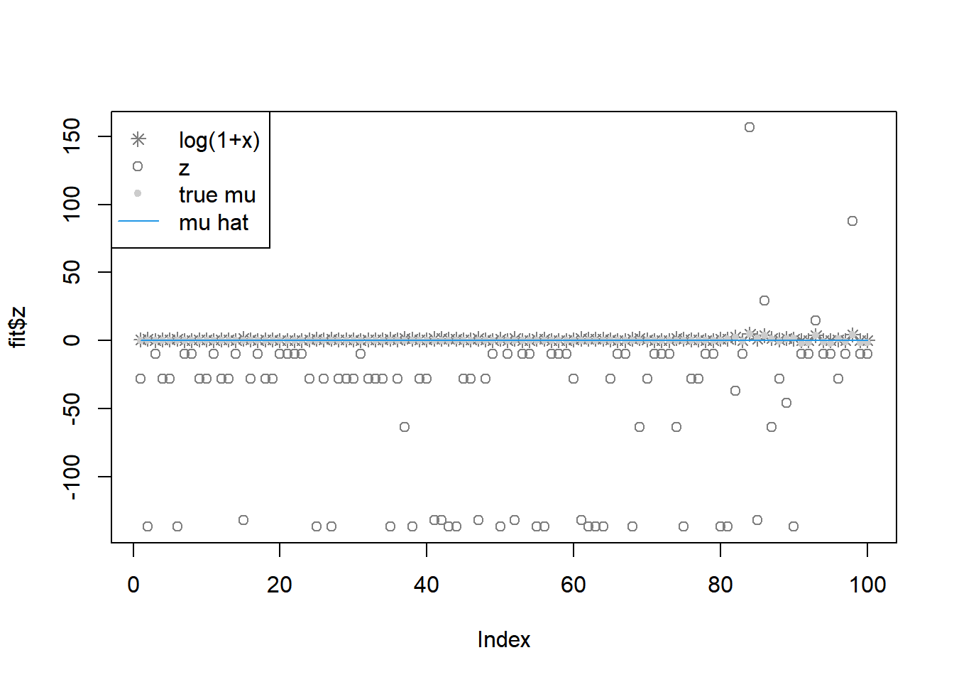

fit$s2

  [1] 1.563562e+42 3.787427e+75 4.879849e+30 1.563562e+42 1.563562e+42
  [6] 3.787427e+75 4.879849e+30 4.879849e+30 1.563562e+42 1.563562e+42
 [11] 4.879849e+30 1.563562e+42 1.563562e+42 4.879849e+30 8.588190e+86
 [16] 1.563562e+42 4.879849e+30 1.563562e+42 1.563562e+42 4.879849e+30
 [21] 4.879849e+30 4.879849e+30 4.879849e+30 1.563562e+42 3.787427e+75
 [26] 1.563562e+42 3.787427e+75 1.563562e+42 1.563562e+42 1.563562e+42
 [31] 4.879849e+30 1.563562e+42 1.563562e+42 1.563562e+42 3.787427e+75
 [36] 1.563562e+42 1.008232e+59 3.787427e+75 1.563562e+42 1.563562e+42
 [41] 8.588190e+86 8.588190e+86 3.787427e+75 3.787427e+75 1.563562e+42
 [46] 1.563562e+42 8.588190e+86 1.563562e+42 4.879849e+30 3.787427e+75
 [51] 4.879849e+30 8.588190e+86 4.879849e+30 4.879849e+30 3.787427e+75
 [56] 3.787427e+75 4.879849e+30 4.879849e+30 4.879849e+30 1.563562e+42
 [61] 8.588190e+86 3.787427e+75 3.787427e+75 3.787427e+75 1.563562e+42
 [66] 4.879849e+30 4.879849e+30 3.787427e+75 1.008232e+59 1.563562e+42
 [71] 4.879849e+30 4.879849e+30 4.879849e+30 1.008232e+59 3.787427e+75
 [76] 1.563562e+42 1.563562e+42 4.879849e+30 4.879849e+30 3.787427e+75
 [81] 3.787427e+75 6.174722e+50 4.879849e+30 5.189492e+48 8.588190e+86
 [86] 4.763309e+49 1.008232e+59 1.563562e+42 4.250852e+50 3.787427e+75
 [91] 4.879849e+30 4.879849e+30 7.775782e+49 4.879849e+30 4.879849e+30
 [96] 1.563562e+42 4.879849e+30 1.306805e+49 4.879849e+30 4.879849e+30

L_known_g(fit$fit$par,x,w,grid)

[1] -471183.7

Use CG:

fit = pois_mean_penalized_optim(x,w=w,grid=grid,est_w=FALSE,z_init = log(1+x),opt_method = 'CG')
plot(L_grad_known_g(fit$fit$par,x,w,grid),ylab='gradient',main='check gradient')

plot(fit$z,col='grey50')
lines(log(1+x),type='p',pch=8,col='grey50')
lines(mu,col='grey80',type='p',pch=20)
lines(fit$m,col=4)
legend('topleft',c('log(1+x)','z','true mu','mu hat'), pch=c(8,1,20,NA),lty=c(NA,NA,NA,1),col=c('grey50','grey50','grey80',4))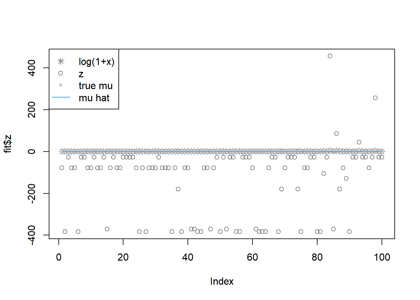

fit$s2

  [1] 1.335038e+125 4.357316e+214  5.025312e+85 1.335038e+125 1.335038e+125
  [6] 4.357316e+214  5.025312e+85  5.025312e+85 1.335038e+125 1.335038e+125
 [11]  5.025312e+85 1.335038e+125 1.335038e+125  5.025312e+85 2.279027e+245
 [16] 1.335038e+125  5.025312e+85 1.335038e+125 1.335038e+125  5.025312e+85
 [21]  5.025312e+85  5.025312e+85  5.025312e+85 1.335038e+125 4.357316e+214
 [26] 1.335038e+125 4.357316e+214 1.335038e+125 1.335038e+125 1.335038e+125
 [31]  5.025312e+85 1.335038e+125 1.335038e+125 1.335038e+125 4.357316e+214
 [36] 1.335038e+125 5.869611e+167 4.357316e+214 1.335038e+125 1.335038e+125
 [41] 2.279027e+245 2.279027e+245 4.357316e+214 4.357316e+214 1.335038e+125
 [46] 1.335038e+125 2.279027e+245 1.335038e+125  5.025312e+85 4.357316e+214
 [51]  5.025312e+85 2.279027e+245  5.025312e+85  5.025312e+85 4.357316e+214
 [56] 4.357316e+214  5.025312e+85  5.025312e+85  5.025312e+85 1.335038e+125
 [61] 2.279027e+245 4.357316e+214 4.357316e+214 4.357316e+214 1.335038e+125
 [66]  5.025312e+85  5.025312e+85 4.357316e+214 5.869611e+167 1.335038e+125
 [71]  5.025312e+85  5.025312e+85  5.025312e+85 5.869611e+167 4.357316e+214
 [76] 1.335038e+125 1.335038e+125  5.025312e+85  5.025312e+85 4.357316e+214
 [81] 4.357316e+214 1.036774e+144  5.025312e+85 1.571839e+125 2.279027e+245
 [86] 5.419367e+140 5.869611e+167 1.335038e+125 3.669941e+143 4.357316e+214
 [91]  5.025312e+85  5.025312e+85 5.736992e+141  5.025312e+85  5.025312e+85
 [96] 1.335038e+125  5.025312e+85 2.040635e+135  5.025312e+85  5.025312e+85

L_known_g(fit$fit$par,x,w,grid)

[1] -3254344

Use nleqslv for solving gradient = 0 directly.

library(nleqslv)
grid=c(0.01,2)
fit = pois_mean_penalized_nleqslv(x,w=w,grid=grid,est_w=FALSE,z_init = log(1+x),opt_method = 'Broyden')
plot(L_grad_known_g(fit$fit$x,x,w,grid),ylab='gradient',main='check gradient')

plot(fit$z,col='grey50')
lines(log(1+x),type='p',pch=8,col='grey50')
lines(mu,col='grey80',type='p',pch=20)
lines(fit$m,col=4)
legend('topleft',c('log(1+x)','z','true mu','mu hat'), pch=c(8,1,20,NA),lty=c(NA,NA,NA,1),col=c('grey50','grey50','grey80',4))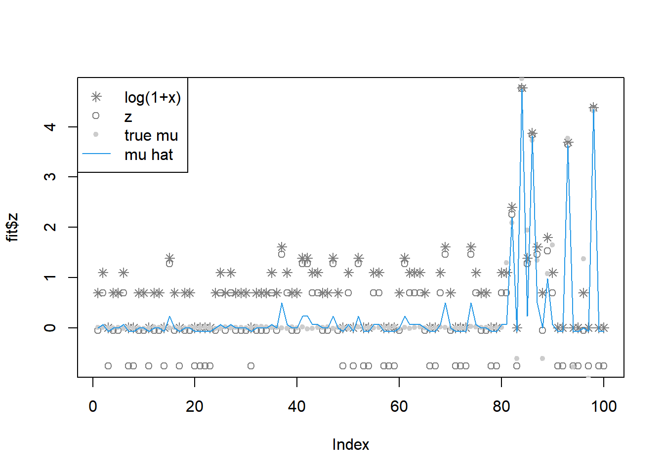

fit$s2

  [1] 1.008880159 0.879275042 1.152719331 1.008880159 1.008880159 0.879275042
  [7] 1.152719331 1.152719331 1.008880159 1.008880159 1.152719331 1.008880159
 [13] 1.008880159 1.152719331 0.667709938 1.008880159 1.152719331 1.008880159
 [19] 1.008880159 1.152719331 1.152719331 1.152719331 1.152719331 1.008880159
 [25] 0.879275042 1.008880159 0.879275042 1.008880159 1.008880159 1.008880159
 [31] 1.152719331 1.008880159 1.008880159 1.008880159 0.879275042 1.008880159
 [37] 0.474556224 0.879275042 1.008880159 1.008880159 0.667709938 0.667709938
 [43] 0.879275042 0.879275042 1.008880159 1.008880159 0.667709938 1.008880159
 [49] 1.152719331 0.879275042 1.152719331 0.667709938 1.152719331 1.152719331
 [55] 0.879275042 0.879275042 1.152719331 1.152719331 1.152719331 1.008880159
 [61] 0.667709938 0.879275042 0.879275042 0.879275042 1.008880159 1.152719331
 [67] 1.152719331 0.879275042 0.474556224 1.008880159 1.152719331 1.152719331
 [73] 1.152719331 0.474556224 0.879275042 1.008880159 1.008880159 1.152719331
 [79] 1.152719331 0.879275042 0.879275042 0.111429385 1.152719331 0.008671599
 [85] 0.667709938 0.021951297 0.474556224 1.008880159 0.307423274 0.879275042
 [91] 1.152719331 1.152719331 0.026592590 1.152719331 1.152719331 1.008880159
 [97] 1.152719331 0.012916529 1.152719331 1.152719331

L_known_g(fit$fit$x,x,w,grid)

[1] -733.7425

fit = pois_mean_penalized_nleqslv(x,w=w,grid=grid,est_w=FALSE,z_init = log(1+x),opt_method = 'Newton')
plot(L_grad_known_g(fit$fit$x,x,w,grid),ylab='gradient',main='check gradient')

plot(fit$z,col='grey50')
lines(log(1+x),type='p',pch=8,col='grey50')
lines(mu,col='grey80',type='p',pch=20)
lines(fit$m,col=4)
legend('topleft',c('log(1+x)','z','true mu','mu hat'), pch=c(8,1,20,NA),lty=c(NA,NA,NA,1),col=c('grey50','grey50','grey80',4))

fit$s2

  [1]  1.005338369  0.872197937  1.151864543  1.005338369  1.005338369
  [6]  0.872197937  1.151864543  1.151864543  1.005338369  1.005338369
 [11]  1.151864543  1.005338369  1.005338369  1.151864543 38.218242360
 [16]  1.005338369  1.151864543  1.005338369  1.005338369  1.151864543
 [21]  1.151864543  1.151864543  1.151864543  1.005338369  0.872197937
 [26]  1.005338369  0.872197937  1.005338369  1.005338369  1.005338369
 [31]  1.151864543  1.005338369  1.005338369  1.005338369  0.872197937
 [36]  1.005338369  0.475474444  0.872197937  1.005338369  1.005338369
 [41] 38.218242360 38.218242360  0.872197937  0.872197937  1.005338369
 [46]  1.005338369 38.218242360  1.005338369  1.151864543  0.872197937
 [51]  1.151864543 38.218242360  1.151864543  1.151864543  0.872197937
 [56]  0.872197937  1.151864543  1.151864543  1.151864543  1.005338369
 [61] 38.218242360  0.872197937  0.872197937  0.872197937  1.005338369
 [66]  1.151864543  1.151864543  0.872197937  0.475474444  1.005338369
 [71]  1.151864543  1.151864543  1.151864543  0.475474444  0.872197937
 [76]  1.005338369  1.005338369  1.151864543  1.151864543  0.872197937
 [81]  0.872197937  0.111334228  1.151864543  0.008670817 38.218242360
 [86]  0.021946771  0.475474444  1.005338369  0.306481214  0.872197937
 [91]  1.151864543  1.151864543  0.026586098  1.151864543  1.151864543
 [96]  1.005338369  1.151864543  0.012914866  1.151864543  1.151864543

L_known_g(fit$fit$x,x,w,grid)

[1] -645.5743

estimating prior

fit.ash = ashr::ash(log(x+0.01),sqrt(exp(-log(x+0.01))),pointmass=F,mixcompdist='normal',prior='uniform')
grid = fit.ash$fitted_g$sd
K = length(grid)

opt_method = ‘BFGS’

fit = pois_mean_penalized_optim(x,w=NULL,grid=grid,est_w=TRUE,z_init = log(1+x),opt_method = 'BFGS')

round(fit$w,3)

 [1] 0.000 0.000 0.000 0.000 0.000 0.000 0.000 0.000 0.000 0.000 0.000 0.001
[13] 0.997 0.002 0.000 0.000 0.000 0.000 0.000 0.000 0.000 0.000

plot(grid,fit$w)

plot(L_grad(fit$fit$par,x,grid),ylab='gradient',main='check gradient')

plot(fit$z,col='grey50')
lines(log(1+x),type='p',pch=8,col='grey50')
lines(mu,col='grey80',type='p',pch=20)
lines(fit$m,col=4)
legend('topleft',c('log(1+x)','z','true mu','mu hat'), pch=c(8,1,20,NA),lty=c(NA,NA,NA,1),col=c('grey50','grey50','grey80',4))

fit$s2

  [1] 1.662263e+289 2.651347e+214  1.701144e+72 1.661045e+289 1.662265e+289
  [6] 3.621524e+213  1.701144e+72  1.701144e+72 1.662227e+289 1.662234e+289
 [11]  1.701144e+72 1.662234e+289 1.661032e+289  1.701144e+72 1.902646e+232
 [16] 1.662234e+289  1.701144e+72 1.661032e+289 1.662226e+289  1.701144e+72
 [21]  1.701144e+72  1.701144e+72  1.701144e+72 1.660996e+289 3.256023e+214
 [26] 1.662257e+289 3.254388e+214 1.662226e+289 1.662227e+289 1.662220e+289
 [31]  1.701144e+72 1.662233e+289 1.662253e+289 1.662233e+289 2.653101e+214
 [36] 1.662262e+289 5.357096e+238 2.568121e+214 1.662230e+289 1.661932e+289
 [41] 1.902646e+232 1.902646e+232 4.773782e+278 4.773723e+278 1.662243e+289
 [46] 1.662246e+289 1.902646e+232 1.662219e+289  1.701144e+72 9.934917e+209
 [51]  1.701144e+72 1.902646e+232  1.701144e+72  1.701144e+72 4.773723e+278
 [56] 4.773723e+278  1.701144e+72  1.701144e+72  1.701144e+72 1.662265e+289
 [61] 1.902646e+232 1.892733e+215 1.454471e+188 1.890177e+215 1.661031e+289
 [66]  1.701144e+72  1.701144e+72 7.501820e+214 5.357096e+238 1.661040e+289
 [71]  1.701144e+72  1.701144e+72  1.701144e+72 5.357096e+238 7.037162e+241
 [76] 1.662257e+289 1.661040e+289  1.701144e+72  1.701144e+72 3.413647e+214
 [81] 1.465413e+214 2.261519e+123  1.701144e+72  3.589303e+78 1.902646e+232
 [86]  1.017289e+84 5.357096e+238 1.662260e+289 4.568985e+216 2.567518e+214
 [91]  1.701144e+72  1.701144e+72  5.844931e+85  1.701144e+72  1.701144e+72
 [96] 1.662256e+289  1.701144e+72  7.675118e+53  1.701144e+72  1.701144e+72

opt_method = ‘Nelder-Mead’

fit = pois_mean_penalized_optim(x,w=NULL,grid=grid,est_w=TRUE,z_init = log(1+x),opt_method = 'Nelder-Mead')

round(fit$w,3)

 [1] 0.047 0.047 0.047 0.047 0.047 0.047 0.047 0.047 0.047 0.047 0.047 0.047
[13] 0.047 0.047 0.047 0.047 0.047 0.047 0.047 0.047 0.047 0.018

plot(grid,fit$w)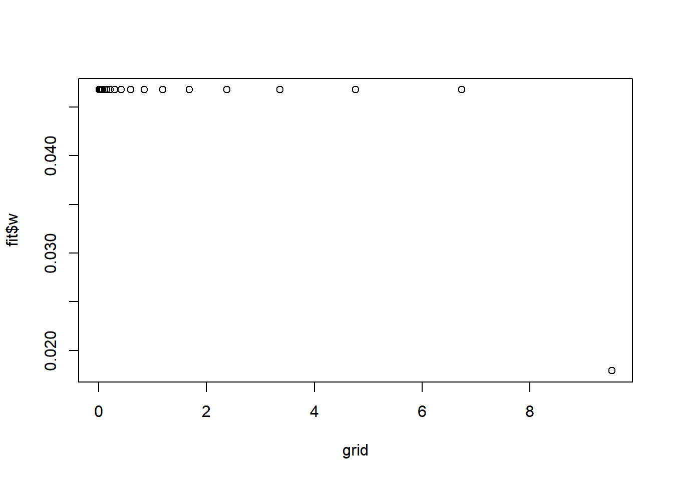

plot(L_grad(fit$fit$par,x,grid),ylab='gradient',main='check gradient')

plot(fit$z,col='grey50')
lines(log(1+x),type='p',pch=8,col='grey50')
lines(mu,col='grey80',type='p',pch=20)
lines(fit$m,col=4)
legend('topleft',c('log(1+x)','z','true mu','mu hat'), pch=c(8,1,20,NA),lty=c(NA,NA,NA,1),col=c('grey50','grey50','grey80',4))

fit$s2

  [1] 0.50226581 0.33484387 1.00453162 0.50226581 0.50226581 0.33484387
  [7] 1.00453162 1.00453162 0.50226581 0.50226581 1.00453162 0.50226581
 [13] 0.50226581 1.00453162 0.25113290 0.50226581 1.00453162 0.50226581
 [19] 0.50226581 1.00453162 1.00453162 1.00453162 1.00453162 0.50226581
 [25] 0.33484387 0.50226581 0.33484387 0.50226581 0.50226581 0.50226581
 [31] 1.00453162 0.50226581 0.50226581 0.50226581 0.33484387 0.50226581
 [37] 0.20090632 0.33484387 0.50226581 0.50226581 0.25113290 0.25113290
 [43] 0.33484387 0.33484387 0.50226581 0.50226581 0.25113290 0.50226581
 [49] 1.00453162 0.33484387 1.00453162 0.25113290 1.00453162 1.00453162
 [55] 0.33484387 0.33484387 1.00453162 1.00453162 1.00453162 0.50226581
 [61] 0.25113290 0.33484387 0.33484387 0.33484387 0.50226581 1.00453162
 [67] 1.00453162 0.33484387 0.20090632 0.50226581 1.00453162 1.00453162
 [73] 1.00453162 0.20090632 0.33484387 0.50226581 0.50226581 1.00453162
 [79] 1.00453162 0.33484387 0.33484387 0.09132106 1.00453162 0.00851298
 [85] 0.25113290 0.02092774 0.20090632 0.50226581 0.16742194 0.33484387
 [91] 1.00453162 1.00453162 0.02511329 1.00453162 1.00453162 0.50226581
 [97] 1.00453162 0.01255665 1.00453162 1.00453162

opt_method = ‘L-BFGS-B’

fit = pois_mean_penalized_optim(x,w=NULL,grid=grid,est_w=TRUE,z_init = log(1+x),opt_method = 'L-BFGS-B')

round(fit$w,3)

 [1] 0.058 0.058 0.058 0.058 0.058 0.058 0.058 0.059 0.061 0.065 0.072 0.086
[13] 0.111 0.112 0.029 0.001 0.000 0.000 0.000 0.000 0.000 0.000

plot(grid,fit$w)

plot(L_grad(fit$fit$par,x,grid),ylab='gradient',main='check gradient')

plot(fit$z,col='grey50')
lines(log(1+x),type='p',pch=8,col='grey50')
lines(mu,col='grey80',type='p',pch=20)
lines(fit$m,col=4)
legend('topleft',c('log(1+x)','z','true mu','mu hat'), pch=c(8,1,20,NA),lty=c(NA,NA,NA,1),col=c('grey50','grey50','grey80',4))

fit$s2

  [1] 1.960959e+02 2.464830e+03 5.218593e+01 1.960959e+02 1.960959e+02
  [6] 2.464830e+03 5.218593e+01 5.218593e+01 1.960959e+02 1.960959e+02
 [11] 5.218593e+01 1.960959e+02 1.960959e+02 5.218593e+01 1.483908e+04
 [16] 1.960959e+02 5.218593e+01 1.960959e+02 1.960959e+02 5.218593e+01
 [21] 5.218593e+01 5.218593e+01 5.218593e+01 1.960959e+02 2.464830e+03
 [26] 1.960959e+02 2.464830e+03 1.960959e+02 1.960959e+02 1.960959e+02
 [31] 5.218593e+01 1.960959e+02 1.960959e+02 1.960959e+02 2.464830e+03
 [36] 1.960959e+02 1.030434e+03 2.464830e+03 1.960959e+02 1.960959e+02
 [41] 1.483908e+04 1.483908e+04 2.464830e+03 2.464830e+03 1.960959e+02
 [46] 1.960959e+02 1.483908e+04 1.960959e+02 5.218593e+01 2.464830e+03
 [51] 5.218593e+01 1.483908e+04 5.218593e+01 5.218593e+01 2.464830e+03
 [56] 2.464830e+03 5.218593e+01 5.218593e+01 5.218593e+01 1.960959e+02
 [61] 1.483908e+04 2.464830e+03 2.464830e+03 2.464830e+03 1.960959e+02
 [66] 5.218593e+01 5.218593e+01 2.464830e+03 1.030434e+03 1.960959e+02
 [71] 5.218593e+01 5.218593e+01 5.218593e+01 1.030434e+03 2.464830e+03
 [76] 1.960959e+02 1.960959e+02 5.218593e+01 5.218593e+01 2.464830e+03
 [81] 2.464830e+03 3.472784e+01 5.218593e+01 1.634692e-19 1.483908e+04
 [86] 6.241046e-03 1.030434e+03 1.960959e+02 2.443946e+02 2.464830e+03
 [91] 5.218593e+01 5.218593e+01 1.055648e-01 5.218593e+01 5.218593e+01
 [96] 1.960959e+02 5.218593e+01 5.825360e-12 5.218593e+01 5.218593e+01

opt_method = ‘CG’

fit = pois_mean_penalized_optim(x,w=NULL,grid=grid,est_w=TRUE,z_init = log(1+x),opt_method = 'CG')

round(fit$w,3)

 [1] 0 0 0 0 0 0 0 0 0 0 0 0 1 0 0 0 0 0 0 0 0 0

plot(grid,fit$w)

plot(L_grad(fit$fit$par,x,grid),ylab='gradient',main='check gradient')

plot(fit$z,col='grey50')
lines(log(1+x),type='p',pch=8,col='grey50')
lines(mu,col='grey80',type='p',pch=20)
lines(fit$m,col=4)
legend('topleft',c('log(1+x)','z','true mu','mu hat'), pch=c(8,1,20,NA),lty=c(NA,NA,NA,1),col=c('grey50','grey50','grey80',4))

fit$s2

  [1] 2.532475e+154 2.330736e+246 2.954520e+106 2.532475e+154 2.532475e+154
  [6] 2.330736e+246 2.954520e+106 2.954520e+106 2.532475e+154 2.532475e+154
 [11] 2.954520e+106 2.532475e+154 2.532475e+154 2.954520e+106 2.752708e+305
 [16] 2.532475e+154 2.954520e+106 2.532475e+154 2.532475e+154 2.954520e+106
 [21] 2.954520e+106 2.954520e+106 2.954520e+106 2.532475e+154 2.330736e+246
 [26] 2.532475e+154 2.330736e+246 2.532475e+154 2.532475e+154 2.532475e+154
 [31] 2.954520e+106 2.532475e+154 2.532475e+154 2.532475e+154 2.330736e+246
 [36] 2.532475e+154 1.159014e+229 2.330736e+246 2.532475e+154 2.532475e+154
 [41] 2.752708e+305 2.752708e+305 2.330736e+246 2.330736e+246 2.532475e+154
 [46] 2.532475e+154 2.752708e+305 2.532475e+154 2.954520e+106 2.330736e+246
 [51] 2.954520e+106 2.752708e+305 2.954520e+106 2.954520e+106 2.330736e+246
 [56] 2.330736e+246 2.954520e+106 2.954520e+106 2.954520e+106 2.532475e+154
 [61] 2.752708e+305 2.330736e+246 2.330736e+246 2.330736e+246 2.532475e+154
 [66] 2.954520e+106 2.954520e+106 2.330736e+246 1.159014e+229 2.532475e+154
 [71] 2.954520e+106 2.954520e+106 2.954520e+106 1.159014e+229 2.330736e+246
 [76] 2.532475e+154 2.532475e+154 2.954520e+106 2.954520e+106 2.330736e+246
 [81] 2.330736e+246 5.988746e+155 2.954520e+106 9.356365e+177 2.752708e+305
 [86] 1.338887e+177 1.159014e+229 2.532475e+154 2.858358e+190 2.330736e+246
 [91] 2.954520e+106 2.954520e+106 6.187887e+176 2.954520e+106 2.954520e+106
 [96] 2.532475e+154 2.954520e+106 5.328433e+177 2.954520e+106 2.954520e+106

Use nleqslv for solving gradient = 0 directly.

fit = pois_mean_penalized_nleqslv(x,w=NULL,grid=grid,est_w=TRUE,z_init = log(1+x),opt_method = 'Broyden')
plot(L_grad(fit$fit$x,x,grid),ylab='gradient',main='check gradient')

plot(fit$z,col='grey50')
lines(log(1+x),type='p',pch=8,col='grey50')
lines(mu,col='grey80',type='p',pch=20)
lines(fit$m,col=4)
legend('topleft',c('log(1+x)','z','true mu','mu hat'), pch=c(8,1,20,NA),lty=c(NA,NA,NA,1),col=c('grey50','grey50','grey80',4))

round(fit$w,3)

 [1] 0 0 0 0 0 0 0 0 0 0 0 0 0 0 0 1 0 0 0 0 0 0

plot(grid,fit$w)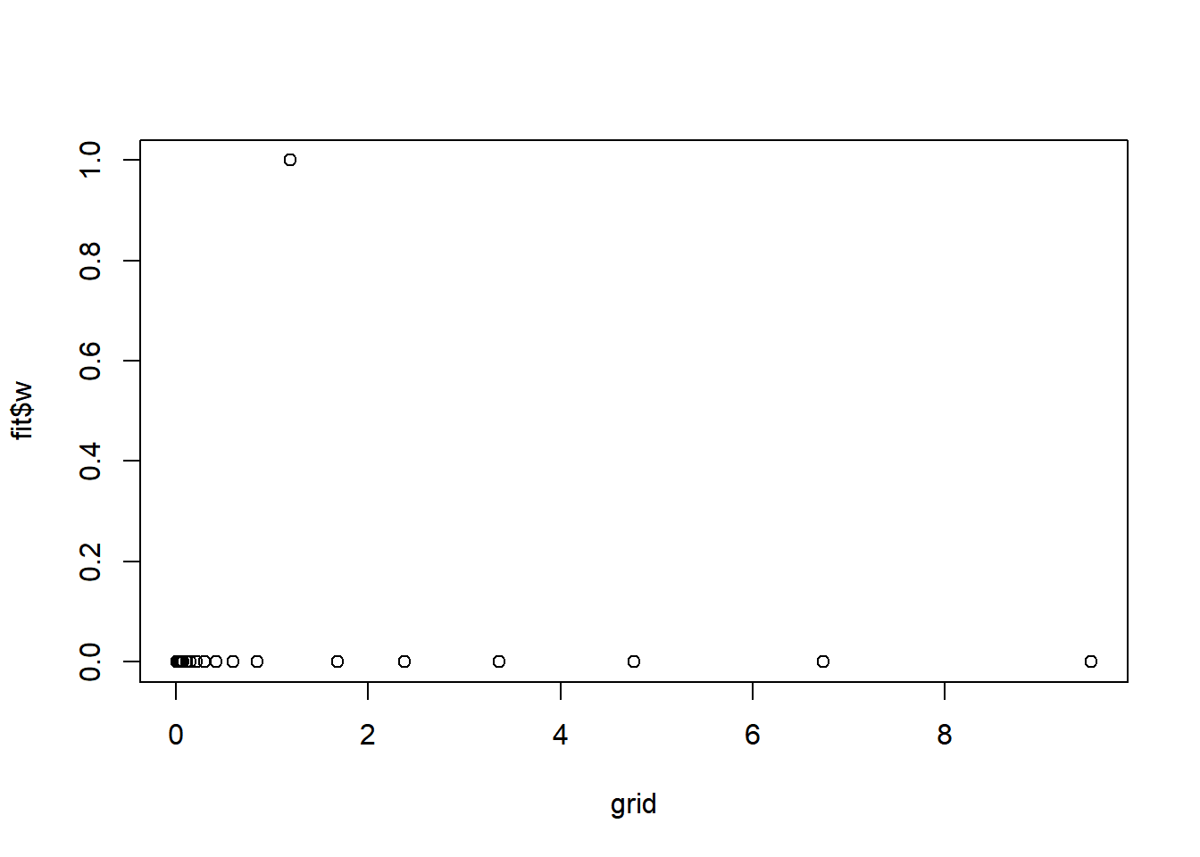

fit$s2

  [1] 1.161368708 0.710919446 1.870311590 1.161368708 1.161368708 0.710919446
  [7] 1.870311588 1.870311588 1.161368708 1.161368708 1.870311592 1.161368708
 [13] 1.161368708 1.870311588 0.475917124 1.161368708 1.870311588 1.161368708
 [19] 1.161368708 1.870311590 1.870311588 1.870311588 1.870311588 1.161368708
 [25] 0.710919446 1.161368708 0.710919446 1.161368708 1.161368708 1.161368708
 [31] 1.870311590 1.161368708 1.161368708 1.161368708 0.710919446 1.161368708
 [37] 0.347687554 0.710919446 1.161368708 1.161368708 0.475917124 0.475917124
 [43] 0.710919446 0.710919446 1.161368708 1.161368708 0.475917124 1.161368708
 [49] 1.870311589 0.710919446 1.870311589 0.475917124 1.870311589 1.870311589
 [55] 0.710919446 0.710919446 1.870311586 1.870311589 1.870311587 1.161368708
 [61] 0.475917124 0.710919446 0.710919446 0.710919446 1.161368708 1.870311590
 [67] 1.870311587 0.710919446 0.347687553 1.161368708 1.870311588 1.870311592
 [73] 1.870311588 0.347687554 0.710919446 1.161368708 1.161368708 1.870311586
 [79] 1.870311586 0.710919446 0.710919446 0.122911972 1.870311586 0.008833582
 [85] 0.475917124 0.022779652 0.347687554 1.161368708 0.270392653 0.710919446
 [91] 1.870311589 1.870311588 0.027743775 1.870311586 1.870311585 1.161368708
 [97] 1.870311586 0.013244965 1.870311586 1.870311588

fit = pois_mean_penalized_nleqslv(x,w=NULL,grid=grid,est_w=TRUE,z_init = log(1+x),opt_method = 'Newton')
plot(L_grad(fit$fit$x,x,grid),ylab='gradient',main='check gradient')

plot(fit$z,col='grey50')
lines(log(1+x),type='p',pch=8,col='grey50')
lines(mu,col='grey80',type='p',pch=20)
lines(fit$m,col=4)
legend('topleft',c('log(1+x)','z','true mu','mu hat'), pch=c(8,1,20,NA),lty=c(NA,NA,NA,1),col=c('grey50','grey50','grey80',4))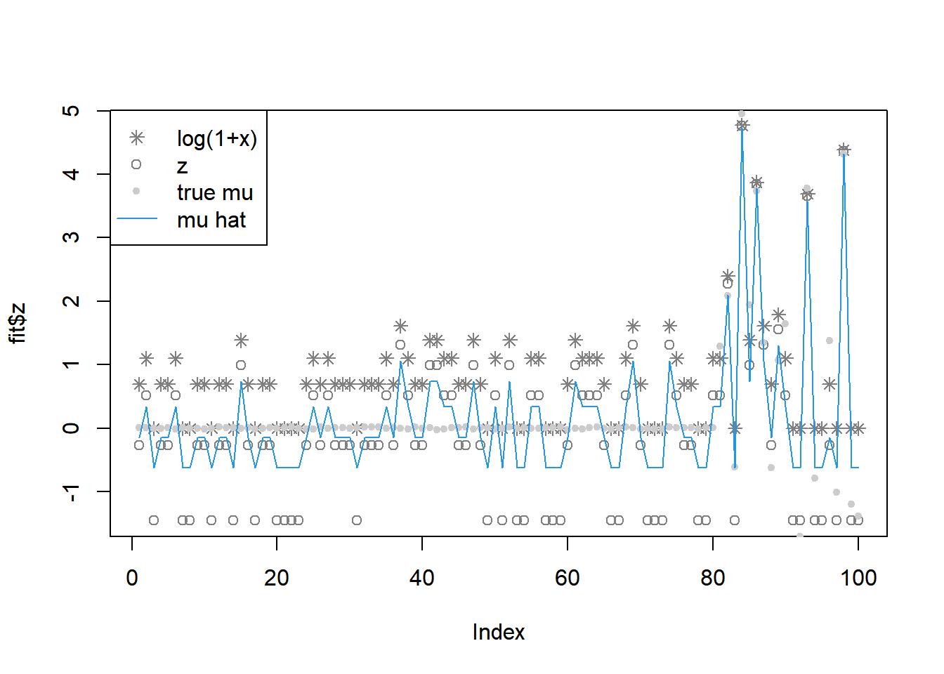

round(fit$w,3)

 [1] 0 0 0 0 0 0 0 0 0 0 0 0 0 0 0 1 0 0 0 0 0 0

plot(grid,fit$w)

fit$s2

  [1] 1.161367355 0.710917648 1.870314513 1.161367354 1.161367354 0.710917648
  [7] 1.870314514 1.870314513 1.161367354 1.161367355 1.870314514 1.161367354
 [13] 1.161367355 1.870314514 0.475927027 1.161367354 1.870314514 1.161367355
 [19] 1.161367354 1.870314512 1.870314515 1.870314513 1.870314512 1.161367354
 [25] 0.710917649 1.161367355 0.710917649 1.161367354 1.161367354 1.161367354
 [31] 1.870314514 1.161367355 1.161367354 1.161367354 0.710917648 1.161367354
 [37] 0.347691536 0.710917648 1.161367355 1.161367354 0.475927027 0.475927027
 [43] 0.710917649 0.710917648 1.161367354 1.161367354 0.475927027 1.161367354
 [49] 1.870314514 0.710917648 1.870314515 0.475927027 1.870314512 1.870314513
 [55] 0.710917648 0.710917648 1.870314514 1.870314513 1.870314513 1.161367354
 [61] 0.475927027 0.710917649 0.710917648 0.710917649 1.161367354 1.870314515
 [67] 1.870314513 0.710917649 0.347691536 1.161367354 1.870314514 1.870314514
 [73] 1.870314515 0.347691536 0.710917649 1.161367354 1.161367354 1.870314514
 [79] 1.870314514 0.710917648 0.710917649 0.122911966 1.870314514 0.008833588
 [85] 0.475927027 0.022779651 0.347691536 1.161367354 0.270393882 0.710917648
 [91] 1.870314514 1.870314516 0.027743770 1.870314515 1.870314512 1.161367354
 [97] 1.870314512 0.013244968 1.870314514 1.870314515

Session information

sessionInfo()

R version 4.2.1 (2022-06-23 ucrt)
Platform: x86_64-w64-mingw32/x64 (64-bit)
Running under: Windows 10 x64 (build 22000)

Matrix products: default

locale:
[1] LC_COLLATE=English_United States.utf8 
[2] LC_CTYPE=English_United States.utf8   
[3] LC_MONETARY=English_United States.utf8
[4] LC_NUMERIC=C                          
[5] LC_TIME=English_United States.utf8    

attached base packages:
[1] stats     graphics  grDevices utils     datasets  methods   base     

other attached packages:
[1] nleqslv_3.3.3   ashr_2.2-54     workflowr_1.7.0

loaded via a namespace (and not attached):
 [1] Rcpp_1.0.9       highr_0.9        compiler_4.2.1   pillar_1.8.1    
 [5] bslib_0.4.0      later_1.3.0      git2r_0.30.1     jquerylib_0.1.4 
 [9] tools_4.2.1      getPass_0.2-2    digest_0.6.29    lattice_0.20-45 
[13] jsonlite_1.8.0   evaluate_0.16    tibble_3.1.8     lifecycle_1.0.2 
[17] pkgconfig_2.0.3  rlang_1.0.5      Matrix_1.4-1     cli_3.3.0       
[21] rstudioapi_0.14  yaml_2.3.5       xfun_0.32        fastmap_1.1.0   
[25] invgamma_1.1     httr_1.4.4       stringr_1.4.1    knitr_1.40      
[29] fs_1.5.2         vctrs_0.4.1      sass_0.4.2       grid_4.2.1      
[33] rprojroot_2.0.3  glue_1.6.2       R6_2.5.1         processx_3.7.0  
[37] fansi_1.0.3      rmarkdown_2.16   mixsqp_0.3-43    irlba_2.3.5     
[41] callr_3.7.2      magrittr_2.0.3   whisker_0.4      ps_1.7.1        
[45] promises_1.2.0.1 htmltools_0.5.3  httpuv_1.6.5     utf8_1.2.2      
[49] stringi_1.7.8    truncnorm_1.0-8  SQUAREM_2021.1   cachem_1.0.6