Overdispersed splitting method dealing with NB data
DongyueXie
2022-11-21
Last updated: 2022-11-21
Checks: 7 0
Knit directory: gsmash/
This reproducible R Markdown analysis was created with workflowr (version 1.7.0). The Checks tab describes the reproducibility checks that were applied when the results were created. The Past versions tab lists the development history.
Great! Since the R Markdown file has been committed to the Git repository, you know the exact version of the code that produced these results.
Great job! The global environment was empty. Objects defined in the global environment can affect the analysis in your R Markdown file in unknown ways. For reproduciblity it’s best to always run the code in an empty environment.
The command set.seed(20220606) was run prior to running
the code in the R Markdown file. Setting a seed ensures that any results
that rely on randomness, e.g. subsampling or permutations, are
reproducible.
Great job! Recording the operating system, R version, and package versions is critical for reproducibility.
Nice! There were no cached chunks for this analysis, so you can be confident that you successfully produced the results during this run.
Great job! Using relative paths to the files within your workflowr project makes it easier to run your code on other machines.
Great! You are using Git for version control. Tracking code development and connecting the code version to the results is critical for reproducibility.
The results in this page were generated with repository version 03048ee. See the Past versions tab to see a history of the changes made to the R Markdown and HTML files.
Note that you need to be careful to ensure that all relevant files for
the analysis have been committed to Git prior to generating the results
(you can use wflow_publish or
wflow_git_commit). workflowr only checks the R Markdown
file, but you know if there are other scripts or data files that it
depends on. Below is the status of the Git repository when the results
were generated:
Ignored files:
    Ignored:    .Rhistory
    Ignored:    .Rproj.user/
    Ignored:    data/poisson_mean_simulation/

Untracked files:
    Untracked:  figure/
    Untracked:  output/poisson_mean_simulation/
    Untracked:  output/poisson_smooth_simulation/

Unstaged changes:
    Modified:   analysis/normal_mean_penalty_glm_simplified.Rmd
    Modified:   code/poisson_mean/simulation_summary.R
Note that any generated files, e.g. HTML, png, CSS, etc., are not included in this status report because it is ok for generated content to have uncommitted changes.
These are the previous versions of the repository in which changes were
made to the R Markdown
(analysis/overdispersed_splitting_nb.Rmd) and HTML
(docs/overdispersed_splitting_nb.html) files. If you’ve
configured a remote Git repository (see ?wflow_git_remote),
click on the hyperlinks in the table below to view the files as they
were in that past version.
| File | Version | Author | Date | Message |
|---|---|---|---|---|
| Rmd | 03048ee | DongyueXie | 2022-11-21 | wflow_publish("analysis/overdispersed_splitting_nb.Rmd") |
Introduction
We simulate mean parameter \(\lambda\) from \(\pi_0\delta_0 + \pi_1Exp(0.1)\).
Then generate data using a NB distribution \(NB(r,p)\). Then \(r(1-p)/p = \lambda\) so \(p = r/(r+\lambda)\). The variance is \(r(1-p)/p^2 = \lambda + \lambda^2/r\).
What’s the corresponding \(\sigma^2\) in \(Poisson(\exp(\mu+\sigma^2))\)?
Since \(\exp(\mu+\sigma2/2)=\lambda\), we have \(\mu = \log\lambda - \sigma^2/2\). Then by matching the variance of NB and the Poisson model, we solve \((\exp(\sigma^2)-1)\exp(2\mu+\sigma^2) = \lambda^2/r\) and we have \(\sigma^2 = \log(1+1/r)\). The smaller the \(r\), the larger oversidpersion.
library(vebpm)r = 10
first run
set.seed(12345)
n = 3000
lambda = c(rep(0,n*0.8),rexp(n*0.2,0.1))
r = 10
y = rnbinom(n,r,mu  = lambda)
sigma2 = log(1+1/r)
sigma2[1] 0.09531018fix \(\sigma2\)
fit = pois_mean_split2(y,sigma2=sigma2,est_sigma2 = FALSE,mu_pm_init = log(y+1))
fit$elbo
[1] -7394.922plot(lambda,col='grey80')
lines(fit$posterior$mean)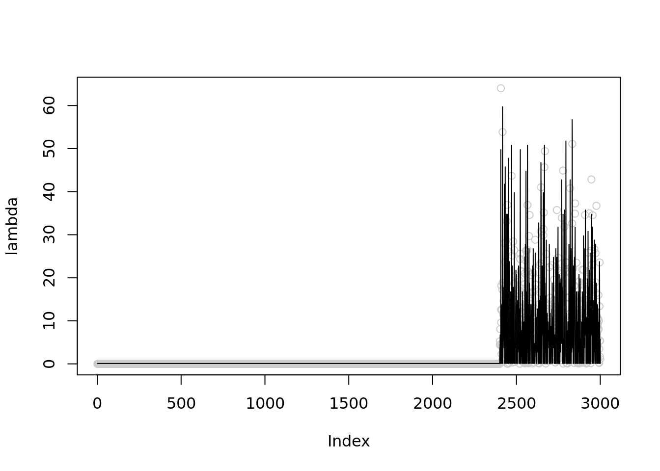
fit$fitted_g$sigma2
[1] 0.09531018
$g_b
$pi
[1] 0.8402475 0.1597525
$mean
[1] -2.315816 -2.315816
$scale
[1] 0.000000 4.057725
attr(,"class")
[1] "laplacemix"
attr(,"row.names")
[1] 1 2second run
lambda = c(rep(0,n*0.8),rexp(n*0.2,0.1))
y = rnbinom(n,r,mu  = lambda)
fix \(\sigma2\)
fit = pois_mean_split2(y,sigma2=sigma2,est_sigma2 = FALSE,mu_pm_init = log(y+1))
fit$elbo
[1] -7463.391plot(lambda,col='grey80')
lines(fit$posterior$mean)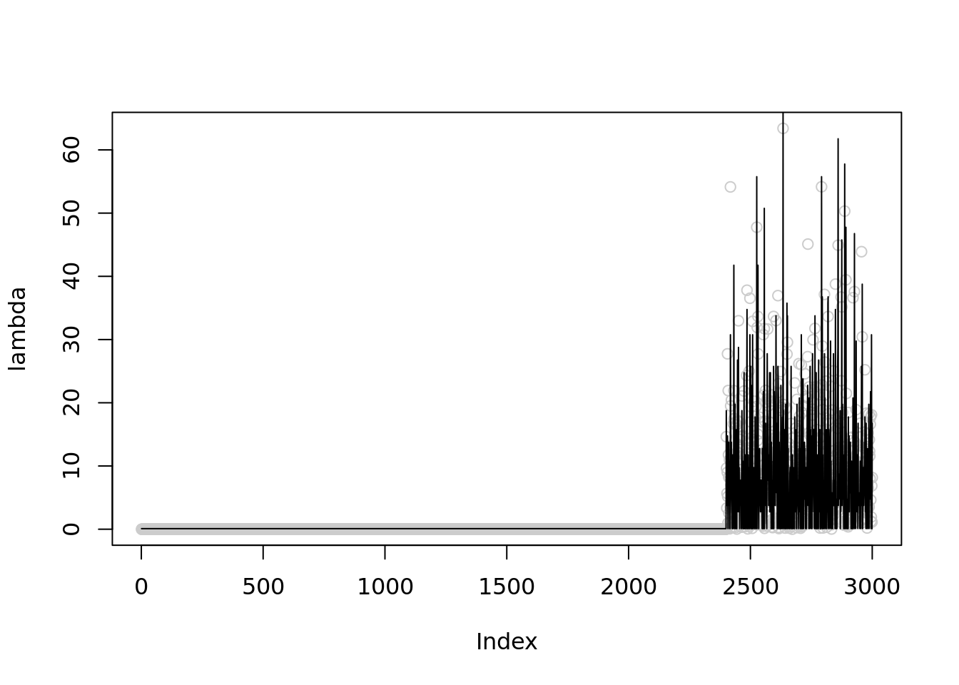
fit$fitted_g$sigma2
[1] 0.09531018
$g_b
$pi
[1] 0.8344718 0.1655282
$mean
[1] -2.403966 -2.403966
$scale
[1] 0.000000 4.176129
attr(,"class")
[1] "laplacemix"
attr(,"row.names")
[1] 1 2third run
lambda = c(rep(0,n*0.8),rexp(n*0.2,0.1))
y = rnbinom(n,r,mu  = lambda)
fix \(\sigma2\)
fit = pois_mean_split2(y,sigma2=sigma2,est_sigma2 = FALSE,mu_pm_init = log(y+1))
fit$elbo
[1] -7394.452plot(lambda,col='grey80')
lines(fit$posterior$mean)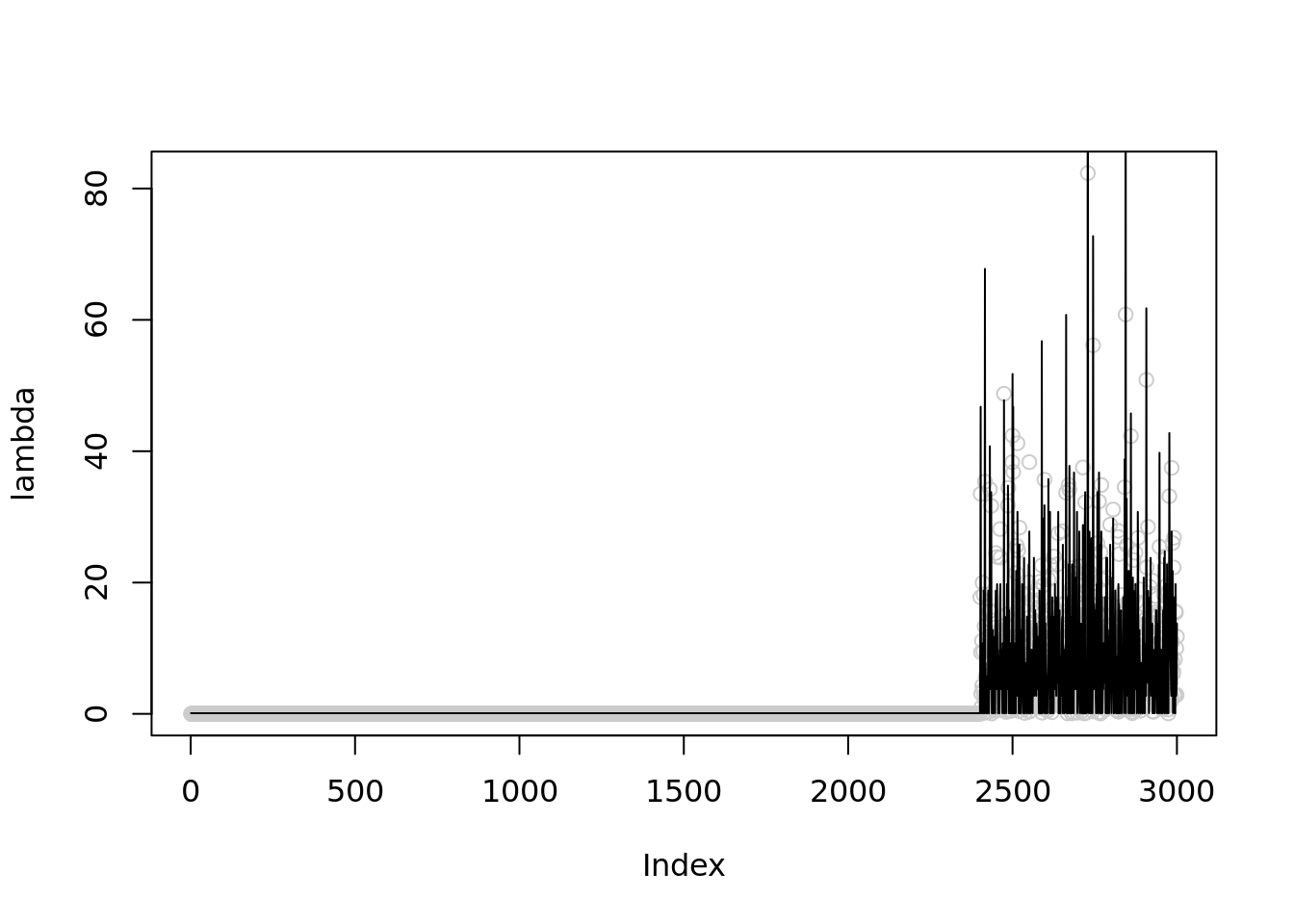
fit$fitted_g$sigma2
[1] 0.09531018
$g_b
$pi
[1] 0.8412745 0.1587255
$mean
[1] -2.332336 -2.332336
$scale
[1] 0.000000 4.137975
attr(,"class")
[1] "laplacemix"
attr(,"row.names")
[1] 1 2r = 5
first run
set.seed(12345)
n = 3000
lambda = c(rep(0,n*0.8),rexp(n*0.2,0.1))
r = 5
y = rnbinom(n,r,mu  = lambda)
sigma2 = log(1+1/r)
sigma2[1] 0.1823216fix \(\sigma2\)
fit = pois_mean_split2(y,sigma2=sigma2,est_sigma2 = FALSE,mu_pm_init = log(y+1))
fit$elbo
[1] -7338.985plot(lambda,col='grey80')
lines(fit$posterior$mean)
fit$fitted_g$sigma2
[1] 0.1823216
$g_b
$pi
[1] 0.8542314 0.1457686
$mean
[1] -1.950497 -1.950497
$scale
[1] 0.000000 3.709187
attr(,"class")
[1] "laplacemix"
attr(,"row.names")
[1] 1 2second run
lambda = c(rep(0,n*0.8),rexp(n*0.2,0.1))
y = rnbinom(n,r,mu  = lambda)
fix \(\sigma2\)
fit = pois_mean_split2(y,sigma2=sigma2,est_sigma2 = FALSE,mu_pm_init = log(y+1))
fit$elbo
[1] -7372.572plot(lambda,col='grey80')
lines(fit$posterior$mean)
fit$fitted_g$sigma2
[1] 0.1823216
$g_b
$pi
[1] 0.8516417 0.1483583
$mean
[1] -1.957995 -1.957995
$scale
[1] 0.000000 3.720176
attr(,"class")
[1] "laplacemix"
attr(,"row.names")
[1] 1 2third run
lambda = c(rep(0,n*0.8),rexp(n*0.2,0.1))

y = rnbinom(n,r,mu  = lambda)
fix \(\sigma2\)
fit = pois_mean_split2(y,sigma2=sigma2,est_sigma2 = FALSE,mu_pm_init = log(y+1))
fit$elbo
[1] -7357.373plot(lambda,col='grey80')
lines(fit$posterior$mean)
fit$fitted_g$sigma2
[1] 0.1823216
$g_b
$pi
[1] 0.8561683 0.1438317
$mean
[1] -1.888776 -1.888776
$scale
[1] 0.000000 3.652401
attr(,"class")
[1] "laplacemix"
attr(,"row.names")
[1] 1 2r = 50
first run
set.seed(12345)
n = 3000
lambda = c(rep(0,n*0.8),rexp(n*0.2,0.1))
r = 50
y = rnbinom(n,r,mu  = lambda)
sigma2 = log(1+1/r)
sigma2[1] 0.01980263fix \(\sigma2\)
fit = pois_mean_split2(y,sigma2=sigma2,est_sigma2 = FALSE,mu_pm_init = log(y+1))Warning in pois_mean_split2(y, sigma2 = sigma2, est_sigma2 = FALSE, mu_pm_init =
log(y + : An iteration decreases ELBO. This is likely due to numerical issues.fit$elbo[1] -11559.26plot(lambda,col='grey80')
lines(fit$posterior$mean)
fit$fitted_g$sigma2
[1] 0.01980263
$g_b
$pi
[1] 0.0004275021 0.9995724979
$mean
[1] -1.222233 -1.222233
$scale
[1] 0.0000000 0.6113245
attr(,"class")
[1] "laplacemix"
attr(,"row.names")
[1] 1 2second run
lambda = c(rep(0,n*0.8),rexp(n*0.2,0.1))

y = rnbinom(n,r,mu  = lambda)
fix \(\sigma2\)
fit = pois_mean_split2(y,sigma2=sigma2,est_sigma2 = FALSE,mu_pm_init = log(y+1))Warning in pois_mean_split2(y, sigma2 = sigma2, est_sigma2 = FALSE, mu_pm_init =
log(y + : An iteration decreases ELBO. This is likely due to numerical issues.fit$elbo[1] -8852.339plot(lambda,col='grey80')
lines(fit$posterior$mean)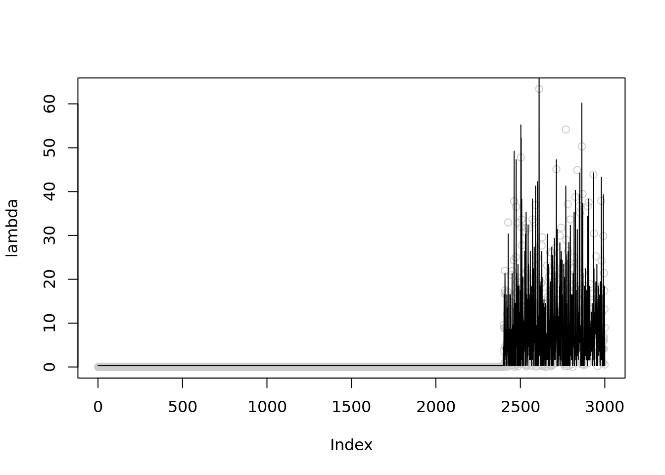
fit$fitted_g$sigma2
[1] 0.01980263
$g_b
$pi
[1] 0.6725263 0.3274737
$mean
[1] -1.216211 -1.216211
$scale
[1] 0.0000000 0.8433485
attr(,"class")
[1] "laplacemix"
attr(,"row.names")
[1] 1 2third run
lambda = c(rep(0,n*0.8),rexp(n*0.2,0.1))

y = rnbinom(n,r,mu  = lambda)
fix \(\sigma2\)
fit = pois_mean_split2(y,sigma2=sigma2,est_sigma2 = FALSE,mu_pm_init = log(y+1))
fit$elbo
[1] -7723.969plot(lambda,col='grey80')
lines(fit$posterior$mean)
fit$fitted_g$sigma2
[1] 0.01980263
$g_b
$pi
[1] 0.831282 0.168718
$mean
[1] -2.427278 -2.427278
$scale
[1] 0.000000 4.317392
attr(,"class")
[1] "laplacemix"
attr(,"row.names")
[1] 1 2r = 500
first run
set.seed(12345)
n = 3000
lambda = c(rep(0,n*0.8),rexp(n*0.2,0.1))
r = 500
y = rnbinom(n,r,mu  = lambda)
sigma2 = log(1+1/r)
sigma2[1] 0.001998003fix \(\sigma2\)
fit = pois_mean_split2(y,sigma2=sigma2,est_sigma2 = FALSE,mu_pm_init = log(y+1))Warning in pois_mean_split2(y, sigma2 = sigma2, est_sigma2 = FALSE, mu_pm_init =
log(y + : An iteration decreases ELBO. This is likely due to numerical issues.fit$elbo[1] -14715.5plot(lambda,col='grey80')
lines(fit$posterior$mean)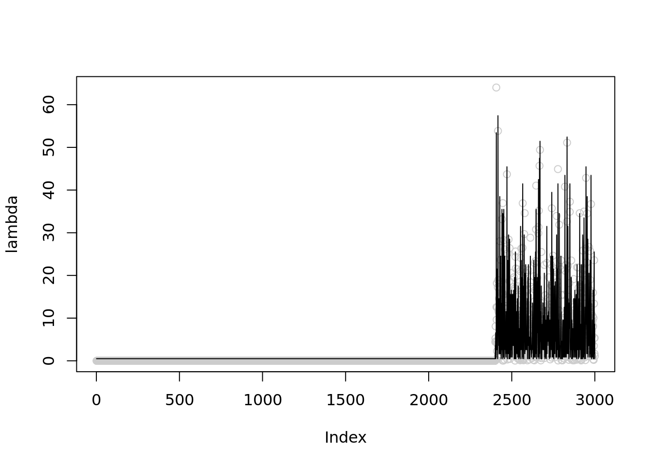
fit$fitted_g$sigma2
[1] 0.001998003
$g_b
$pi
[1] 1.234136e-11 1.000000e+00
$mean
[1] -0.694044 -0.694044
$scale
[1] 0.0000000 0.4826454
attr(,"class")
[1] "laplacemix"
attr(,"row.names")
[1] 1 2second run
lambda = c(rep(0,n*0.8),rexp(n*0.2,0.1))

y = rnbinom(n,r,mu  = lambda)
fix \(\sigma2\)
fit = pois_mean_split2(y,sigma2=sigma2,est_sigma2 = FALSE,mu_pm_init = log(y+1))Warning in pois_mean_split2(y, sigma2 = sigma2, est_sigma2 = FALSE, mu_pm_init =
log(y + : An iteration decreases ELBO. This is likely due to numerical issues.fit$elbo[1] -14951.34plot(lambda,col='grey80')
lines(fit$posterior$mean)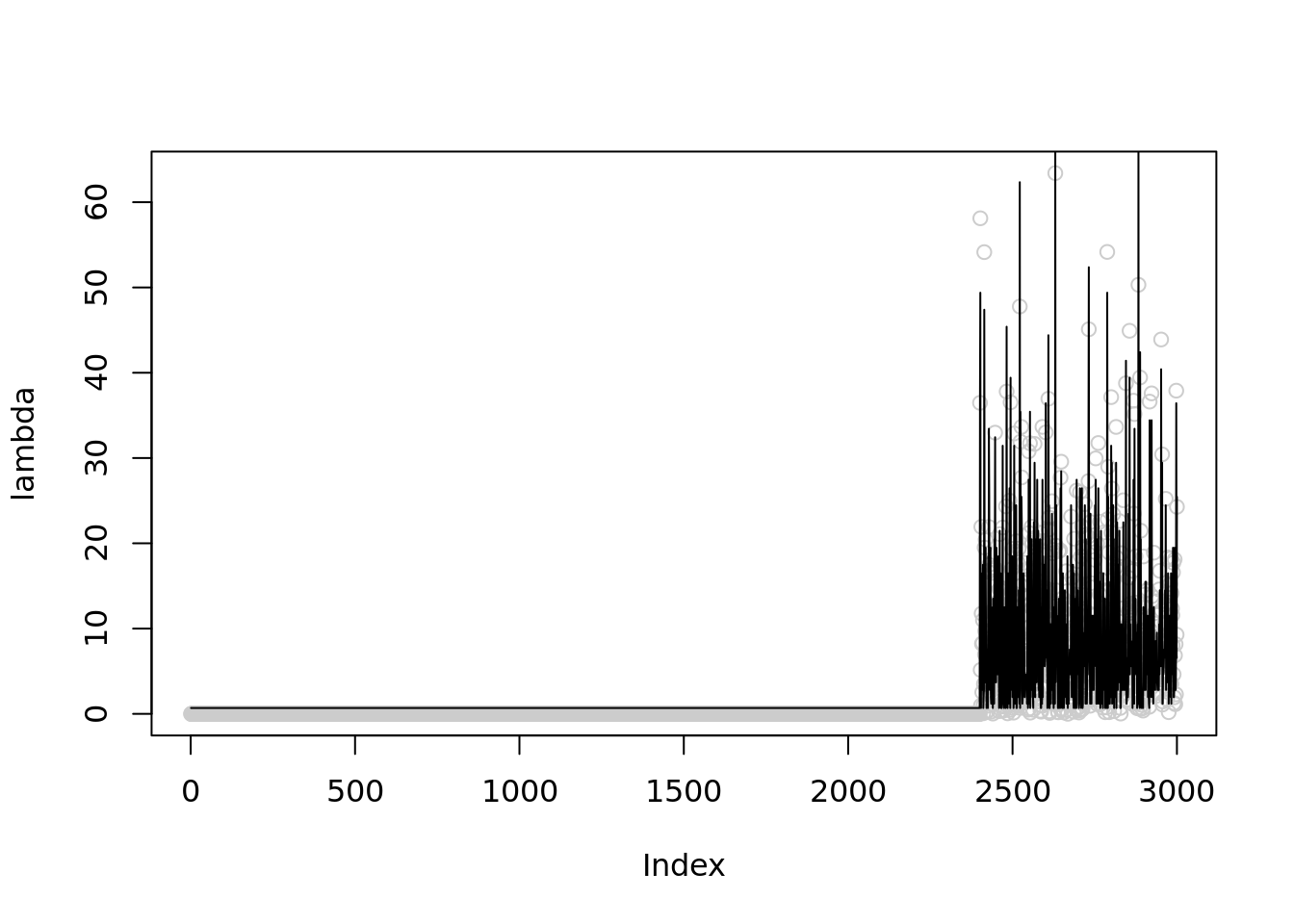
fit$fitted_g$sigma2
[1] 0.001998003
$g_b
$pi
[1] 3.637649e-08 1.000000e+00
$mean
[1] -0.3579676 -0.3579676
$scale
[1] 0.0000000 0.4422295
attr(,"class")
[1] "laplacemix"
attr(,"row.names")
[1] 1 2third run
lambda = c(rep(0,n*0.8),rexp(n*0.2,0.1))

y = rnbinom(n,r,mu  = lambda)
fix \(\sigma2\)
fit = pois_mean_split2(y,sigma2=sigma2,est_sigma2 = FALSE,mu_pm_init = log(y+1))Warning in pois_mean_split2(y, sigma2 = sigma2, est_sigma2 = FALSE, mu_pm_init =
log(y + : An iteration decreases ELBO. This is likely due to numerical issues.fit$elbo[1] -14954.5plot(lambda,col='grey80')
lines(fit$posterior$mean)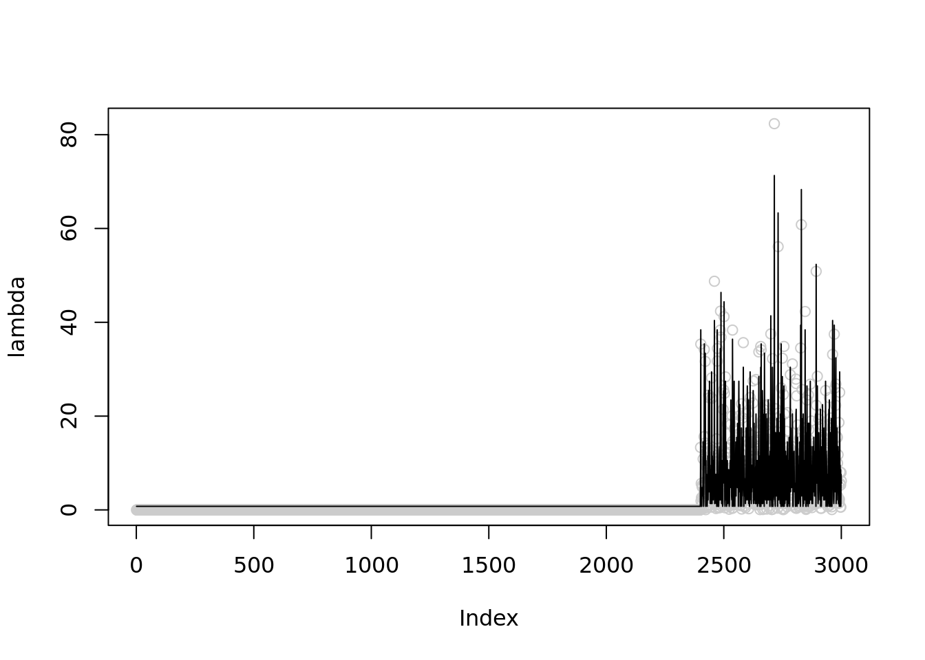
fit$fitted_g$sigma2
[1] 0.001998003
$g_b
$pi
[1] 7.026071e-08 9.999999e-01
$mean
[1] -0.2497244 -0.2497244
$scale
[1] 0.0000000 0.4171243
attr(,"class")
[1] "laplacemix"
attr(,"row.names")
[1] 1 2
sessionInfo()R version 4.2.1 (2022-06-23)
Platform: x86_64-pc-linux-gnu (64-bit)
Running under: Ubuntu 20.04.5 LTS
Matrix products: default
BLAS: /usr/lib/x86_64-linux-gnu/blas/libblas.so.3.9.0
LAPACK: /usr/lib/x86_64-linux-gnu/lapack/liblapack.so.3.9.0
locale:
[1] LC_CTYPE=C.UTF-8 LC_NUMERIC=C LC_TIME=C.UTF-8
[4] LC_COLLATE=C.UTF-8 LC_MONETARY=C.UTF-8 LC_MESSAGES=C.UTF-8
[7] LC_PAPER=C.UTF-8 LC_NAME=C LC_ADDRESS=C
[10] LC_TELEPHONE=C LC_MEASUREMENT=C.UTF-8 LC_IDENTIFICATION=C
attached base packages:
[1] stats graphics grDevices utils datasets methods base
other attached packages:
[1] vebpm_0.2.6 workflowr_1.7.0
loaded via a namespace (and not attached):
[1] Rcpp_1.0.9 horseshoe_0.2.0 invgamma_1.1 lattice_0.20-45
[5] nleqslv_3.3.3 getPass_0.2-2 ps_1.7.1 assertthat_0.2.1
[9] rprojroot_2.0.3 digest_0.6.29 utf8_1.2.2 truncnorm_1.0-8
[13] R6_2.5.1 rootSolve_1.8.2.3 evaluate_0.17 highr_0.9
[17] httr_1.4.4 ggplot2_3.3.6 pillar_1.8.1 rlang_1.0.6
[21] rstudioapi_0.14 ebnm_1.0-9 irlba_2.3.5.1 nloptr_2.0.3
[25] whisker_0.4 callr_3.7.2 jquerylib_0.1.4 Matrix_1.5-1
[29] rmarkdown_2.17 splines_4.2.1 stringr_1.4.1 munsell_0.5.0
[33] mixsqp_0.3-43 compiler_4.2.1 httpuv_1.6.6 xfun_0.33
[37] pkgconfig_2.0.3 SQUAREM_2021.1 htmltools_0.5.3 tidyselect_1.2.0
[41] tibble_3.1.8 matrixStats_0.62.0 fansi_1.0.3 dplyr_1.0.10
[45] later_1.3.0 grid_4.2.1 jsonlite_1.8.2 gtable_0.3.1
[49] lifecycle_1.0.3 DBI_1.1.3 git2r_0.30.1 magrittr_2.0.3
[53] scales_1.2.1 ebpm_0.0.1.3 cli_3.4.1 stringi_1.7.8
[57] cachem_1.0.6 fs_1.5.2 promises_1.2.0.1 bslib_0.4.0
[61] generics_0.1.3 vctrs_0.4.2 trust_0.1-8 tools_4.2.1
[65] glue_1.6.2 parallel_4.2.1 processx_3.7.0 fastmap_1.1.0
[69] yaml_2.3.5 colorspace_2.0-3 ashr_2.2-54 deconvolveR_1.2-1
[73] knitr_1.40 sass_0.4.2