run PMF on pbmc data
DongyueXie
2022-12-06
Last updated: 2022-12-06
Checks: 7 0
Knit directory: gsmash/
This reproducible R Markdown analysis was created with workflowr (version 1.7.0). The Checks tab describes the reproducibility checks that were applied when the results were created. The Past versions tab lists the development history.
Great! Since the R Markdown file has been committed to the Git repository, you know the exact version of the code that produced these results.
Great job! The global environment was empty. Objects defined in the global environment can affect the analysis in your R Markdown file in unknown ways. For reproduciblity it’s best to always run the code in an empty environment.
The command set.seed(20220606) was run prior to running
the code in the R Markdown file. Setting a seed ensures that any results
that rely on randomness, e.g. subsampling or permutations, are
reproducible.
Great job! Recording the operating system, R version, and package versions is critical for reproducibility.
Nice! There were no cached chunks for this analysis, so you can be confident that you successfully produced the results during this run.
Great job! Using relative paths to the files within your workflowr project makes it easier to run your code on other machines.
Great! You are using Git for version control. Tracking code development and connecting the code version to the results is critical for reproducibility.
The results in this page were generated with repository version 39f087b. See the Past versions tab to see a history of the changes made to the R Markdown and HTML files.
Note that you need to be careful to ensure that all relevant files for
the analysis have been committed to Git prior to generating the results
(you can use wflow_publish or
wflow_git_commit). workflowr only checks the R Markdown
file, but you know if there are other scripts or data files that it
depends on. Below is the status of the Git repository when the results
were generated:
Ignored files:
    Ignored:    .Rhistory
    Ignored:    .Rproj.user/
    Ignored:    data/poisson_mean_simulation/

Untracked files:
    Untracked:  code/poisson_STM/plot_factors.R
    Untracked:  code/poisson_STM/real_PMF.R
    Untracked:  figure/
    Untracked:  output/poisson_MF_simulation/
    Untracked:  output/poisson_mean_simulation/
    Untracked:  output/poisson_smooth_simulation/

Unstaged changes:
    Modified:   analysis/index.Rmd
    Modified:   analysis/normal_mean_penalty_glm_simplified.Rmd
    Modified:   analysis/trendfiltering.ipynb
    Modified:   code/poisson_mean/simulation_summary.R
Note that any generated files, e.g. HTML, png, CSS, etc., are not included in this status report because it is ok for generated content to have uncommitted changes.
These are the previous versions of the repository in which changes were
made to the R Markdown (analysis/run_PMF_on_pbmc.Rmd) and
HTML (docs/run_PMF_on_pbmc.html) files. If you’ve
configured a remote Git repository (see ?wflow_git_remote),
click on the hyperlinks in the table below to view the files as they
were in that past version.
| File | Version | Author | Date | Message |
|---|---|---|---|---|
| Rmd | 39f087b | DongyueXie | 2022-12-06 | wflow_publish("analysis/run_PMF_on_pbmc.Rmd") |
Introduction
I take the pbmc data from fastTopics package, and run
splitting PMF on the dataset.
library(fastTopics)
library(Matrix)
library(stm)
Attaching package: 'stm'The following object is masked from 'package:fastTopics':
poisson2multinomdata(pbmc_facs)
counts <- pbmc_facs$counts
table(pbmc_facs$samples$subpop)
 B cell   CD14+   CD34+ NK cell  T cell
    767     163     687     673    1484
## use only B cell and NK cell
cells = pbmc_facs$samples$subpop%in%c('B cell', 'NK cell')
Y = counts[cells,]
dim(Y)[1] 1440 16791# filter out genes that has few expressions(3% cells)
genes = (colSums(Y>0) > 0.03*dim(Y)[1])
Y = Y[,genes]
# make sure there is no zero col and row
sum(rowSums(Y)==0)[1] 0sum(colSums(Y)==0)[1] 0dim(Y)[1] 1440 4015S = tcrossprod(c(rowSums(Y)),c(colSums(Y)))/sum(Y)
Y = as.matrix(Y)There are 5 main cell types and 16791 genes.
To start with, I considered two cell types, B cell, and NK cell. Then I filtered out genes that have no expression in more than \(3\%\) cells. The gene filtering is mainly for reducing the data size and the running time.
The final dataset is of dimension 1440 cells by 4015 genes. I set the
scaling factors as \(s_{ij} =
\frac{y_{i+}y_{+j}}{y_{++}}\). For comparison, I also fit
flash on transformed count data, as \(\tilde{y}_{ij} =
\log(1+\frac{y_{ij}}{s_{ij}}\frac{a_j}{0.5})\) where \(a_j = median(s_{\cdot j})\). This
transformation is derived from \(\tilde{y}_{ij} =
\log(\frac{y_{ij}}{s_{ij}}+\frac{0.5}{a_j})\). However
flash was not able to terminate at \(Kmax = 50\). The splitting PMF estiamted
\(K=3\). In addition, the svd seems to
also support \(K=3\), as the scree plot
show 3 points clearly separated from the rest.
fit = readRDS('output/poisson_MF_simulation/fit_pbmc_2cells.rds')
fit_flashier = readRDS('output/poisson_MF_simulation/fit_flashier_pbmc_2cells.rds')
fit_svd = readRDS('output/poisson_MF_simulation/fit_svd_pbmc_2cells.rds')
plot(fit_svd$d)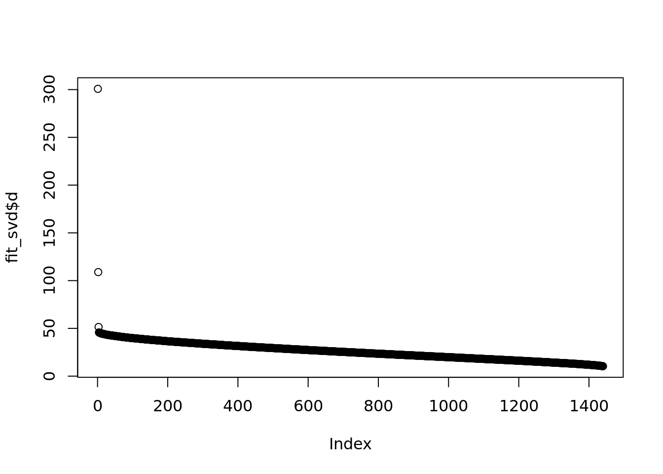
fit$run_timeTime difference of 1.768594 hoursplot(fit$eblo_trace,type='l')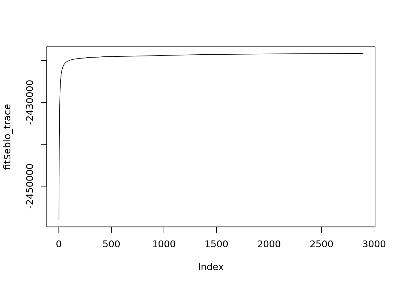
The PMF algorithm converges after \(~3000\) iterations and \(106\)mins.
fit$fit_flash$n.factors[1] 3plot(fit$sigma2,ylab = 'sigma2',xlab='gene',col='grey50')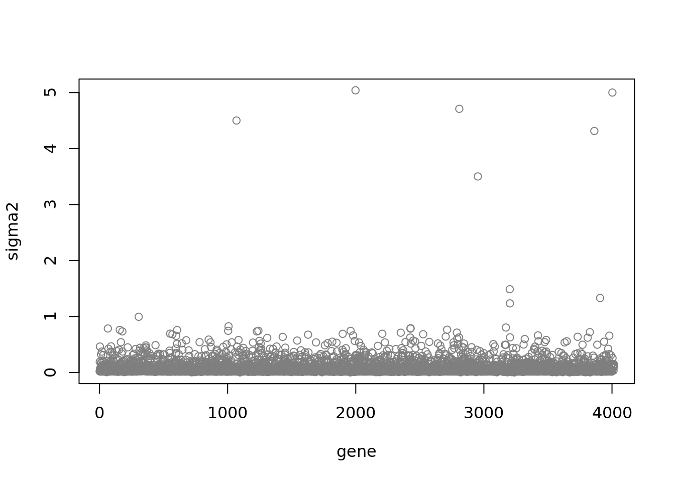
plot(colSums(Y/c(rowSums(Y)))/dim(Y)[1],fit$sigma2,xlab='gene mean count(after library size adjustment)')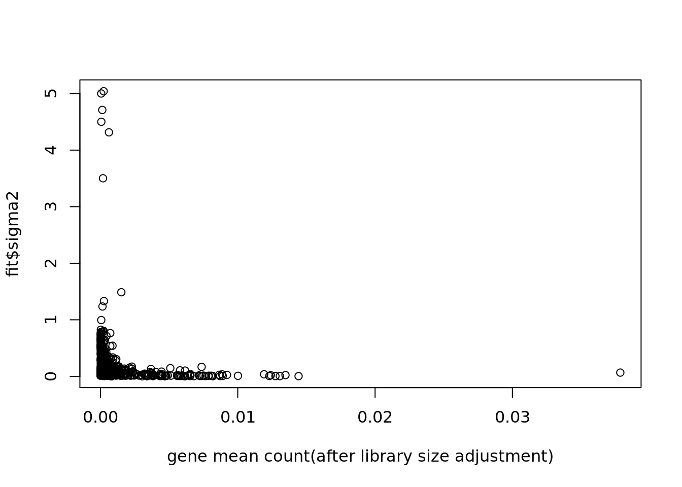
plot(colSums(Y==0)/dim(Y)[1],fit$sigma2,xlab='sparsity')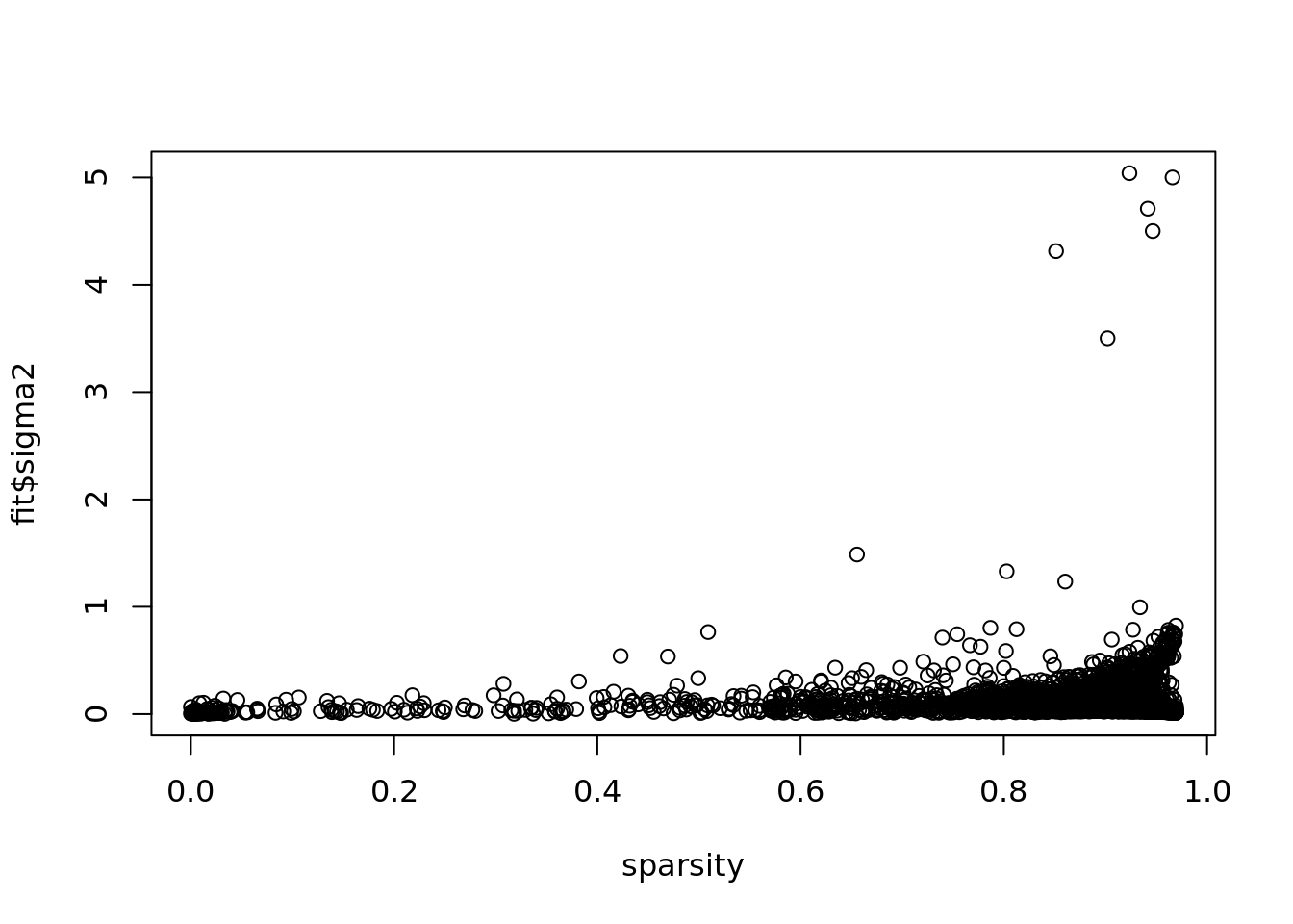
Plot of factors:
par(mfrow=c(3,1))
plot(fit$fit_flash$F.pm[,1],xlab='gene',ylab='first factor')
plot(fit$fit_flash$F.pm[,2],xlab='gene',ylab='second factor')
plot(fit$fit_flash$F.pm[,3],xlab='gene',ylab='third factor')
Plot of Loading:
cell_names = as.character(pbmc_facs$samples$subpop[cells])
color_cell = replace(cell_names,which(cell_names=='B cell'),'red')
color_cell = replace(color_cell,which(cell_names=='NK cell'),'blue')
par(mfrow=c(3,1))
plot(fit$fit_flash$L.pm[,1],xlab='cells',ylab='first loading',col=color_cell)
plot(fit$fit_flash$L.pm[,2],xlab='cells',ylab='second loading',col=color_cell)
plot(fit$fit_flash$L.pm[,3],xlab='cells',ylab='third factor',col=color_cell)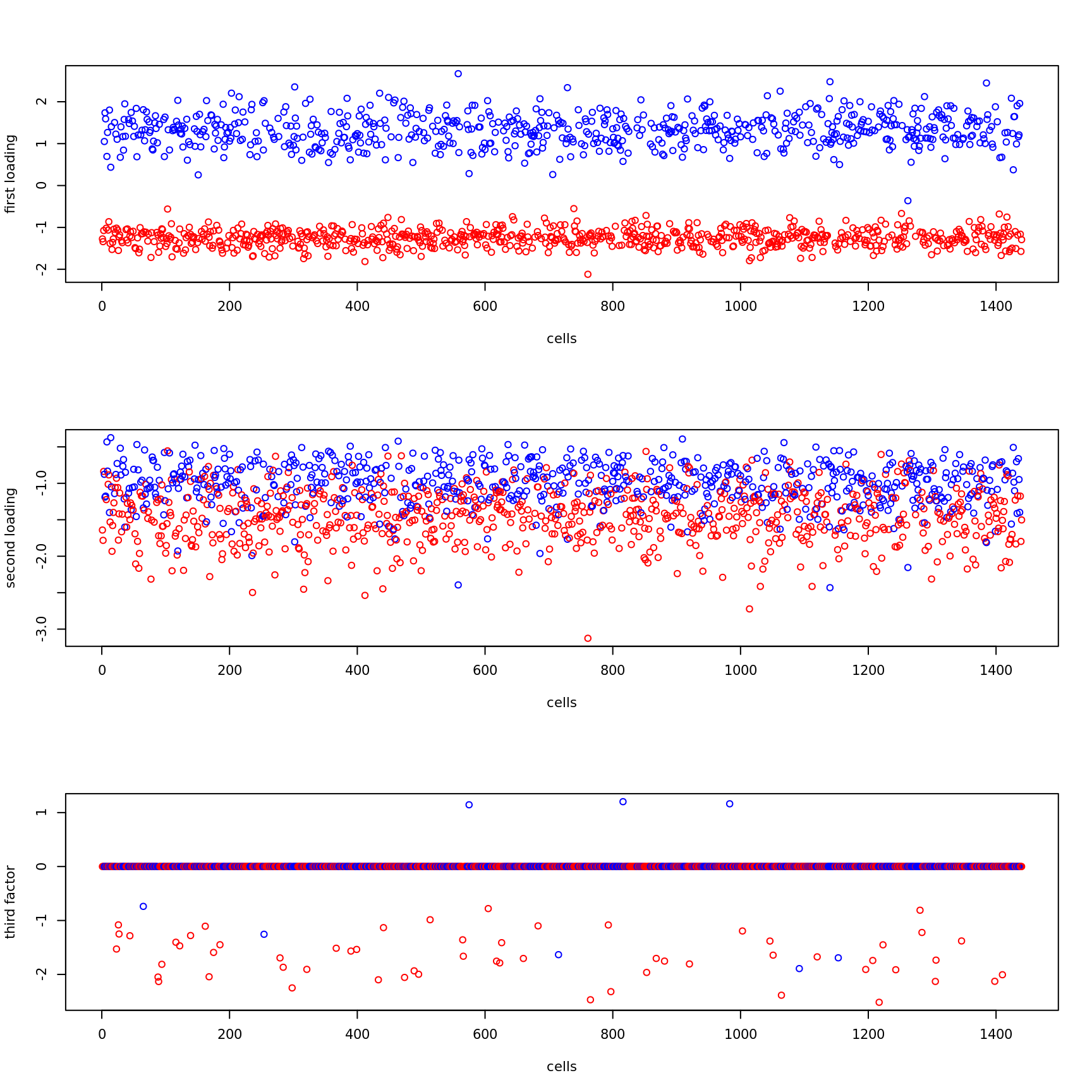
Plot of first two loadings:
par(mfrow=c(1,1))
plot(fit$fit_flash$L.pm[,1],fit$fit_flash$L.pm[,2],col=color_cell,xlab='first loading',ylab='second loading')
legend(c('topright'),c('B cell','NK cell'),col=c('red','blue'),pch=c(1,1))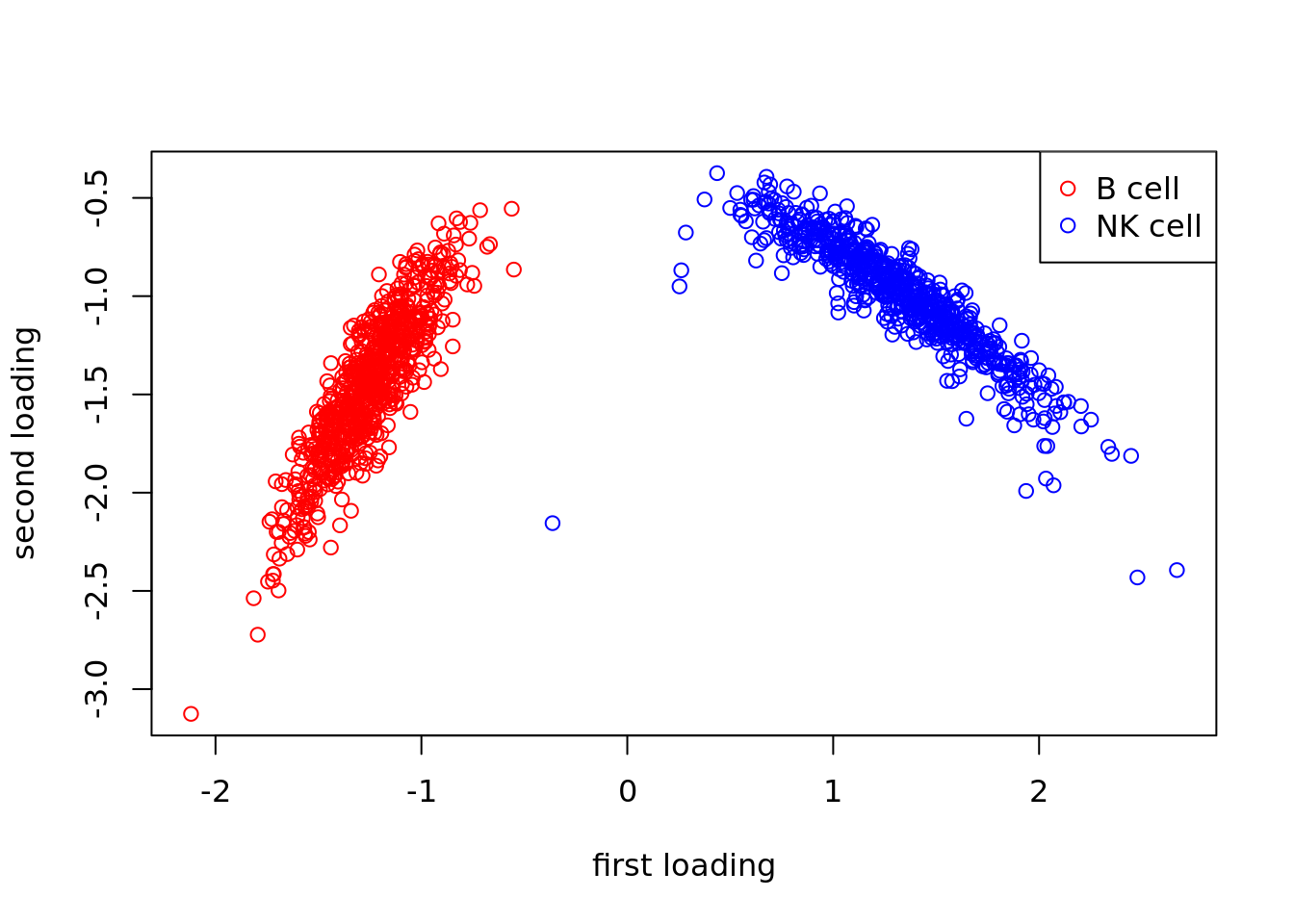
Plot of second two loadings:
par(mfrow=c(1,1))
plot(fit$fit_flash$L.pm[,2],fit$fit_flash$L.pm[,3],col=color_cell,xlab='second loading',ylab='third loading')
legend(c('topleft'),c('B cell','NK cell'),col=c('red','blue'),pch=c(1,1))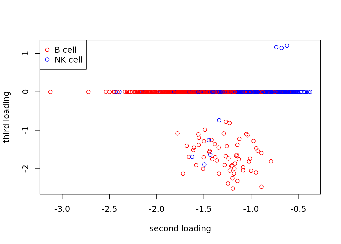
Use Jason’s method for visualizing loadings:
source('code/poisson_STM/plot_factors.R')plot.factors(fit$fit_flash,cell_names,title='splitting PMF')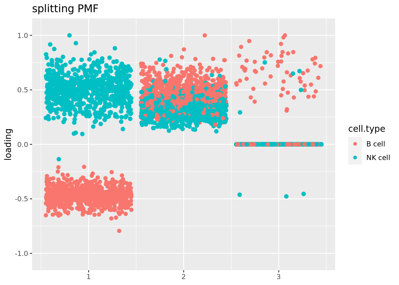
plot.factors(fit_flashier,cell_names,kset = c(1:10),title='flashier')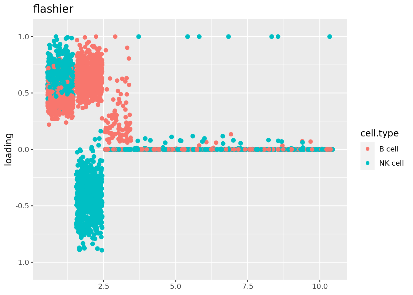
sessionInfo()R version 4.2.1 (2022-06-23)
Platform: x86_64-pc-linux-gnu (64-bit)
Running under: Ubuntu 20.04.5 LTS
Matrix products: default
BLAS: /usr/lib/x86_64-linux-gnu/blas/libblas.so.3.9.0
LAPACK: /usr/lib/x86_64-linux-gnu/lapack/liblapack.so.3.9.0
locale:
[1] LC_CTYPE=C.UTF-8 LC_NUMERIC=C LC_TIME=C.UTF-8
[4] LC_COLLATE=C.UTF-8 LC_MONETARY=C.UTF-8 LC_MESSAGES=C.UTF-8
[7] LC_PAPER=C.UTF-8 LC_NAME=C LC_ADDRESS=C
[10] LC_TELEPHONE=C LC_MEASUREMENT=C.UTF-8 LC_IDENTIFICATION=C
attached base packages:
[1] stats graphics grDevices utils datasets methods base
other attached packages:
[1] ggplot2_3.3.6 stm_1.0.9 Matrix_1.5-1 fastTopics_0.6-142
[5] workflowr_1.7.0
loaded via a namespace (and not attached):
[1] Rtsne_0.16 ebpm_0.0.1.3 colorspace_2.0-3
[4] smashr_1.3-6 ellipsis_0.3.2 rprojroot_2.0.3
[7] fs_1.5.2 rstudioapi_0.14 farver_2.1.1
[10] MatrixModels_0.5-1 ggrepel_0.9.2 fansi_1.0.3
[13] splines_4.2.1 cachem_1.0.6 rootSolve_1.8.2.3
[16] knitr_1.40 jsonlite_1.8.2 nloptr_2.0.3
[19] mcmc_0.9-7 ashr_2.2-54 uwot_0.1.14
[22] compiler_4.2.1 httr_1.4.4 assertthat_0.2.1
[25] fastmap_1.1.0 lazyeval_0.2.2 cli_3.4.1
[28] later_1.3.0 htmltools_0.5.3 quantreg_5.94
[31] prettyunits_1.1.1 tools_4.2.1 coda_0.19-4
[34] gtable_0.3.1 glue_1.6.2 reshape2_1.4.4
[37] dplyr_1.0.10 Rcpp_1.0.9 softImpute_1.4-1
[40] jquerylib_0.1.4 vctrs_0.4.2 wavethresh_4.7.2
[43] xfun_0.33 stringr_1.4.1 ps_1.7.1
[46] trust_0.1-8 lifecycle_1.0.3 irlba_2.3.5.1
[49] NNLM_0.4.4 nleqslv_3.3.3 getPass_0.2-2
[52] MASS_7.3-58 scales_1.2.1 hms_1.1.2
[55] promises_1.2.0.1 parallel_4.2.1 SparseM_1.81
[58] yaml_2.3.5 pbapply_1.6-0 sass_0.4.2
[61] stringi_1.7.8 SQUAREM_2021.1 highr_0.9
[64] deconvolveR_1.2-1 caTools_1.18.2 truncnorm_1.0-8
[67] horseshoe_0.2.0 rlang_1.0.6 pkgconfig_2.0.3
[70] matrixStats_0.62.0 bitops_1.0-7 ebnm_1.0-9
[73] evaluate_0.17 lattice_0.20-45 invgamma_1.1
[76] purrr_0.3.5 htmlwidgets_1.5.4 labeling_0.4.2
[79] cowplot_1.1.1 processx_3.7.0 tidyselect_1.2.0
[82] plyr_1.8.7 magrittr_2.0.3 R6_2.5.1
[85] generics_0.1.3 DBI_1.1.3 pillar_1.8.1
[88] whisker_0.4 withr_2.5.0 survival_3.4-0
[91] mixsqp_0.3-48 tibble_3.1.8 crayon_1.5.2
[94] utf8_1.2.2 plotly_4.10.1 rmarkdown_2.17
[97] progress_1.2.2 grid_4.2.1 data.table_1.14.6
[100] callr_3.7.2 git2r_0.30.1 digest_0.6.29
[103] vebpm_0.3.3 tidyr_1.2.1 httpuv_1.6.6
[106] MCMCpack_1.6-3 RcppParallel_5.1.5 munsell_0.5.0
[109] viridisLite_0.4.1 flashier_0.2.34 bslib_0.4.0
[112] quadprog_1.5-8