Binomial Thinning Ultimate
DongyueXie
2020-03-18
Last updated: 2020-04-01
Checks: 7 0
Knit directory: misc/
This reproducible R Markdown analysis was created with workflowr (version 1.6.0). The Checks tab describes the reproducibility checks that were applied when the results were created. The Past versions tab lists the development history.
Great! Since the R Markdown file has been committed to the Git repository, you know the exact version of the code that produced these results.
Great job! The global environment was empty. Objects defined in the global environment can affect the analysis in your R Markdown file in unknown ways. For reproduciblity it’s best to always run the code in an empty environment.
The command set.seed(20191122) was run prior to running the code in the R Markdown file. Setting a seed ensures that any results that rely on randomness, e.g. subsampling or permutations, are reproducible.
Great job! Recording the operating system, R version, and package versions is critical for reproducibility.
Nice! There were no cached chunks for this analysis, so you can be confident that you successfully produced the results during this run.
Great job! Using relative paths to the files within your workflowr project makes it easier to run your code on other machines.
Great! You are using Git for version control. Tracking code development and connecting the code version to the results is critical for reproducibility. The version displayed above was the version of the Git repository at the time these results were generated.
Note that you need to be careful to ensure that all relevant files for the analysis have been committed to Git prior to generating the results (you can use wflow_publish or wflow_git_commit). workflowr only checks the R Markdown file, but you know if there are other scripts or data files that it depends on. Below is the status of the Git repository when the results were generated:
Ignored files:
    Ignored:    .Rhistory
    Ignored:    .Rproj.user/

Untracked files:
    Untracked:  analysis/contrainedclustering.Rmd
    Untracked:  analysis/gsea.Rmd
    Untracked:  analysis/ideas.Rmd
    Untracked:  analysis/methylation.Rmd
    Untracked:  analysis/susie.Rmd
    Untracked:  code/sccytokines.R
    Untracked:  code/scdeCalibration.R
    Untracked:  data/bart/
    Untracked:  data/cytokine/DE_controls_output_filter10.RData
    Untracked:  data/cytokine/DE_controls_output_filter10_addlimma.RData
    Untracked:  data/cytokine/README
    Untracked:  data/cytokine/test.RData
    Untracked:  data/cytokine_normalized.RData
    Untracked:  data/deconv/
    Untracked:  data/scde/

Unstaged changes:
    Modified:   analysis/CPM.Rmd
    Modified:   analysis/deconvolution.Rmd
    Modified:   analysis/index.Rmd
    Modified:   analysis/limma.Rmd
    Deleted:    data/mout_high.RData
    Deleted:    data/scCDT.RData
    Deleted:    data/sva_sva_high.RData
Note that any generated files, e.g. HTML, png, CSS, etc., are not included in this status report because it is ok for generated content to have uncommitted changes.
These are the previous versions of the R Markdown and HTML files. If you’ve configured a remote Git repository (see ?wflow_git_remote), click on the hyperlinks in the table below to view them.
| File | Version | Author | Date | Message |
|---|---|---|---|---|
| Rmd | 42ee8ca | DongyueXie | 2020-04-01 | wflow_publish(“analysis/binomthinultimate.Rmd”) |
| html | 7177fb2 | DongyueXie | 2020-04-01 | Build site. |
| Rmd | bfa4266 | DongyueXie | 2020-04-01 | wflow_publish(“analysis/binomthinultimate.Rmd”) |
| html | 9576644 | DongyueXie | 2020-03-21 | Build site. |
| Rmd | d6cf110 | DongyueXie | 2020-03-21 | wflow_publish(“analysis/binomthinultimate.Rmd”) |
| html | 9d09fc0 | DongyueXie | 2020-03-21 | Build site. |
| Rmd | c7baf57 | DongyueXie | 2020-03-21 | wflow_publish(“analysis/binomthinultimate.Rmd”) |
I observe that for a real single cell RNA-Seq dataset, if applying binomial thinning, taking log1p, and fitting linear models, then effects with larger standard error tend to be larger. This is seen from the fact that setting \(\alpha=1\) in ash gives higher likelihood than setting \(\alpha=0\). I want to figure out why this happens.
Binomial thinning: given observed counts \(n\) , effect size \(\beta\) and two groups, draw \(y\) either from Binomial\((n, \frac{\exp(\beta)}{1\exp(\beta)})\) or Binomial\((n, \frac{1}{1\exp(\beta)})\), depending on group. Without loss of generality, we assign \(p = \exp(\beta)}{1\exp(\beta)\) to group one and \(1-p\) to group two.
How I tackle this: The standard error of estimated effects is proportional to square root residual variance. Hence, I need to understand the relationship between effects and residual variance. Residual variance is basically \(var(\log(y+s))\), where \(s\) is usually taken to be 0.5 or 1.
Of course, different counts and thinning probabilities result in heterogeneity so a linear model with constant variance is not strictly adequate. Most RUV methods do not consider this heterogeneity. How about voom-ruv-limma-ash combination?
Observed counts vary from 0 to a few hundreds of thousands.
By doing theoretical analysis via Taylor series expansion and extensive simulations, my conclusion is that
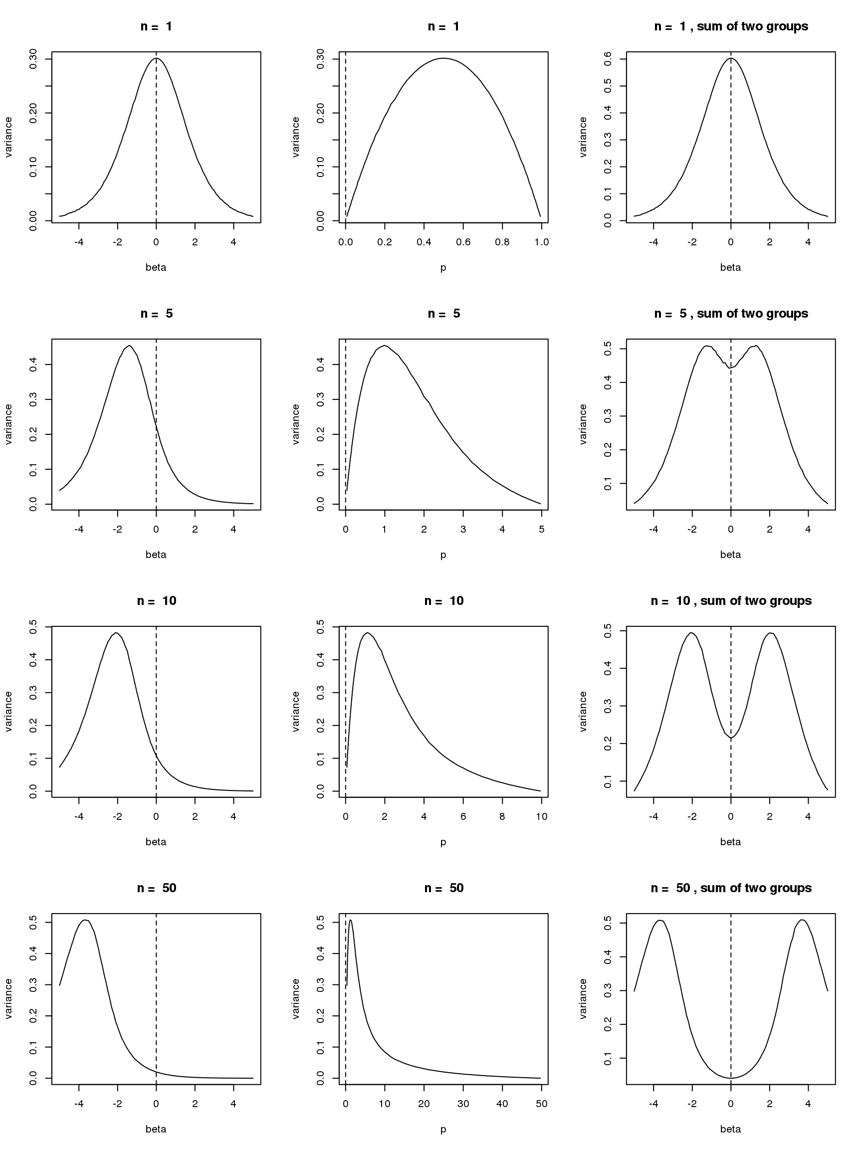
- For group one with \(p=\frac{\exp\beta}{\exp\beta+1}\), \(var(\log(y+s))\) is a unimodal bell shaped function of \(\beta\) given \(n\) and \(s\). Based on first order Taylor series expansion, variance of \(\log(y+s)\) where \(y\sim Binomial(n,\frac{\exp\beta}{1+\exp\beta})\) is \(\frac{n\exp\beta}{((n+s)\exp\beta+s)^2}\), which is maximized at \(\log(\frac{s}{n+s})\). Let’s see some plots for true variance function based on simulating \(10^5\) binomial samples.
Plots on the left in figure below show variance of \(\log(y+0.5)\) vs \(\beta\) relationships for \(n=1,5,10,50\). The ones in the middle change \(\beta\) to \(p\) on x axis. The y axis in right plots are sum of \(var(\log(y+0.5))\) of two groups, i.e. \(var(\log(y_1)+0.5)+var(\log(y_2)+0.5)\), where \(y_1\sim Binomial(n,p)\) and \(y_2\sim Binomial(n,p)\). The idea of these plots are that suppose we have two samples with the same observed counts \(n\) and we assign them to two different groups, we want to understand how total variances(proportional to residual variance) vary with \(\beta\)?
Plots on the left show that as \(n\) goes larger, the \(\beta\) maximizing the curve becomes smaller, which conforms to the Taylor series expansion analysis.
The plots in the middle show that the \(n=1\) curve is similar to a binomial distribution curve(\(p\) vs \(np(1-p)\)) while the other ones skew to right.
library(Biobase)
par(mfrow = c(4,3))

b = seq(-5,5,length.out = 101)
n_list = c(1,5,10,50)
s=0.5

set.seed(12345)

for(n in n_list){
  true_var1 = c()
  true_var2 = c()
  p1 = c()
  p2 = c()
  for(i in 1:length(b)){
    p1[i] = exp(b[i])/(1+exp(b[i]))
    p2[i] = 1/(1+exp(b[i]))
    true_var1 = c(true_var1,var(log(rbinom(1e5,n,p1[i])+s)))
    true_var2 = c(true_var2,var(log(rbinom(1e5,n,p2[i])+s)))
  }

  #print(p1[which.max(true_var1)]*n)

  plot(b,true_var1,type='l',xlab='beta',ylab='variance',main = paste('n = ',n))
  abline(v = 0, lty = 2)

  plot(n*p1,true_var1,type='l',xlab='p',ylab='variance',main = paste('n = ',n))
  abline(v = 0, lty = 2)

  plot(b,true_var1 + true_var2,type='l',xlab='beta',ylab='variance',main = paste('n = ',n, ', sum of two groups'))
  abline(v = 0, lty = 2)
  #plot(p,true_var,type='l')
  # first order taylor series expansion approximated one
  #lines(b, n*exp(b)*(((2*n+2*s+1)*exp(b)+2*s-1)^2+2*(n-1)*exp(b)) / (4*((n+s)*exp(b)+s)^4),col=4)
}
| Version | Author | Date |
|---|---|---|
| 7177fb2 | DongyueXie | 2020-04-01 |
If we consider \(|\beta|\leq 2.5\), then roughly when \(n\geq 15\), \(s.e.(\hat\beta)\) should be monotonically increasing with \(|\beta|\).
load("data/scde/scCDT.RData")
CDT = as.matrix(CDT)
remove.idx = which(rowSums(CDT>0)<=20)
CDT = CDT[-remove.idx,]

#'@param Z count matrix, sample by features
#'@param x 1 for group 1, 0 for group 2
#'@param beta effect of fearures,  0 for null.
#'@return W, thinned matrix
bi_thin = function(Z,x,beta){

  n=nrow(Z)
  p=ncol(Z)

  # group index
  g1 = which(x==1)
  g2 = which(x==0)


  p2 = 1/(1+exp(beta))
  p1 = 1-p2
  P = matrix(nrow = n,ncol = p)
  P[g1,] = t(replicate(length(g1),p1))
  P[g2,] = t(replicate(length(g2),p2))

  W = matrix(rbinom(n*p,Z,P),nrow=n)

  W
}


set.seed(12345)

#beta = sample(seq(-2.5,2.5,length.out = nrow(CDT)))

beta = rnorm(nrow(CDT),0,0.8)

null_idx = sample(1:nrow(CDT),round(0.5*nrow(CDT)))

beta[null_idx] = 0

which_null = 1*(beta==0)

x = rep(0,ncol(CDT))

x[sample(1:ncol(CDT),round(ncol(CDT)/2))] = 1

Y = bi_thin(t(CDT),x,beta)

#Y = Y[,-which(colSums(Y!=0)<10)]

X = model.matrix(~x)

lmout = limma::lmFit(object = t(log(Y+0.5)), design = X)
#eout  <- limma::eBayes(lmout)
out           = list()
out$betahat   = lmout$coefficients[, 2]
out$sebetahat = lmout$stdev.unscaled[, 2] * lmout$sigma
#out$pvalues   = eout$p.value[, 2]

par(mfrow=c(2,2))

plot(beta,out$betahat,ylab='beta_hat')
abline(a=0,b=1)
#plot(abs(beta),out$sebetahat,ylab = 's.e.')
plot(abs(out$betahat),out$sebetahat,xlab = 'abs(beta_hat)',ylab = 's.e.')

alphas = seq(0,1,length.out = 11)

loglik = c()
auc = c()

for(alpha in alphas){
  ash_ash = ashr::ash(out$betahat,out$sebetahat,alpha=alpha)
  loglik = c(loglik,ash_ash$loglik)
  auc = c(auc,pROC::roc(which_null,ash_ash$result$lfsr)$auc)
}

plot(alphas,loglik,type='l',xlab = 'alpha')
plot(alphas,auc,type='l',xlab = 'alpha')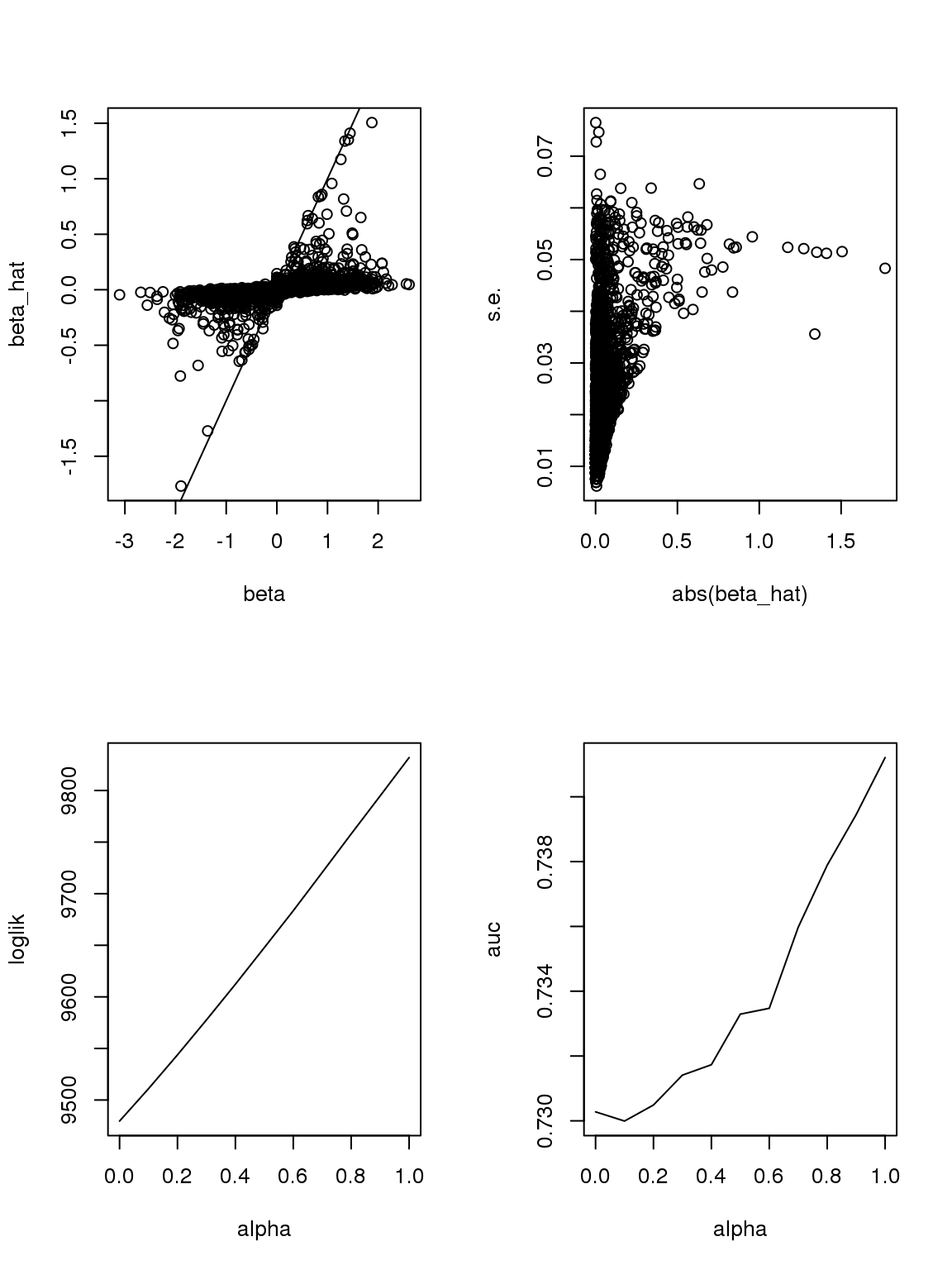
| Version | Author | Date |
|---|---|---|
| 7177fb2 | DongyueXie | 2020-04-01 |
Another run:
#beta = sample(seq(-2.5,2.5,length.out = nrow(CDT)))

beta = rnorm(nrow(CDT),0,0.8)

null_idx = sample(1:nrow(CDT),round(0.5*nrow(CDT)))

beta[null_idx] = 0

which_null = 1*(beta==0)

x = rep(0,ncol(CDT))

x[sample(1:ncol(CDT),round(ncol(CDT)/2))] = 1

Y = bi_thin(t(CDT),x,beta)

#Y = Y[,-which(colSums(Y!=0)<10)]

X = model.matrix(~x)

lmout = limma::lmFit(object = t(log(Y+0.5)), design = X)
#eout  <- limma::eBayes(lmout)
out           = list()
out$betahat   = lmout$coefficients[, 2]
out$sebetahat = lmout$stdev.unscaled[, 2] * lmout$sigma
#out$pvalues   = eout$p.value[, 2]

par(mfrow=c(2,2))

plot(beta,out$betahat,ylab='beta_hat')
abline(a=0,b=1)
#plot(abs(beta),out$sebetahat,ylab = 's.e.')
plot(abs(out$betahat),out$sebetahat,xlab = 'abs(beta_hat)',ylab = 's.e.')

alphas = seq(0,1,length.out = 11)

loglik = c()
auc = c()

for(alpha in alphas){
  ash_ash = ashr::ash(out$betahat,out$sebetahat,alpha=alpha)
  loglik = c(loglik,ash_ash$loglik)
  auc = c(auc,pROC::roc(which_null,ash_ash$result$lfsr)$auc)
}

plot(alphas,loglik,type='l',xlab = 'alpha')
plot(alphas,auc,type='l',xlab = 'alpha')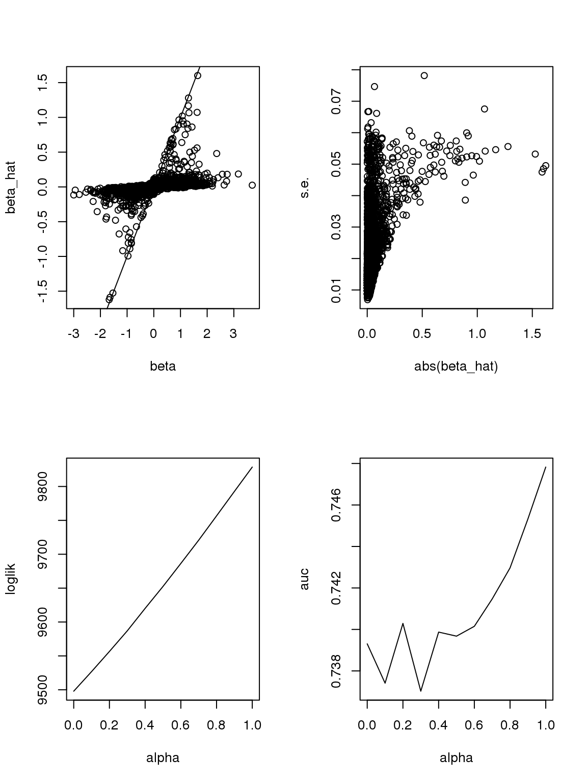
| Version | Author | Date |
|---|---|---|
| 7177fb2 | DongyueXie | 2020-04-01 |
The plot of \(\beta\) vs \(\hat\beta\) shows that if \(\hat\beta\) is large, then \(\beta\) is large. But if \(\beta\) is large, \(\hat\beta\) is not necessarily large because counts are small, the most we can thin is limited. In this sense, some of the ‘true’ \(\beta\)s used to thin the counts are not really ‘true’ since data do not contain such information.
As long as \(\hat\beta\) is a consistent estimator, and sample size is large(701 here, large rnough), \(\hat\beta\) should be close enough to \(\beta\).
However, it seems that the Taylor series and log Binomial analysis still cannot explain the \(\alpha\) stuff. Becuase according to above analysis, since most genes have small counts, then effects with larger s.e. should be smaller. This is certainly not true here. On the other hand, if we only consider genes with maximum counts less or equal to 1, then apply binomial thinning, the results are:
ii = which(rowMax(CDT)<=1)

set.seed(12345)
par(mfrow=c(2,2))

#beta = sample(seq(-2.5,2.5,length.out = nrow(CDT)))

beta = rnorm(nrow(CDT[ii,]),0,0.8)

null_idx = sample(1:nrow(CDT[ii,]),round(0.5*nrow(CDT[ii,])))

beta[null_idx] = 0

which_null = 1*(beta==0)

x = rep(0,ncol(CDT[ii,]))

x[sample(1:ncol(CDT[ii,]),round(ncol(CDT[ii,])/2))] = 1

Y = bi_thin(t(CDT[ii,]),x,beta)

#Y = Y[,-which(colSums(Y!=0)<10)]

X = model.matrix(~x)

lmout = limma::lmFit(object = t(log(Y+0.5)), design = X)
#eout  <- limma::eBayes(lmout)
out           = list()
out$betahat   = lmout$coefficients[, 2]
out$sebetahat = lmout$stdev.unscaled[, 2] * lmout$sigma
#out$pvalues   = eout$p.value[, 2]

plot(beta,out$betahat,ylab='beta_hat')
abline(a=0,b=1)
#plot(abs(beta),out$sebetahat)
plot(abs(out$betahat),out$sebetahat,pch = 18,xlab = 'abs(beta_hat)',ylab = 's.e.')

alphas = seq(0,1,length.out = 11)

loglik = c()
auc = c()

for(alpha in alphas){
  ash_ash = ashr::ash(out$betahat,out$sebetahat,alpha=alpha)
  loglik = c(loglik,ash_ash$loglik)
  auc = c(auc,pROC::roc(which_null,ash_ash$result$lfsr)$auc)
}

plot(alphas,loglik,type='l')
plot(alphas,auc,type='l')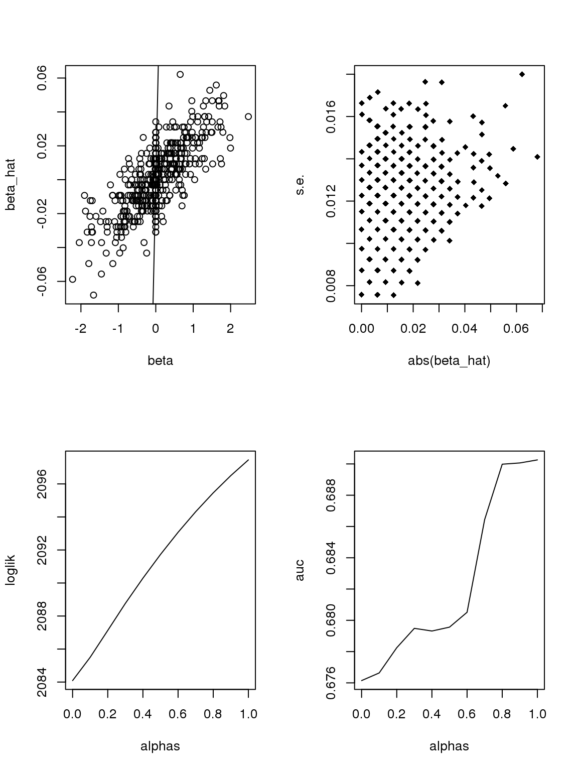
| Version | Author | Date |
|---|---|---|
| 7177fb2 | DongyueXie | 2020-04-01 |
Another run
par(mfrow=c(2,2))
beta = rnorm(nrow(CDT[ii,]),0,0.8)

null_idx = sample(1:nrow(CDT[ii,]),round(0.5*nrow(CDT[ii,])))

beta[null_idx] = 0

which_null = 1*(beta==0)

x = rep(0,ncol(CDT[ii,]))

x[sample(1:ncol(CDT[ii,]),round(ncol(CDT[ii,])/2))] = 1

Y = bi_thin(t(CDT[ii,]),x,beta)

#Y = Y[,-which(colSums(Y!=0)<10)]

X = model.matrix(~x)

lmout = limma::lmFit(object = t(log(Y+0.5)), design = X)
#eout  <- limma::eBayes(lmout)
out           = list()
out$betahat   = lmout$coefficients[, 2]
out$sebetahat = lmout$stdev.unscaled[, 2] * lmout$sigma
#out$pvalues   = eout$p.value[, 2]

plot(beta,out$betahat,ylab='beta_hat')
abline(a=0,b=1)
#plot(abs(beta),out$sebetahat)
plot(abs(out$betahat),out$sebetahat,pch = 18,xlab = 'abs(beta_hat)',ylab = 's.e.')

alphas = seq(0,1,length.out = 11)

loglik = c()
auc = c()

for(alpha in alphas){
  ash_ash = ashr::ash(out$betahat,out$sebetahat,alpha=alpha)
  loglik = c(loglik,ash_ash$loglik)
  auc = c(auc,pROC::roc(which_null,ash_ash$result$lfsr)$auc)
}

plot(alphas,loglik,type='l')
plot(alphas,auc,type='l')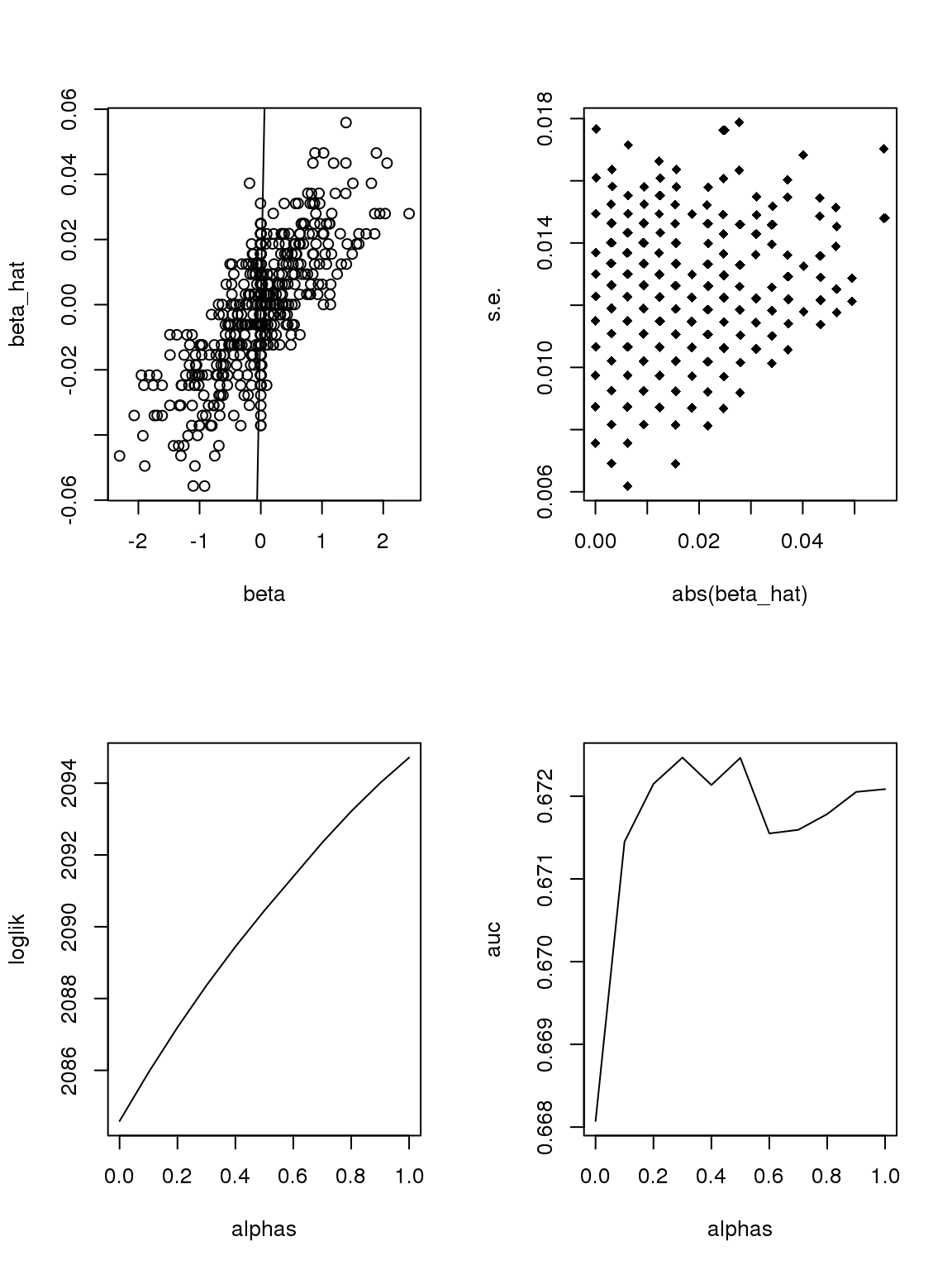
| Version | Author | Date |
|---|---|---|
| 7177fb2 | DongyueXie | 2020-04-01 |
If we only consider genes with maximum counts greater or equal to 50, then apply binomial thinning, the results are:
par(mfrow=c(2,2))
ii = which(rowMax(CDT)>=50)

set.seed(12345)

#beta = sample(seq(-2.5,2.5,length.out = nrow(CDT)))

beta = rnorm(nrow(CDT[ii,]),0,0.8)

null_idx = sample(1:nrow(CDT[ii,]),round(0.5*nrow(CDT[ii,])))

beta[null_idx] = 0

which_null = 1*(beta==0)

x = rep(0,ncol(CDT[ii,]))

x[sample(1:ncol(CDT[ii,]),round(ncol(CDT[ii,])/2))] = 1

Y = bi_thin(t(CDT[ii,]),x,beta)

#Y = Y[,-which(colSums(Y!=0)<10)]

X = model.matrix(~x)

lmout = limma::lmFit(object = t(log(Y+0.5)), design = X)
#eout  <- limma::eBayes(lmout)
out           = list()
out$betahat   = lmout$coefficients[, 2]
out$sebetahat = lmout$stdev.unscaled[, 2] * lmout$sigma
#out$pvalues   = eout$p.value[, 2]

plot(beta,out$betahat,ylab='beta_hat')
abline(a=0,b=1)
#plot(abs(beta),out$sebetahat)
plot(abs(out$betahat),out$sebetahat,pch = 18,xlab = 'abs(beta_hat)',ylab = 's.e.')

alphas = seq(0,1,length.out = 11)

loglik = c()
auc = c()

for(alpha in alphas){
  ash_ash = ashr::ash(out$betahat,out$sebetahat,alpha=alpha)
  loglik = c(loglik,ash_ash$loglik)
  auc = c(auc,pROC::roc(which_null,ash_ash$result$lfsr)$auc)
}

plot(alphas,loglik,type='l')
plot(alphas,auc,type='l')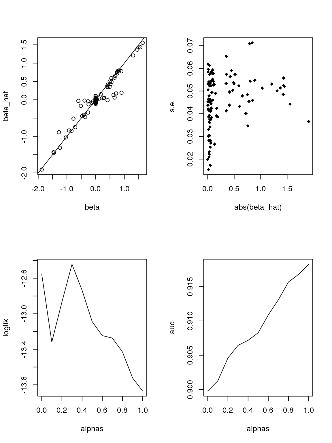
| Version | Author | Date |
|---|---|---|
| 7177fb2 | DongyueXie | 2020-04-01 |
Another run
par(mfrow=c(2,2))
beta = rnorm(nrow(CDT[ii,]),0,0.8)

null_idx = sample(1:nrow(CDT[ii,]),round(0.5*nrow(CDT[ii,])))

beta[null_idx] = 0

which_null = 1*(beta==0)

x = rep(0,ncol(CDT[ii,]))

x[sample(1:ncol(CDT[ii,]),round(ncol(CDT[ii,])/2))] = 1

Y = bi_thin(t(CDT[ii,]),x,beta)

#Y = Y[,-which(colSums(Y!=0)<10)]

X = model.matrix(~x)

lmout = limma::lmFit(object = t(log(Y+0.5)), design = X)
#eout  <- limma::eBayes(lmout)
out           = list()
out$betahat   = lmout$coefficients[, 2]
out$sebetahat = lmout$stdev.unscaled[, 2] * lmout$sigma
#out$pvalues   = eout$p.value[, 2]

plot(beta,out$betahat,ylab='beta_hat')
abline(a=0,b=1)
#plot(abs(beta),out$sebetahat)
plot(abs(out$betahat),out$sebetahat,pch = 18,xlab = 'abs(beta_hat)',ylab = 's.e.')

alphas = seq(0,1,length.out = 11)

loglik = c()
auc = c()

for(alpha in alphas){
  ash_ash = ashr::ash(out$betahat,out$sebetahat,alpha=alpha)
  loglik = c(loglik,ash_ash$loglik)
  auc = c(auc,pROC::roc(which_null,ash_ash$result$lfsr)$auc)
}

plot(alphas,loglik,type='l')
plot(alphas,auc,type='l')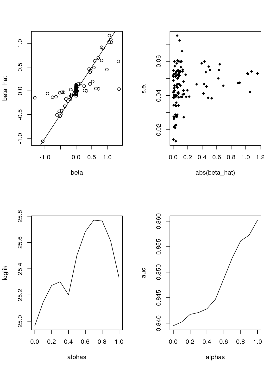
| Version | Author | Date |
|---|---|---|
| 7177fb2 | DongyueXie | 2020-04-01 |
So there must have something to do with the 0’s.
Let’s directly work with \(\hat{\sigma}^2\),
\[\begin{equation} \hat{\sigma}^2 = \frac{1}{n-2}(\sum_{i\in Group1}(y_i-\bar{y}_1)^2+\sum_{i\in Group2}(y_i-\bar{y}_2)^2), \end{equation}\]where \(\bar{y}_1\) is the sample mean of group 1. Let \(n_1\) be the number of samples in group, \(p_1^0\) be the proportion of zeros or \(\log(s)\) in group 1, and \(y_0\) denote zero or \(\log(s)\), then
\[\begin{equation} \begin{split} \sum_{i\in Group1}(y_i-\bar{y}_1)^2 &= \sum_{\substack{i\in Group1 \\ y_i\neq y_0}}(y_i-\bar{y}_1)^2 + n_1p_1^0(y_0-\bar{y}_1)^2 \\&= \sum_{\substack{i\in Group1 \\ y_i\neq y_0}} y_i ^2 - 2p_1^0y_0\sum_{\substack{i\in Group1 \\ y_i\neq y_0}} y_i - \frac{1}{n_1}(\sum_{\substack{i\in Group1 \\ y_i\neq y_0}} y_i)^2 + n_1 p_1^0(1-p_1^0)y_0^2 \\&= n_1(1-p_1^0)\text{Var}\{y_i,\in Group1, y_i\neq y_0\} + \frac{(\sum_{\substack{i\in Group1 \\ y_i\neq y_0}} y_i)^2}{n_1/p_1^0-n_1} + n_1 p_1^0(1-p_1^0)y_0(y_0-2\bar{y}_{1,y_i\neq y_0}) \end{split} \end{equation}\]G=1000
n=100
Y = matrix(0,nrow=G,ncol=n)
Y = t(Y)
Y[1:10,] = 1
Y[51:60,] = 1
Y = t(Y)
set.seed(12345)
beta = rnorm(G,0,0.8)
null_idx = sample(1:G,round(0.5*G))
beta[null_idx] = 0
which_null = 1*(beta==0)
x = rep(0,n)
x[sample(1:n,round(n/2))] = 1
Y = bi_thin(t(Y),x,beta)
#Y = Y[,-which(colSums(Y!=0)<10)]
X = model.matrix(~x)
lmout = limma::lmFit(object = t(log(Y+0.5)), design = X)
#eout <- limma::eBayes(lmout)
out = list()
out$betahat = lmout$coefficients[, 2]
out$sebetahat = lmout$stdev.unscaled[, 2] * lmout$sigma
#out$pvalues = eout$p.value[, 2]
plot(beta,out$betahat,ylab='beta_hat')
abline(a=0,b=1)
#plot(abs(beta),out$sebetahat)
plot((out$betahat),out$sebetahat,pch = 18,xlab = '(beta_hat)',ylab = 's.e.')
alphas = seq(0,1,length.out = 11)
loglik = c()
auc = c()
for(alpha in alphas){
ash_ash = ashr::ash(out$betahat,out$sebetahat,alpha=alpha)
loglik = c(loglik,ash_ash$loglik)
auc = c(auc,pROC::roc(which_null,ash_ash$result$lfsr)$auc)
}
plot(alphas,loglik,type='l')
plot(alphas,auc,type='l')G=1000
n=100
Y = matrix(0,nrow=G,ncol=n)
Y = t(Y)
Y[1:5,] = 1
Y[6:10,] = 50
Y[51:55,] = 1
Y[56:60,] = 1
Y = t(Y)
set.seed(12345)
beta = rnorm(G,0,0.8)
null_idx = sample(1:G,round(0.5*G))
beta[null_idx] = 0
which_null = 1*(beta==0)
x = rep(0,n)
x[sample(1:n,round(n/2))] = 1
Y = bi_thin(t(Y),x,beta)
#Y = Y[,-which(colSums(Y!=0)<10)]
X = model.matrix(~x)
lmout = limma::lmFit(object = t(log(Y+0.5)), design = X)
#eout <- limma::eBayes(lmout)
out = list()
out$betahat = lmout$coefficients[, 2]
out$sebetahat = lmout$stdev.unscaled[, 2] * lmout$sigma
#out$pvalues = eout$p.value[, 2]
plot(beta,out$betahat,ylab='beta_hat')
abline(a=0,b=1)
#plot(abs(beta),out$sebetahat)
plot((out$betahat),out$sebetahat,pch = 18,xlab = '(beta_hat)',ylab = 's.e.')
alphas = seq(0,1,length.out = 11)
loglik = c()
auc = c()
for(alpha in alphas){
ash_ash = ashr::ash(out$betahat,out$sebetahat,alpha=alpha)
loglik = c(loglik,ash_ash$loglik)
auc = c(auc,pROC::roc(which_null,ash_ash$result$lfsr)$auc)
}
plot(alphas,loglik,type='l')
plot(alphas,auc,type='l')Earlier analysis
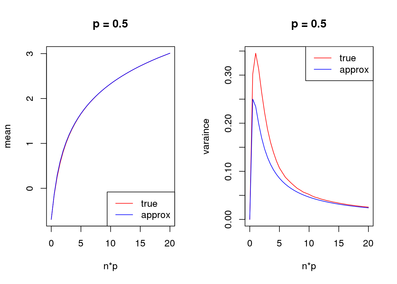
Taylor series approximation
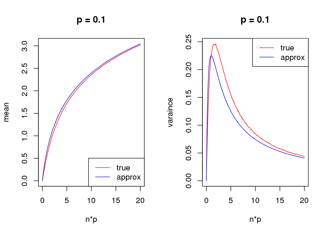
First order
mean_log = function(n,p,s){
  log(n*p+s)
}

var_log = function(n,p,s){
  n*p*(1-p)/(n*p+s)^2
}


s = 1


  set.seed(12345)

  for(p in c(0.1,0.5,0.9)){

  true_var = c()
  approx_var = c()

  true_mean = c()
  approx_mean = c()

  n_list = 0:ceiling(20/p)
  for(n in n_list){
    y = rbinom(1e5,n,p)
    true_var = c(true_var,var(log(y+s)))
    true_mean = c(true_mean,mean(log(y+s)))
    approx_var = c(approx_var,var_log(n,p,s))
    approx_mean = c(approx_mean,mean_log(n,p,s))
  }

  par(mfrow = c(1,2))

  plot(n_list*p,true_mean,type='l',col=2,xlab = 'n*p',ylab = 'mean',ylim = range(c(true_mean,approx_mean)),main = paste('p =',p))
  lines(n_list*p,approx_mean,col=4)
  legend('bottomright',c('true','approx'),lty=c(1,1),col=c(2,4))

  plot(n_list*p,true_var,type='l',col=2,xlab = 'n*p',ylab = 'varaince',ylim = range(c(true_var,approx_var)),main = paste('p =',p))
  lines(n_list*p,approx_var,col=4)
  legend('topright',c('true','approx'),lty=c(1,1),col=c(2,4))

}
| Version | Author | Date |
|---|---|---|
| 7177fb2 | DongyueXie | 2020-04-01 |
| Version | Author | Date |
|---|---|---|
| 7177fb2 | DongyueXie | 2020-04-01 |
| Version | Author | Date |
|---|---|---|
| 7177fb2 | DongyueXie | 2020-04-01 |
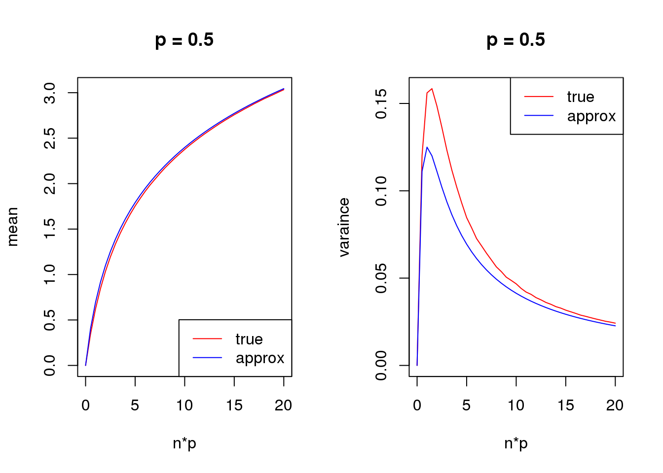
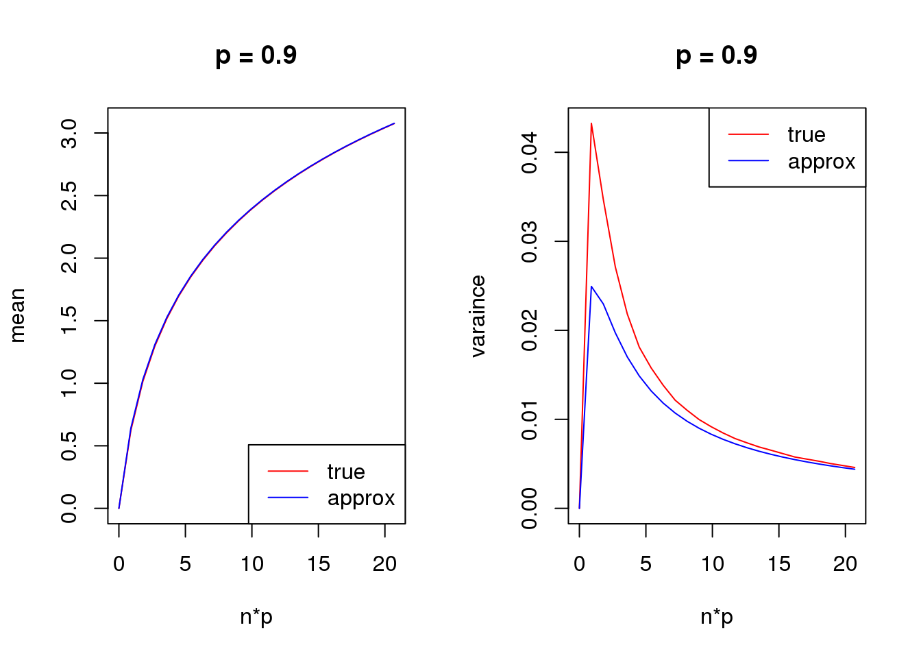
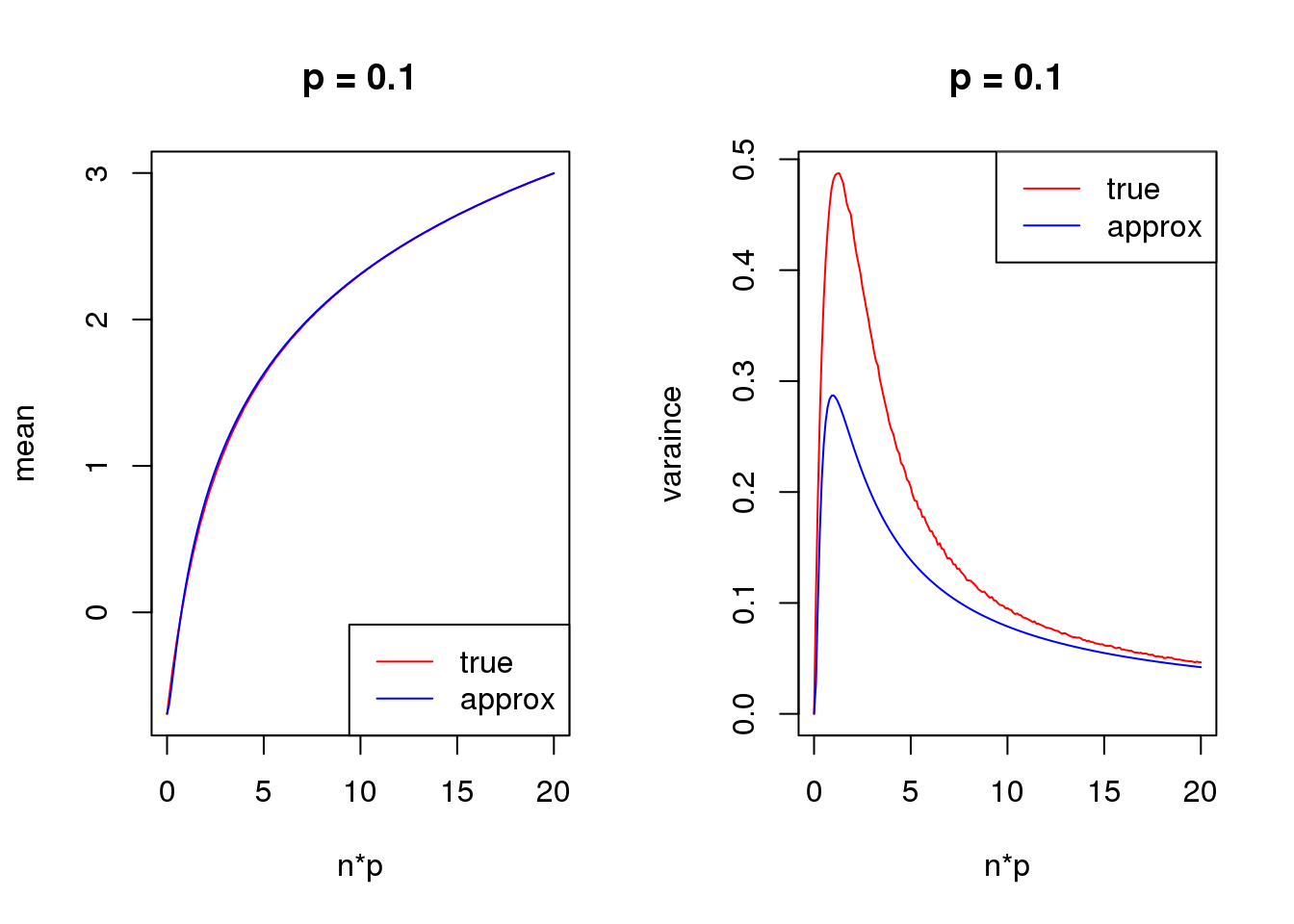
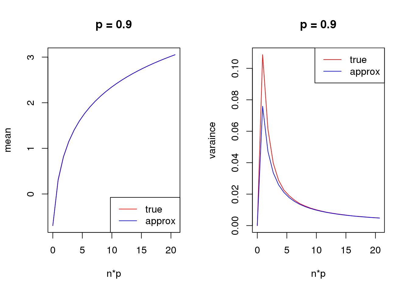
Second order
mean_log = function(n,p,s){
  log(n*p+s)-n*p*(1-p)/(2*(n*p+s)^2)
}

var_log = function(n,p,s){
  n*p*(1-p)/(n*p+s)^2 + n*p*(1-p)*(1+(2*n-6)*p*(1-p))/(4*(n*p+s)^4) - n*p*(1-p)*(1-2*p)/(n*p+s)^3
}


s = 0.5


  set.seed(12345)

  for(p in c(0.1,0.5,0.9)){

  true_var = c()
  approx_var = c()

  true_mean = c()
  approx_mean = c()

  n_list = 0:ceiling(20/p)
  for(n in n_list){
    y = rbinom(1e5,n,p)
    true_var = c(true_var,var(log(y+s)))
    true_mean = c(true_mean,mean(log(y+s)))
    approx_var = c(approx_var,var_log(n,p,s))
    approx_mean = c(approx_mean,mean_log(n,p,s))
  }

  par(mfrow = c(1,2))

  plot(n_list*p,true_mean,type='l',col=2,xlab = 'n*p',ylab = 'mean',ylim = range(c(true_mean,approx_mean)),main = paste('p =',p))
  lines(n_list*p,approx_mean,col=4)
  legend('bottomright',c('true','approx'),lty=c(1,1),col=c(2,4))

  plot(n_list*p,true_var,type='l',col=2,xlab = 'n*p',ylab = 'varaince',ylim = range(c(true_var,approx_var)),main = paste('p =',p))
  lines(n_list*p,approx_var,col=4)
  legend('topright',c('true','approx'),lty=c(1,1),col=c(2,4))

}
| Version | Author | Date |
|---|---|---|
| 7177fb2 | DongyueXie | 2020-04-01 |
| Version | Author | Date |
|---|---|---|
| 7177fb2 | DongyueXie | 2020-04-01 |
| Version | Author | Date |
|---|---|---|
| 7177fb2 | DongyueXie | 2020-04-01 |
Large \(np\)
set.seed(12345)
p_list = seq(0.1,0.5,length.out = 100)

n = 50
s = 0.5


true_var = c()
approx_var = c()

for(p in p_list){
  y1 = rbinom(1e5,n,p)
  y2 = rbinom(1e5,n,1-p)
  true_var = c(true_var,var(log(y1+s))+var(log(y2+s)))
  approx_var = c(approx_var,var_log(n,p,s)+var_log(n,1-p,s))
}

par(mfrow=c(1,1))

plot(log(1/p_list-1),true_var,xlab = 'beta', ylab= 'variance',type='l',col=2,ylim = range(c(true_var,approx_var)))
lines(log(1/p_list-1),approx_var,col=4)
legend('topleft',c('true','approx'),lty=c(1,1),col=c(2,4))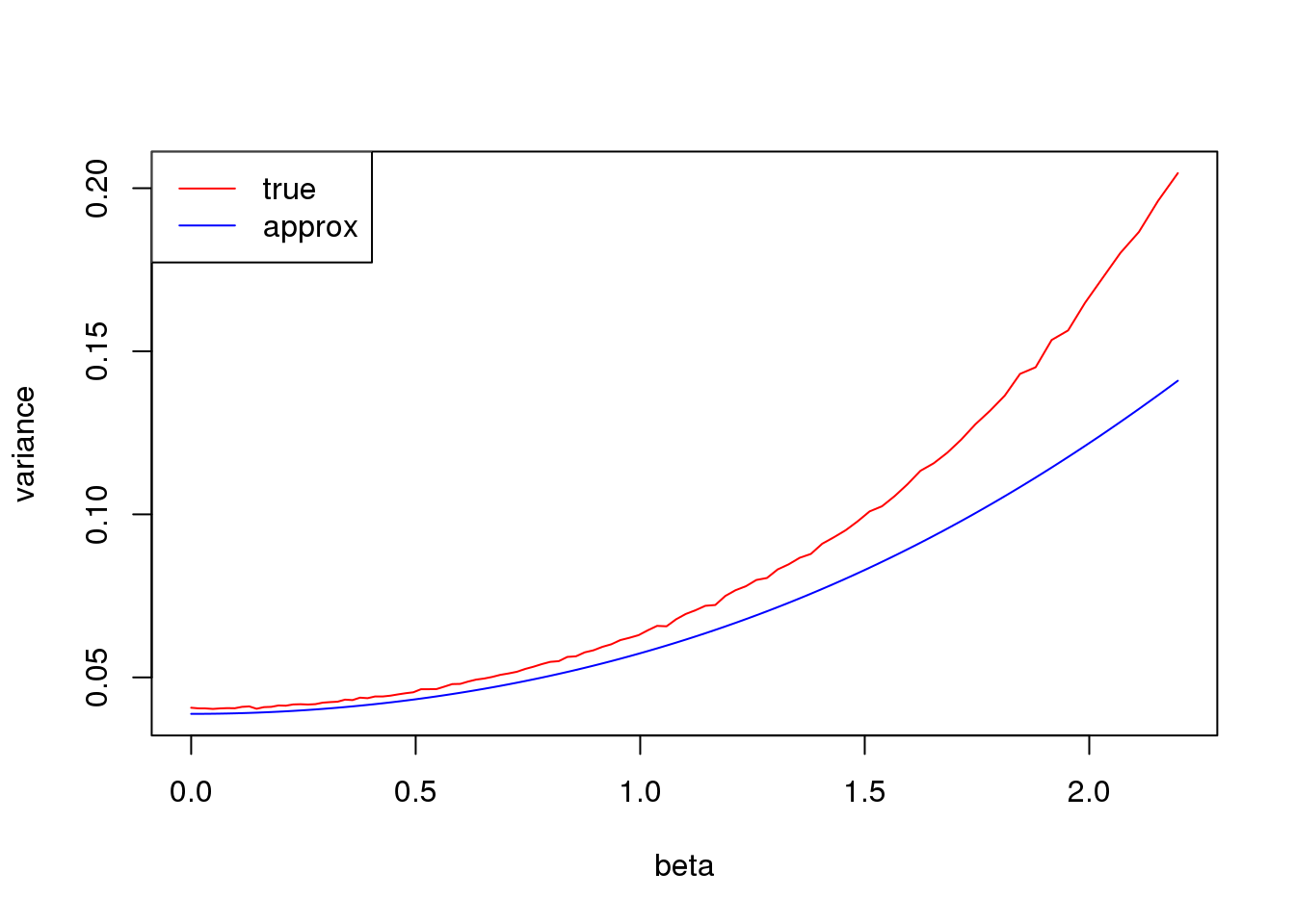
| Version | Author | Date |
|---|---|---|
| 7177fb2 | DongyueXie | 2020-04-01 |
Small \(np\)
set.seed(12345)
p_list = seq(0.1,0.5,length.out = 100)

n = 5
s = 0.5


true_var = c()
approx_var = c()

for(p in p_list){
  y1 = rbinom(1e5,n,p)
  y2 = rbinom(1e5,n,1-p)
  true_var = c(true_var,var(log(y1+s))+var(log(y2+s)))
  approx_var = c(approx_var,var_log(n,p,s)+var_log(n,1-p,s))
}

par(mfrow=c(1,1))

plot(log(1/p_list-1),true_var,xlab = 'beta', ylab= 'variance',type='l',col=2,ylim = range(c(true_var,approx_var)))
lines(log(1/p_list-1),approx_var,col=4)
legend('topright',c('true','approx'),lty=c(1,1),col=c(2,4))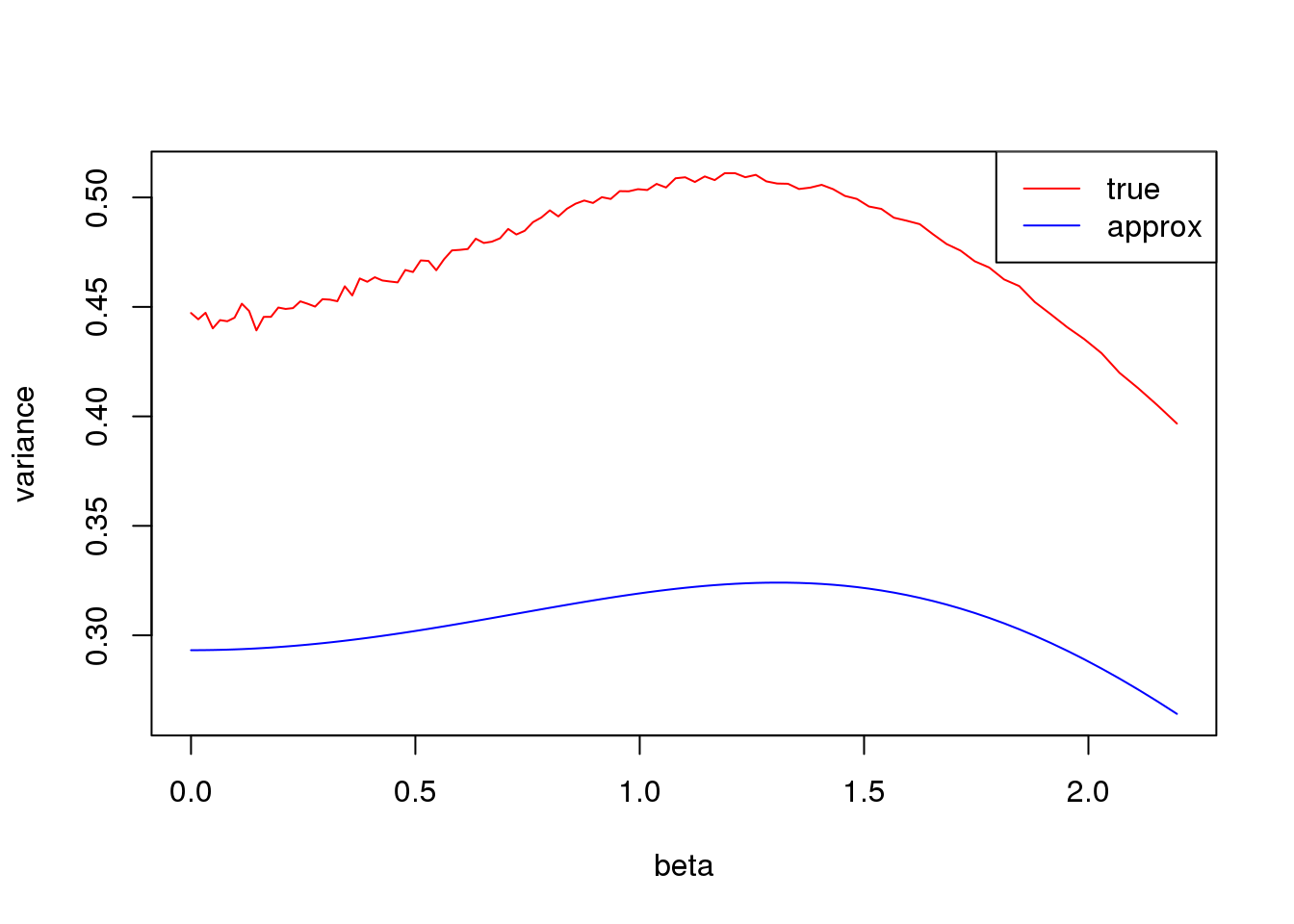
| Version | Author | Date |
|---|---|---|
| 7177fb2 | DongyueXie | 2020-04-01 |
set.seed(12345)
n_list = 0:100


s = 0.5
p = 0.1

true_var = c()
approx_var = c()

for(n in n_list){
  y1 = rbinom(1e5,n,p)
  y2 = rbinom(1e5,n,1-p)
  true_var = c(true_var,var(log(y1+s))+var(log(y2+s)))
  approx_var = c(approx_var,var_log(n,p,s)+var_log(n,1-p,s))
}

plot(n_list,true_var,xlab = 'n', ylab= 'variance',type='l',col=2)
lines(n_list,approx_var,col=4)
legend('topleft',c('true','approx'),lty=c(1,1),col=c(2,4))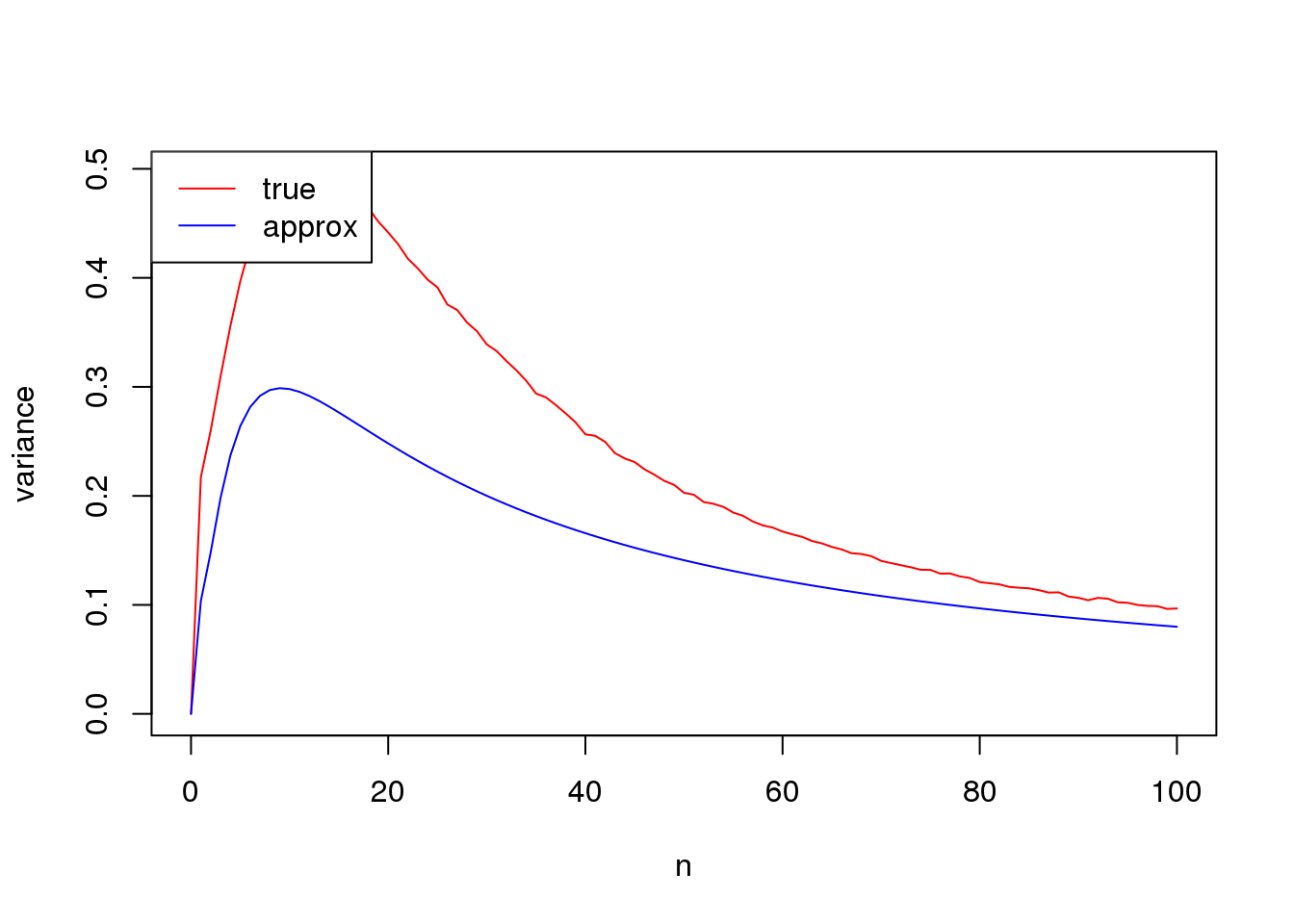
| Version | Author | Date |
|---|---|---|
| 7177fb2 | DongyueXie | 2020-04-01 |
Let’s start with the simplest case: we have a count matrix \(Y\), whose all entries are the same! Then we apply binomial thinning to \(Y\).
In the following simulation, we set the number of samples to be \(n=500\), the number of genes \(p=5000\) and entries of \(Y\) vary from \(100, 50, 30, 20, 10, 5, 1.\) Half of samples are from group 1 and the rest are from group 2. About \(90\%\) of genes have no effects and the rest have effects \(\beta_j\) generated from standard normal distribution.
We fit a simple linear regression to each gene with log transformed counts and compare the log-likelihood from ash, setting \(\alpha=0\) and \(\alpha=1\), and plot \(\beta\) vs \(\hat\beta\) as well as \(\beta\) vs \(s.e.(\hat\beta)\) for each case.
#'@param Z count matrix, sample by features
#'@param x 1 for group 1, 0 for group 2
#'@param beta effect of fearures,  0 for null.
#'@return W, thinned matrix
bi_thin = function(Z,x,beta){

  n=nrow(Z)
  p=ncol(Z)

  # group index
  g1 = which(x==1)
  g2 = which(x==0)


  p2 = 1/(1+exp(beta))
  p1 = 1-p2
  P = matrix(nrow = n,ncol = p)
  P[g1,] = t(replicate(length(g1),p1))
  P[g2,] = t(replicate(length(g2),p2))

  W = matrix(rbinom(n*p,Z,P),nrow=n)

  W
}

library(limma)

n=500
p=5000
set.seed(12345)

loglik0 = c()
auc0 = c()
loglik1 = c()
auc1 = c()

par(mfrow = c(1,2))
for(ni in c(100,50,30,20,10,5,1)){
  Y = matrix(rep(ni,n*p),nrow=p,ncol=n)

  group_idx = c(rep(1,n/2),rep(0,n/2))
  X = model.matrix(~group_idx)

  b = seq(1,10,length.out = p)
  b[sample(1:p,0.9*p)] = 0
  which_null = 1*(b==0)

  W = bi_thin(t(Y),group_idx,b)

  lmout <- limma::lmFit(object = t(log(W+0.5)), design = X)

  ash0 = ashr::ash(lmout$coefficients[, 2],lmout$stdev.unscaled[, 2]*lmout$sigma,alpha=0)
  loglik0 = c(loglik0,ash0$loglik)
  auc0 = c(auc0,pROC::roc(which_null,ash0$result$lfsr)$auc)

  ash1 = ashr::ash(lmout$coefficients[, 2],lmout$stdev.unscaled[, 2]*lmout$sigma,alpha=1)
  loglik1 = c(loglik1,ash1$loglik)
  auc1 = c(auc1,pROC::roc(which_null,ash1$result$lfsr)$auc)


  plot((b),lmout$coefficients[, 2],xlab='beta',ylab='estimated',col='grey60',main=paste('count:',ni))
  abline(a=0,b=1)
  plot(abs(b),lmout$stdev.unscaled[, 2]*lmout$sigma,xlab='absolute value of beta',ylab='sd of beta_hat',main=paste('count:',ni))
}

knitr::kable(cbind(c(100,50,30,20,10,5,1),loglik0,loglik1),col.names = c('Y','alpha0','alpha1'),
             caption = 'log likelihood')

knitr::kable(cbind(c(100,50,30,20,10,5,1),auc0,auc1),col.names = c('Y','alpha0','alpha1'),
             caption = 'AUC')
So when counts in \(Y\) are large, setting \(\alpha=1\) gives higher likelihood. Estimated \(\beta\)s are close to true \(\beta\)s and apparently, scale of \(\beta\) and \(var(\hat\beta)\) are positively correlated. While when counts in \(Y\) are small, things are opposite.
sessionInfo()R version 3.5.1 (2018-07-02)
Platform: x86_64-pc-linux-gnu (64-bit)
Running under: Scientific Linux 7.4 (Nitrogen)
Matrix products: default
BLAS/LAPACK: /software/openblas-0.2.19-el7-x86_64/lib/libopenblas_haswellp-r0.2.19.so
locale:
[1] LC_CTYPE=en_US.UTF-8 LC_NUMERIC=C
[3] LC_TIME=en_US.UTF-8 LC_COLLATE=en_US.UTF-8
[5] LC_MONETARY=en_US.UTF-8 LC_MESSAGES=en_US.UTF-8
[7] LC_PAPER=en_US.UTF-8 LC_NAME=C
[9] LC_ADDRESS=C LC_TELEPHONE=C
[11] LC_MEASUREMENT=en_US.UTF-8 LC_IDENTIFICATION=C
attached base packages:
[1] parallel stats graphics grDevices utils datasets methods
[8] base
other attached packages:
[1] Matrix_1.2-15 Biobase_2.42.0 BiocGenerics_0.28.0
loaded via a namespace (and not attached):
[1] Rcpp_1.0.2 pillar_1.3.1 plyr_1.8.4
[4] compiler_3.5.1 later_0.7.5 git2r_0.26.1
[7] workflowr_1.6.0 iterators_1.0.10 tools_3.5.1
[10] digest_0.6.18 tibble_2.1.1 gtable_0.2.0
[13] evaluate_0.12 lattice_0.20-38 pkgconfig_2.0.2
[16] rlang_0.4.0 foreach_1.4.4 yaml_2.2.0
[19] dplyr_0.8.0.1 stringr_1.3.1 knitr_1.20
[22] pROC_1.13.0 fs_1.3.1 tidyselect_0.2.5
[25] rprojroot_1.3-2 grid_3.5.1 glue_1.3.0
[28] R6_2.3.0 rmarkdown_1.10 mixsqp_0.2-2
[31] limma_3.38.2 purrr_0.3.2 ggplot2_3.1.1
[34] ashr_2.2-39 magrittr_1.5 whisker_0.3-2
[37] scales_1.0.0 backports_1.1.2 promises_1.0.1
[40] codetools_0.2-15 htmltools_0.3.6 MASS_7.3-51.1
[43] assertthat_0.2.0 colorspace_1.3-2 httpuv_1.4.5
[46] stringi_1.2.4 lazyeval_0.2.1 munsell_0.5.0
[49] doParallel_1.0.14 pscl_1.5.2 truncnorm_1.0-8
[52] SQUAREM_2017.10-1 crayon_1.3.4