workflowr

• Summary
• Checks
• Past versions

Last updated: 2025-04-28

Checks: 7 0

Knit directory: DigitalResearchSkillsNetwork/

This reproducible R Markdown analysis was created with workflowr (version 1.7.1). The Checks tab describes the reproducibility checks that were applied when the results were created. The Past versions tab lists the development history.

---

R Markdown file: up-to-date

Great! Since the R Markdown file has been committed to the Git repository, you know the exact version of the code that produced these results.

Environment: empty

Great job! The global environment was empty. Objects defined in the global environment can affect the analysis in your R Markdown file in unknown ways. For reproduciblity it’s best to always run the code in an empty environment.

Seed: set.seed(1337)

The command set.seed(1337) was run prior to running the code in the R Markdown file. Setting a seed ensures that any results that rely on randomness, e.g. subsampling or permutations, are reproducible.

Session information: recorded

Great job! Recording the operating system, R version, and package versions is critical for reproducibility.

Cache: none

Nice! There were no cached chunks for this analysis, so you can be confident that you successfully produced the results during this run.

File paths: relative

Great job! Using relative paths to the files within your workflowr project makes it easier to run your code on other machines.

Repository version: f620219

Great! You are using Git for version control. Tracking code development and connecting the code version to the results is critical for reproducibility.

The results in this page were generated with repository version f620219. See the Past versions tab to see a history of the changes made to the R Markdown and HTML files.

Note that you need to be careful to ensure that all relevant files for the analysis have been committed to Git prior to generating the results (you can use wflow_publish or wflow_git_commit). workflowr only checks the R Markdown file, but you know if there are other scripts or data files that it depends on. Below is the status of the Git repository when the results were generated:

Ignored files:
    Ignored:    .DS_Store
    Ignored:    .Rhistory
    Ignored:    analysis/.DS_Store
    Ignored:    analysis/.RData
    Ignored:    analysis/.Rhistory
    Ignored:    analysis/adit/.DS_Store

Unstaged changes:
    Modified:   analysis/202504.Rmd

Note that any generated files, e.g. HTML, png, CSS, etc., are not included in this status report because it is ok for generated content to have uncommitted changes.

---

These are the previous versions of the repository in which changes were made to the R Markdown (analysis/202504_Workshop.Rmd) and HTML (docs/202504_Workshop.html) files. If you’ve configured a remote Git repository (see ?wflow_git_remote), click on the hyperlinks in the table below to view the files as they were in that past version.

File	Version	Author	Date	Message
Rmd	f620219	DrThomasOneil	2025-04-28	wflow_publish("analysis/202504_Workshop.Rmd")
html	94e37b3	DrThomasOneil	2025-04-28	Build site.
Rmd	ab18949	DrThomasOneil	2025-04-28	wflow_publish("analysis/202504_Workshop.Rmd")
html	2c16dc0	DrThomasOneil	2025-04-28	Build site.
Rmd	0925bfe	DrThomasOneil	2025-04-28	wflow_publish("analysis/202504_Workshop.Rmd")
html	ec75f7d	DrThomasOneil	2025-04-26	Build site.
Rmd	e8a3722	DrThomasOneil	2025-04-26	wflow_publish("analysis/202504_Workshop.Rmd")
html	938818e	DrThomasOneil	2025-04-14	Build site.
html	ed690e6	DrThomasOneil	2025-04-14	Build site.
Rmd	1e8103e	DrThomasOneil	2025-04-14	wflow_publish("analysis/*.Rmd")
html	cb886ef	DrThomasOneil	2025-04-10	Build site.
Rmd	eb0a784	GitHub	2025-04-09	Update 202504_Workshop.Rmd
html	f6c0433	YuchenLi	2025-04-09	Build site.
Rmd	04953d6	YuchenLi	2025-04-09	wflow_publish("analysis/*.Rmd")
html	8d78b0f	YuchenLi	2025-04-09	Build site.
html	7421f69	DrThomasOneil	2025-04-08	Build site.
html	f2d3385	DrThomasOneil	2025-03-24	update
html	517dcf9	DrThomasOneil	2025-03-24	Build site.
html	6a4432b	DrThomasOneil	2025-03-24	Build site.
html	1f218f3	DrThomasOneil	2025-03-24	Build site.
html	dca90e9	DrThomasOneil	2025-03-24	Build site.
html	1d1c076	DrThomasOneil	2025-03-24	Build site.
html	956ba9b	DrThomasOneil	2025-03-24	Build site.
Rmd	6b72e34	DrThomasOneil	2025-03-24	wflow_publish(c("analysis/*.Rmd"))
html	d600337	DrThomasOneil	2025-03-18	Build site.
html	b537f69	DrThomasOneil	2025-03-18	Build site.
html	b7982e9	DrThomasOneil	2025-03-16	Build site.
html	fc5dd81	DrThomasOneil	2025-03-16	Build site.
html	8e1c1a3	DrThomasOneil	2025-03-16	Build site.
Rmd	d75e5ae	DrThomasOneil	2025-03-16	wflow_publish(c("analysis/*.Rmd"))

---

Flow Cytometry in R: A Hands-On Introduction

This beginner-friendly, hands-on workshop will guide users through a complete flow cytometry analysis workflow in R, from loading data to visualizing results. Through practical exercises, we’ll cover essential steps like generating histograms and scatterplots, extracting summary statistics, subsetting data, and performing dimension reduction and clustering—all while demonstrating the advantages of reproducible reports with RMarkdown.

Whether you’re new to R or just curious about coding your analyses, this session will show you how accessible and powerful R can be for flow cytometry.

Your Demonstrators:

• Thomas O’Neil
  
• Yuchen Li (Online)

Author: Yuchen Li, Thomas O’Neil

Zoom link (recorded)

Introduction

In this workshop, we aim to give an overview of what is possible for flow analysis in R. We will touch on two workflows:

• data visualisation and data collection

• dimension reduction and clustering

We’ll use a 25-colour flow cytometry dataset of innate lymphoid cells (ILC), natural killer cells (NK), and innate-like T cells in human intestinal tissues, after excluding dead cells, doublets, mast cells and basophils, hematopoietic stem cells, myeloid cells and granulocytes, and B cells.

The original data was published as is available in OMIP-082

Before going further:

• Dont forget to provide any feedback by emailing us at drsn@wimr.org.au or filling out the feedback form

• Vote on the next workshop!

Setup

We’ll take you through steps from the beginning, installing packages and loading data.

Preparation: packages and directories

Packages are collections of functions. Many are not in-built in the base R but they do pretty cool things, enabling generating pretty plots, performing data wrangling in an efficient way, etc. R also has a large developer community, with many community-developed packages available on platforms like Bioconductor or GitHub.

# Install packages used in this workshop.

#install.packages("tidyverse")
#install.packages("ggridges")
#install.packages("GGally")
#install.packages("cowplot")
#install.packages("data.table")
#install.packages("BiocManager")

#BiocManager::install("FuseSOM")
#BiocManager::install("FlowSOM")

#if(!require('remotes')) {install.packages('remotes')}
#remotes::install_github(repo = "immunedynamics/spectre")


# Load packages
library(tidyverse)
library(ggridges)
library(cowplot)
library(Spectre)
library(FuseSOM)
library(FlowSOM)
library(GGally)
library(umap)
library(Rtsne)
library(data.table)

theme_set(theme_classic())

Create some folders for plots and data.

dir.create("plots")
dir.create("data")
download.file("https://raw.githubusercontent.com/DrThomasOneil/Digital-Research-Skills-Network/refs/heads/main/docs/assets/downloads/example_flowdata_omip082_20k.csv", destfile = "data/example_flowdata_omip082_20k.csv")
# Add `method = "curl"` in the download.file() if you are a Windows user and this line didn't work for you.

Setting seed is crucial for reproducibility:

It’s a number of your choice, which pins down the “way” that how the random process will be performed when you re-run these codes. (Easier example: Say if you randomly take 10 numbers with a mean of 50, there will be tonnes of ways to generate the numbers. But a seed ensures that the report always returns the same set of numbers. It’s the similar idea when you run other algorithms including randomness, e.g. clustering and generating a UMAP).

set.seed(1337)

Load flow cytometry data

The expression data is stored in a .csv file. We’ll first load this in.

# Read the .csv file in the working directory.
ILC <- read.csv("data/example_flowdata_omip082_20k.csv")

Have a look at the broad features of this dataset. In this dataset, the channel names are stored as column names. Each row represents a cell, storing expression values in each channel.

# Dimension: number of cells x number of channels.
dim(ILC)

# Check the column names.
colnames(ILC)

The column names are wordy, with markers, fluorophores, and channels. We just need the marker names to proceed. The first column ‘X’ is just indexing the number of rows. It’s not necessary either.

Remove the first column.

# This keeps the 2-33 columns in the dataset, and store the change.
ILC <- ILC[, -1]
colnames(ILC)

 [1] "FSC.A"                        "FSC.H"                       
 [3] "FSC.W"                        "SSC.A"                       
 [5] "SSC.H"                        "SSC.W"                       
 [7] "NKp44_BB515.B515_30.A"        "Lineage_PerCP.Cy55.B710_50.A"
 [9] "CD45_BB790.B820_60.A"         "CD103_APC.R670_30.A"         
[11] "FVS_700.R710_40.A"            "CD4_APC_Cy7.R820_60.A"       
[13] "HLA.DR_BUV395.U379_28.A"      "CD16_BUV496.U515_30.A"       
[15] "CD3_BUV563.U586_15.A"         "CD94_BUV615.U610_20.A"       
[17] "CD39_BUV661.U670_30.A"        "CD56_BUV737.U740_35.A"       
[19] "TCRVA72_BUV805.U820_60.A"     "CKIT_BV421.V427_25.A"        
[21] "CD14_CD19_BV480.V474_25.A"    "CD49D_BV510.V525_50.A"       
[23] "CD244_SB600.V610_20.A"        "CD161_B650.V677_20.A"        
[25] "TCRgt_BV711.V710_50.A"        "CD69_BV750.V750_30.A"        
[27] "CD25_BV786.V820_60.A"         "ITAGB7_PE.Y586_15.A"         
[29] "CRTH2_PEDAZZLE594.Y610_20.A"  "NKp46_PECy5.Y670_30.A"       
[31] "CD127_PECy7.Y820_60.A"        "Time"                        

# Same with it, you can just enter the column indexes from 2-33.
# ILC <-ILC[,c(2:33)]

Change the column names.

# Substitute everything after the first '_' with an empty "" in the column names that have the pattern "_" and something.
colnames(ILC) <- sub("_.*","",colnames(ILC)) #'_' is the exact character in the names, the '.' means 'any character', '*' means 'any of the preceding things'. 

colnames(ILC)

 [1] "FSC.A"   "FSC.H"   "FSC.W"   "SSC.A"   "SSC.H"   "SSC.W"   "NKp44"  
 [8] "Lineage" "CD45"    "CD103"   "FVS"     "CD4"     "HLA.DR"  "CD16"   
[15] "CD3"     "CD94"    "CD39"    "CD56"    "TCRVA72" "CKIT"    "CD14"   
[22] "CD49D"   "CD244"   "CD161"   "TCRgt"   "CD69"    "CD25"    "ITAGB7" 
[29] "CRTH2"   "NKp46"   "CD127"   "Time"   

Fix up the broken names FVS700 and CD14&CD19.

# This tells R to: find which of the column equals "FVS" among all columns in the data, then change it to FVS700.
colnames(ILC)[colnames(ILC) == "FVS"] <- "FVS700"
colnames(ILC)[colnames(ILC) == "CD14"] <- "CD14.CD19"

# Have a look
colnames(ILC)

 [1] "FSC.A"     "FSC.H"     "FSC.W"     "SSC.A"     "SSC.H"     "SSC.W"    
 [7] "NKp44"     "Lineage"   "CD45"      "CD103"     "FVS700"    "CD4"      
[13] "HLA.DR"    "CD16"      "CD3"       "CD94"      "CD39"      "CD56"     
[19] "TCRVA72"   "CKIT"      "CD14.CD19" "CD49D"     "CD244"     "CD161"    
[25] "TCRgt"     "CD69"      "CD25"      "ITAGB7"    "CRTH2"     "NKp46"    
[31] "CD127"     "Time"     

Time gate QC.

The data is already preprocessed in FlowJo. But if you are interested, you can view the Time gate, and filter the data based on this in R.

ggplot(ILC, aes(x = Time, y = FSC.A))+
  geom_bin_2d(bins = 200, show.legend = FALSE)+
    scale_fill_gradientn(colours = c("blue", "green", "yellow", "red"))+
  geom_vline(xintercept = 4600000)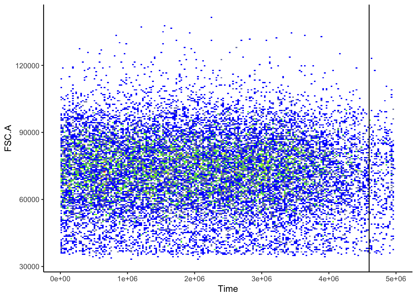

Past versions of unnamed-chunk-9-1.png

Version	Author	Date
2c16dc0	DrThomasOneil	2025-04-28
ec75f7d	DrThomasOneil	2025-04-26

# Filter out the cells above the threshold.
ILC <- ILC[ILC$Time < 4600000,]
ggplot(ILC, aes(x = Time, y = FSC.A))+
  geom_bin_2d(bins = 200, show.legend = FALSE)+
    scale_fill_gradientn(colours = c("blue", "green", "yellow", "red"))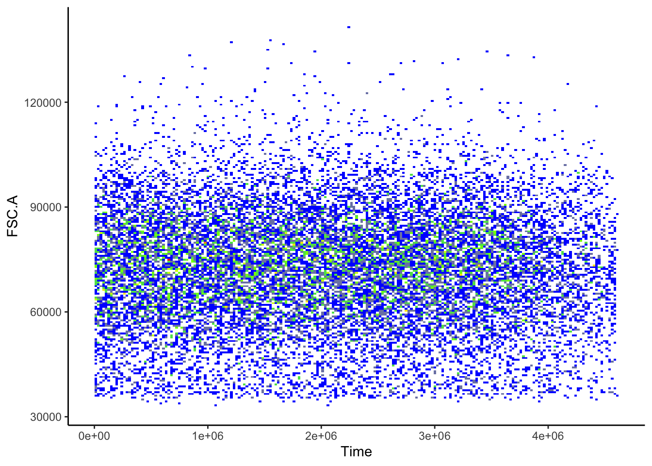

Past versions of unnamed-chunk-9-2.png

Version	Author	Date
2c16dc0	DrThomasOneil	2025-04-28

Visualisations

Transformations

Raw Flow Cytometry data looks bad!

ILC %>% ggplot(aes(x=CD4, y=CD3))+        
  geom_point()

Past versions of unnamed-chunk-10-1.png

Version	Author	Date
2c16dc0	DrThomasOneil	2025-04-28
ec75f7d	DrThomasOneil	2025-04-26

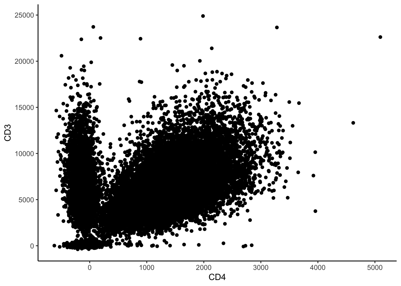
So we transform the data to make it look better. In FlowJo, when you adjust the axes, you can see several transformations available. One is arcsinh (the inverse of hyperbolic sin, if you want to get mathy). Smaller values centre around zero, and larger values separate, giving the appearance that we’re familiar with.

We are also able to adjust the level of transformation by dividing the values by some cofactor.

# decide on a cofactor - try changing it and seeing how the data changes
cofactor = 500
ILC_transf <- asinh(ILC[,7:31]/cofactor) #7:31 are the columns with markers.

ILC_transf <- cbind(ILC_transf, ILC[,c(1:6,32)]) # Add the first 6 columns & time back in.

ILC_transf %>% ggplot(aes(x=CD4, y=CD3))+
  geom_bin_2d(bins = 200, show.legend=T)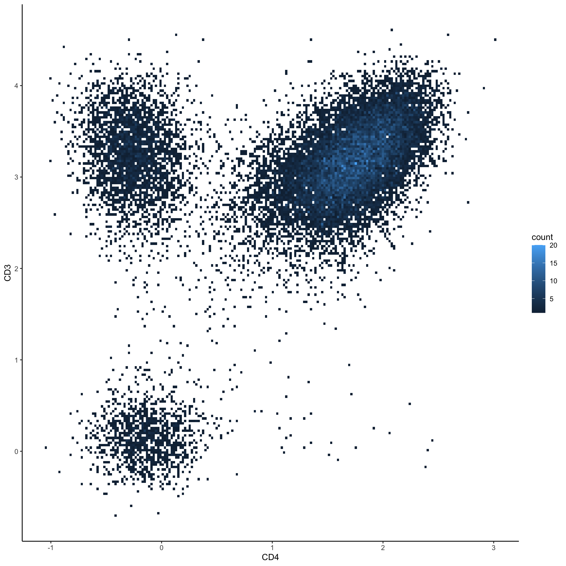

Past versions of unnamed-chunk-11-1.png

Version	Author	Date
2c16dc0	DrThomasOneil	2025-04-28
ec75f7d	DrThomasOneil	2025-04-26

You can view it for all markers together.

# Initialize an empty list to store the plots
plots <- list()
# Define the x-axis marker for the plots
xaxis = "CD39" # Choose an x-axis marker for comparison

# Loop through each column in the dataset
for(i in 1:ncol(ILC_transf)) {
  # Get the marker name for the current column
  Marker <- colnames(ILC_transf)[i]
  
  # Generate a 2D bin plot for the current marker against the chosen x-axis marker
  p <- ILC_transf %>% 
        ggplot(aes_string(x = xaxis, y = Marker)) +        
        geom_bin_2d(bins = 200, show.legend = FALSE) + # Create a heatmap-style scatter plot
        scale_fill_gradientn(colors = c("blue", "yellow", "red")) # Define the color gradient
  
  # Add the generated plot to the list
  plots[[i]] <- p
}

# Combine all the plots into a grid layout and display them
cowplot::plot_grid(plotlist = plots)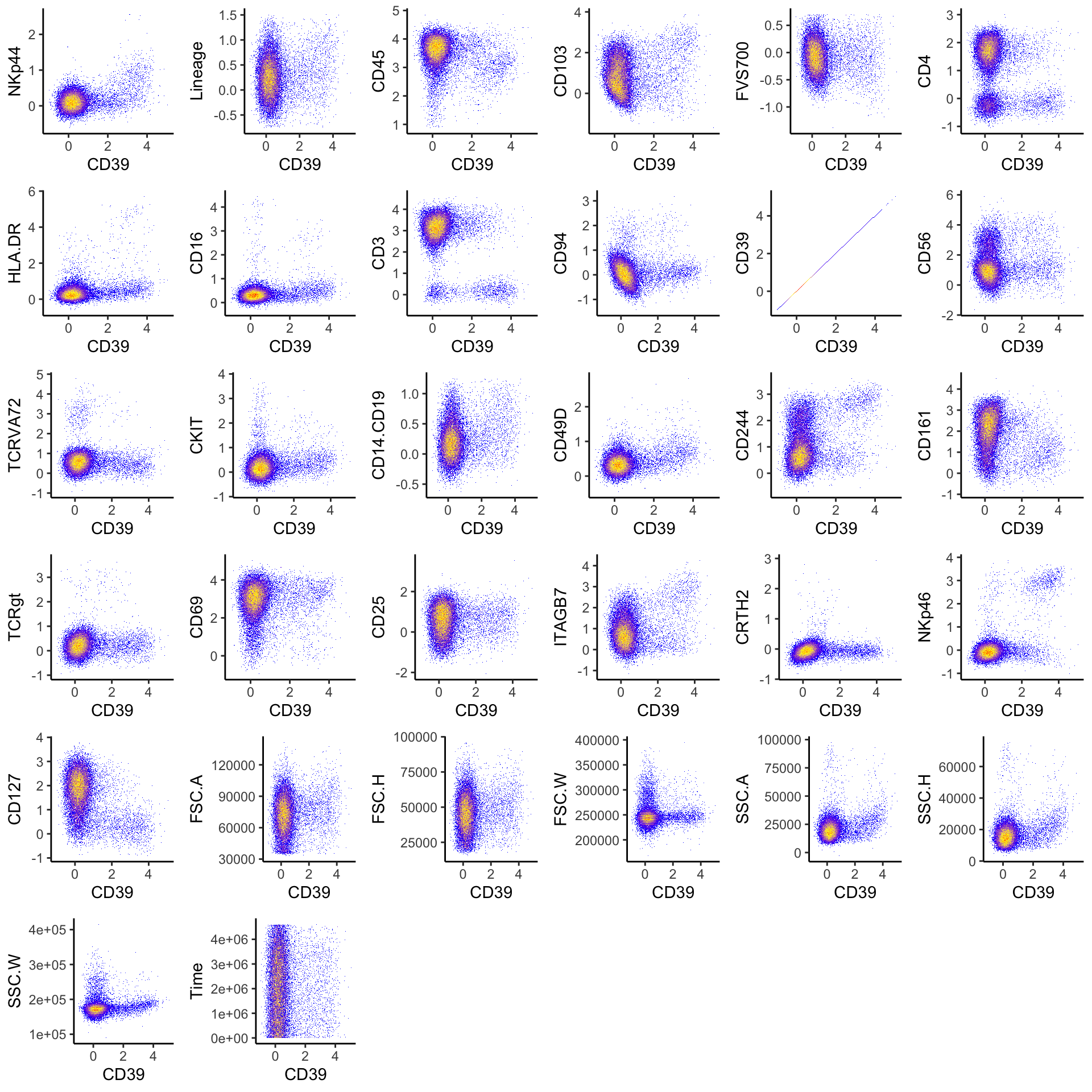

Past versions of unnamed-chunk-12-1.png

Version	Author	Date
2c16dc0	DrThomasOneil	2025-04-28

rm(plots)

This code demonstrates how you would manually transform individual columns in the dataset using different cofactors for each marker. It creates a new dataset (ILC_transf_indiv) where specific columns are transformed using the asinh function with their respective cofactors. This allows for more granular control over transformations.

ILC_transf_indiv <- ILC
ILC_transf_indiv[, "CD3"] <- asinh(ILC[,"CD3"]/1000)
ILC_transf_indiv[, "CD4"] <- asinh(ILC[,"CD4"]/500)
# and so on...

# Visualize it
ILC_transf_indiv %>% ggplot(aes(x=CD3, y=CD4))+        
        geom_bin_2d(bins = 200, show.legend=F) +
        scale_fill_gradientn(colors = c("blue",  "yellow", "red"))

rm(ILC_transf_indiv)

Histograms

We can visualize the marker expressions via histograms and density plots.

# For example, this generates a histogram of CD3 expression.
ILC_transf %>%
  ggplot(aes(x = CD3))+
  # Plot the histogram, and change the fill colour to lightblue, the line colour to black.
  geom_histogram(bins = 35, fill = "lightblue", colour ="black")+
  # Add labels
  ylab("Frequency")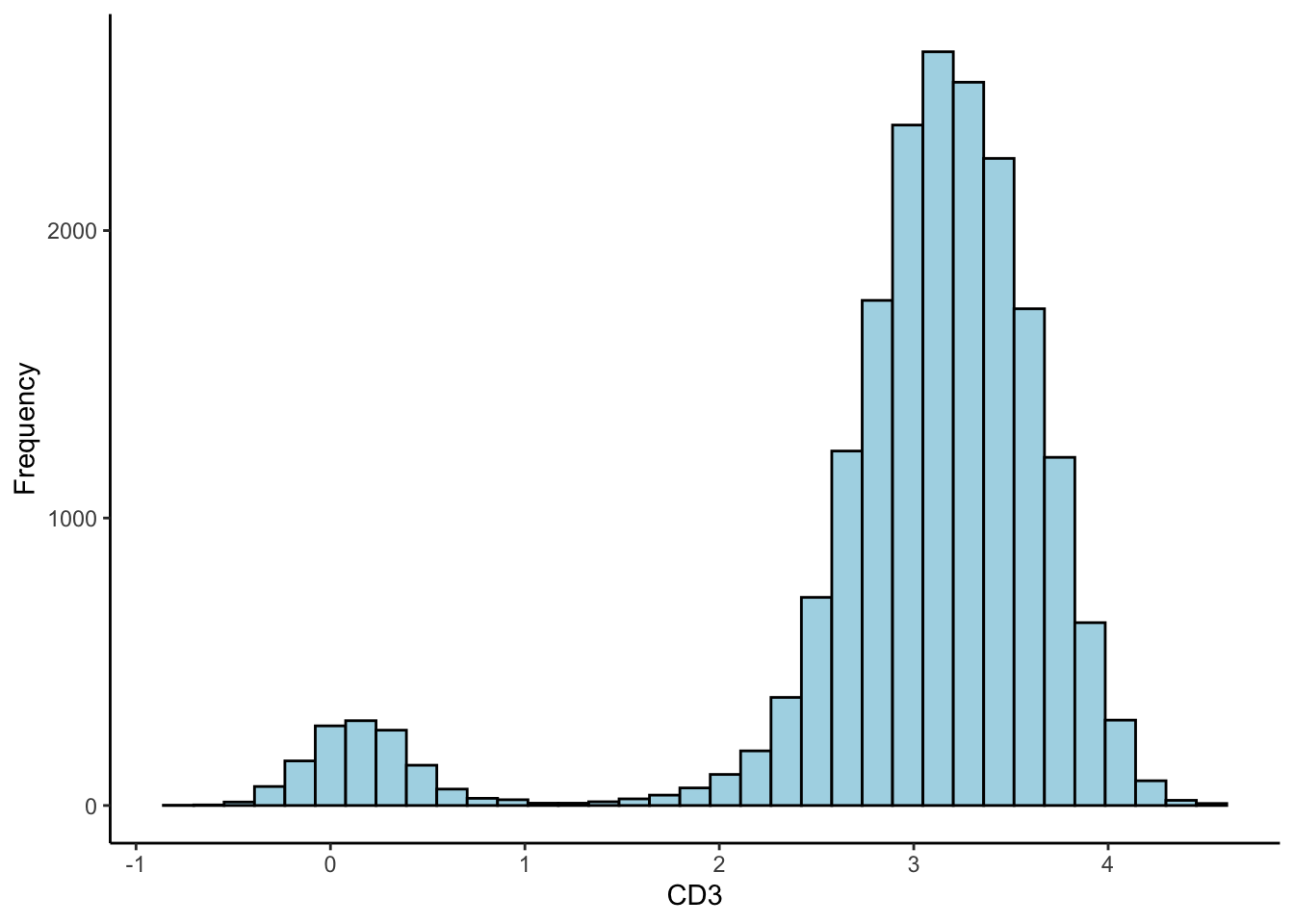

Past versions of unnamed-chunk-14-1.png

Version	Author	Date
2c16dc0	DrThomasOneil	2025-04-28
ec75f7d	DrThomasOneil	2025-04-26

# A density plot.
ILC_transf %>%
  ggplot(aes(x = CD3))+
  geom_density(linewidth = 0.7, colour = "red4", aes(fill = "red"), alpha = 0.5,show.legend = FALSE)+
  ylab("Density")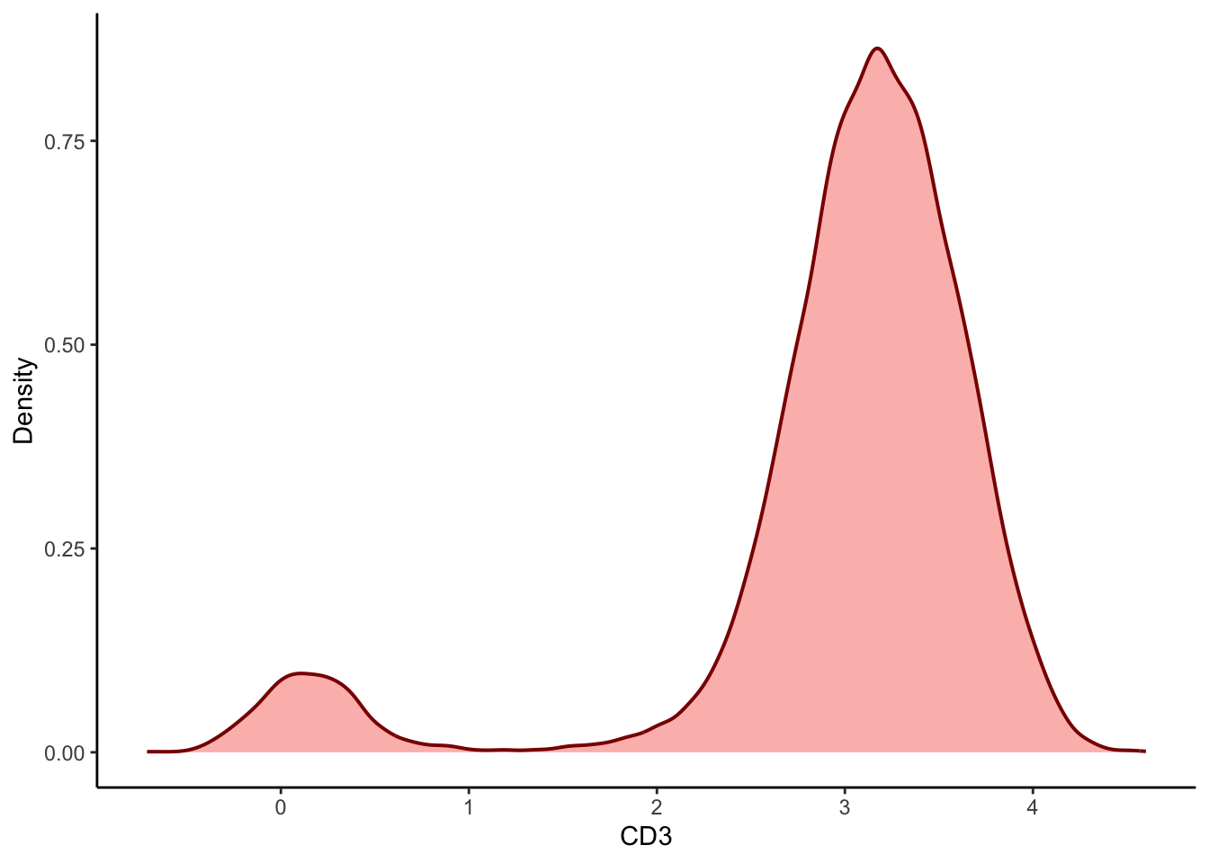

Past versions of unnamed-chunk-14-2.png

Version	Author	Date
2c16dc0	DrThomasOneil	2025-04-28

We can loop through the channels and create a density plot for all 25 markers.

# Initialise an empty list to store the plots
plots<- list()

# Loop through each column in the dataset
for (i in 1:ncol(ILC_transf)){

  # Get the marker name for the current column
  Marker <- colnames(ILC_transf)[i]

  # Generate the histogram for the current marker
  p <- ILC_transf %>%
  ggplot(aes(x = .data[[Marker]]))+
    geom_density(linewidth = 0.7, colour = "red4", aes(fill = "red"), alpha = 0.5,show.legend = FALSE)+
    labs(x=Marker,y="")+
    theme(axis.text = element_text(size=1))

  # Add the generated plot to the list
  plots[[i]] <- p
}

plot_grid(plotlist = plots[1:25])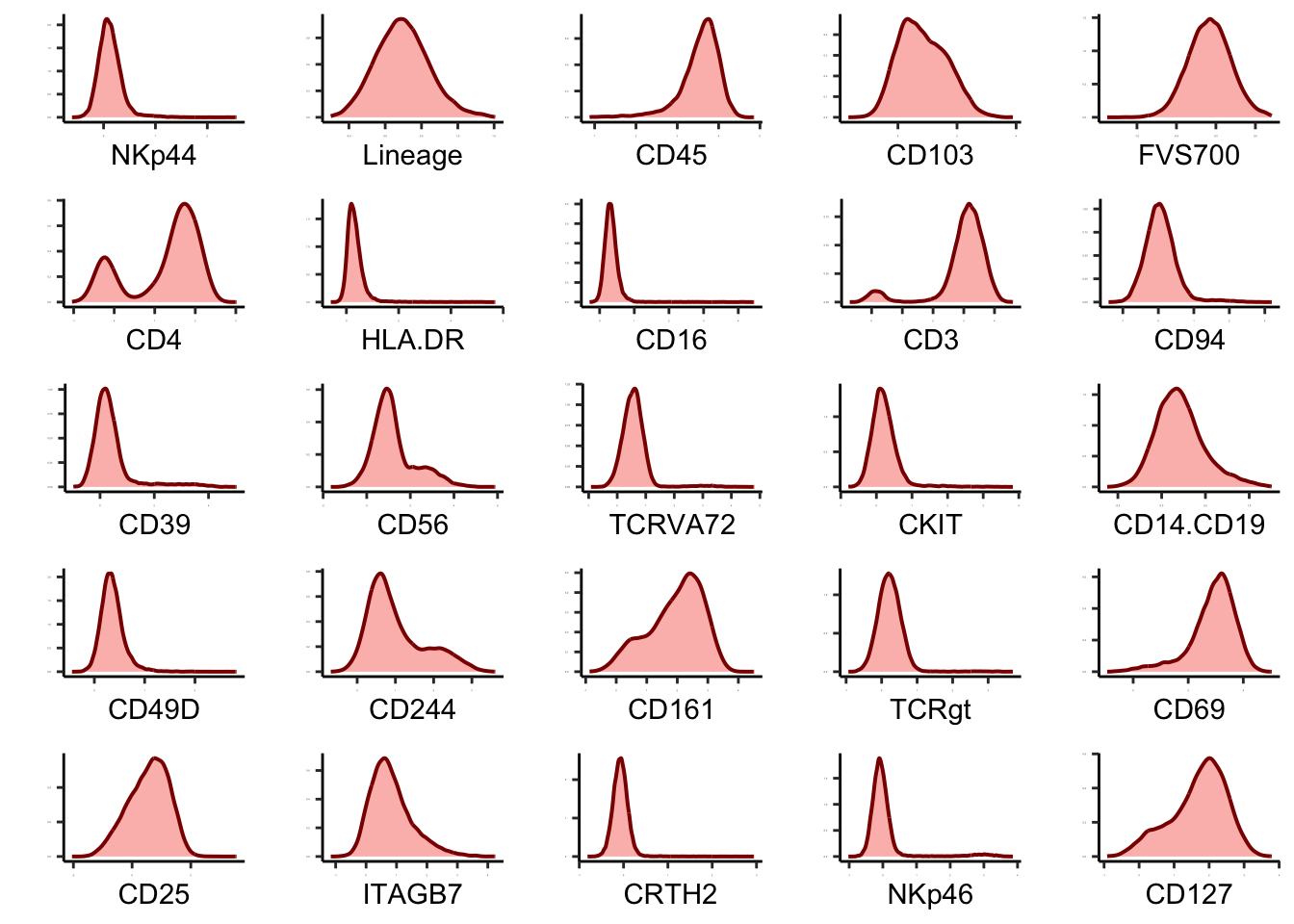

Past versions of unnamed-chunk-15-1.png

Version	Author	Date
2c16dc0	DrThomasOneil	2025-04-28
ec75f7d	DrThomasOneil	2025-04-26

rm(plots)

Scatter plot

Like what we do in Flowjo, we can visualize 2 markers’ expressions, We can generate scatterplots.

ILC_transf %>%
  ggplot(aes(x = CD4, y = CD3))+
  geom_point(color="blue", alpha=0.1)

Past versions of unnamed-chunk-16-1.png

Version	Author	Date
2c16dc0	DrThomasOneil	2025-04-28
ec75f7d	DrThomasOneil	2025-04-26

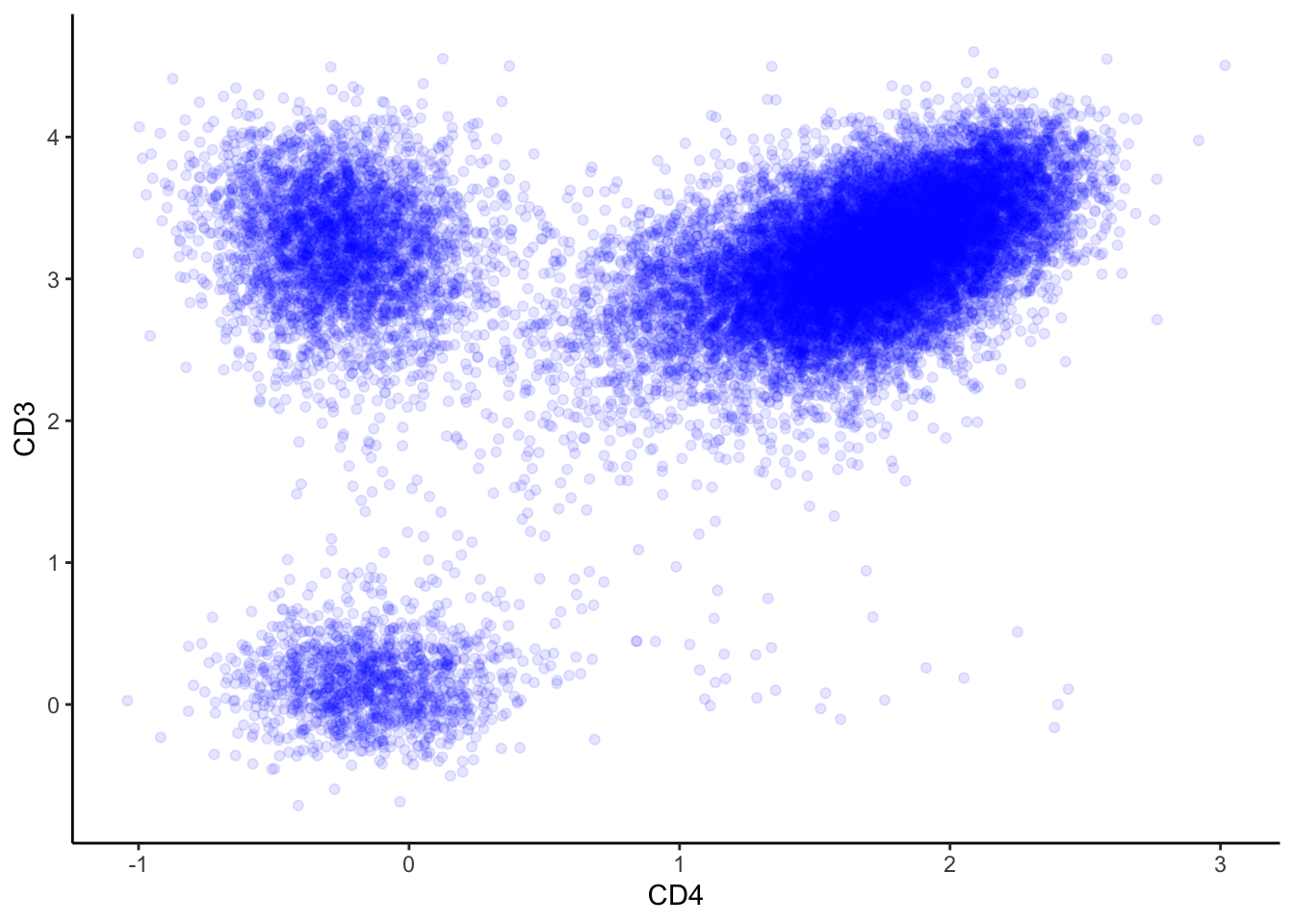
# Generate a scatterplot with a density overlay.
ILC_transf %>% ggplot(aes(x=CD4, y=CD3))+        
  geom_bin_2d(bins = 200, show.legend = F)+
  scale_fill_gradientn(colors = c("blue",  "yellow", "red"))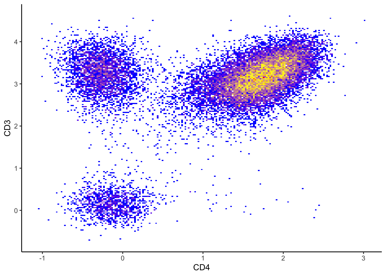

Past versions of unnamed-chunk-16-2.png

Version	Author	Date
2c16dc0	DrThomasOneil	2025-04-28
ec75f7d	DrThomasOneil	2025-04-26

Contour plot

And a 2-marker countour plot. You can easily make it more stylish by adding layers in ggplot!

# A contour plot of CD3 and CD4 expression values.
ILC_transf %>%
  ggplot(aes(x = CD3, y = CD4))+
  geom_density_2d(colour = "black", bins=50)+
  xlab("CD3 BUV563")+
  ylab("CD4 APC-Cy7")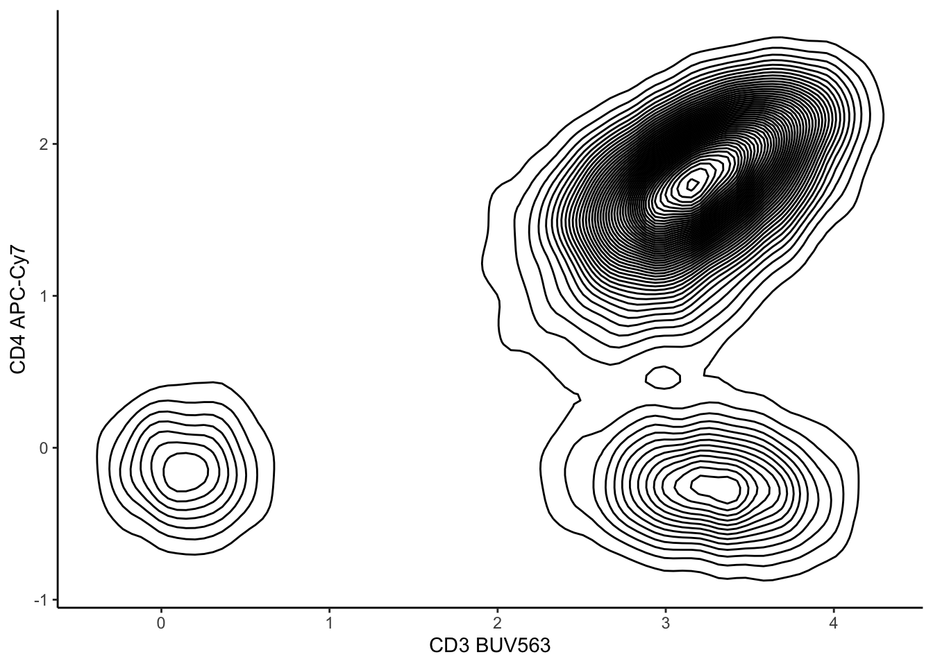

Past versions of unnamed-chunk-17-1.png

Version	Author	Date
2c16dc0	DrThomasOneil	2025-04-28
ec75f7d	DrThomasOneil	2025-04-26

# A contour plot of CD3 and CD4 expression over a scatter plot.
ILC_transf %>%
  ggplot(aes(x = CD3, y = CD4))+        
  geom_point(color = "grey", alpha=0.5)+
  geom_density_2d(colour = "black", bins=50, alpha=0.5)+
  xlab("CD3 BUV563")+
  ylab("CD4 APC-Cy7")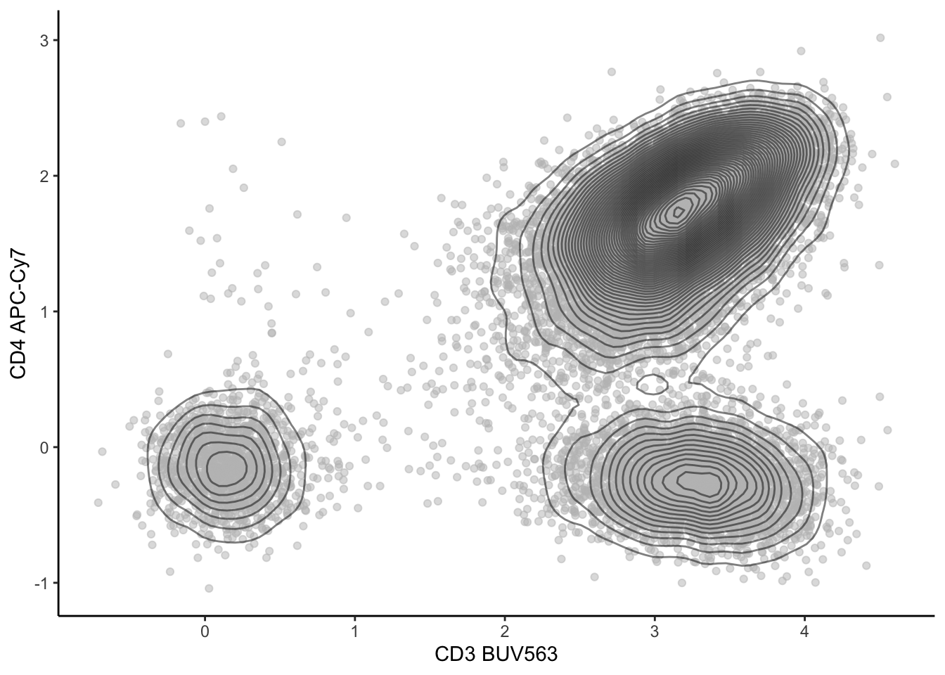

Past versions of unnamed-chunk-17-2.png

Version	Author	Date
2c16dc0	DrThomasOneil	2025-04-28

# A contour plot of CD3 and CD4 expression over a density plot.
ILC_transf %>%
  ggplot(aes(x = CD3, y = CD4))+        
  geom_bin_2d(bins = 200)+
  scale_fill_gradientn(colors = c("blue",  "yellow", "red"))+
  geom_density_2d(colour = "black")+
  xlab("CD3 BUV563")+
  ylab("CD4 APC-Cy7")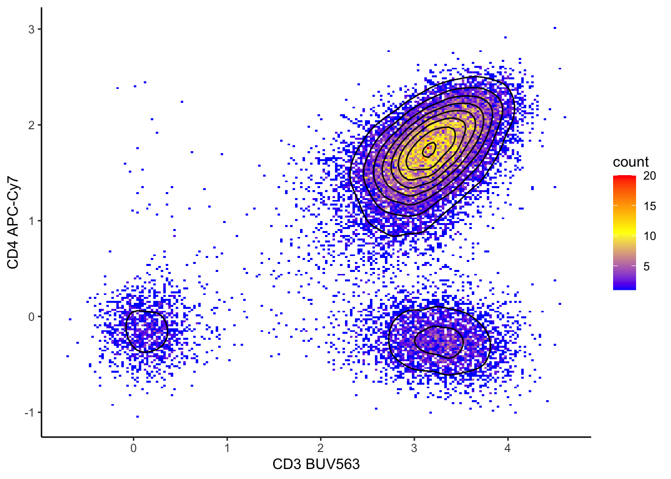

Past versions of unnamed-chunk-17-3.png

Version	Author	Date
2c16dc0	DrThomasOneil	2025-04-28

Subsetting data and summary statistics

While not as efficient as FlowJo, we can subset data after exporting. We wouldn’t normally do this in R, but we’ll show you how you could subset in R and for the purposes of visualisation.

Subsetting

# Plot a 2-marker plot of CD3 and CD4 expression values. 
ILC_transf %>%
  ggplot(aes(x = CD3, y = CD4))+        
  geom_bin_2d(bins = 200)+
  scale_fill_gradientn(colors = c("blue",  "yellow", "red"))+
  xlab("CD3 BUV563")+
  ylab("CD4 APC-Cy7")+
  geom_vline(xintercept = 1.3)+ #choose the x intercept
  geom_hline(yintercept = 0.6)  #choose the y intercept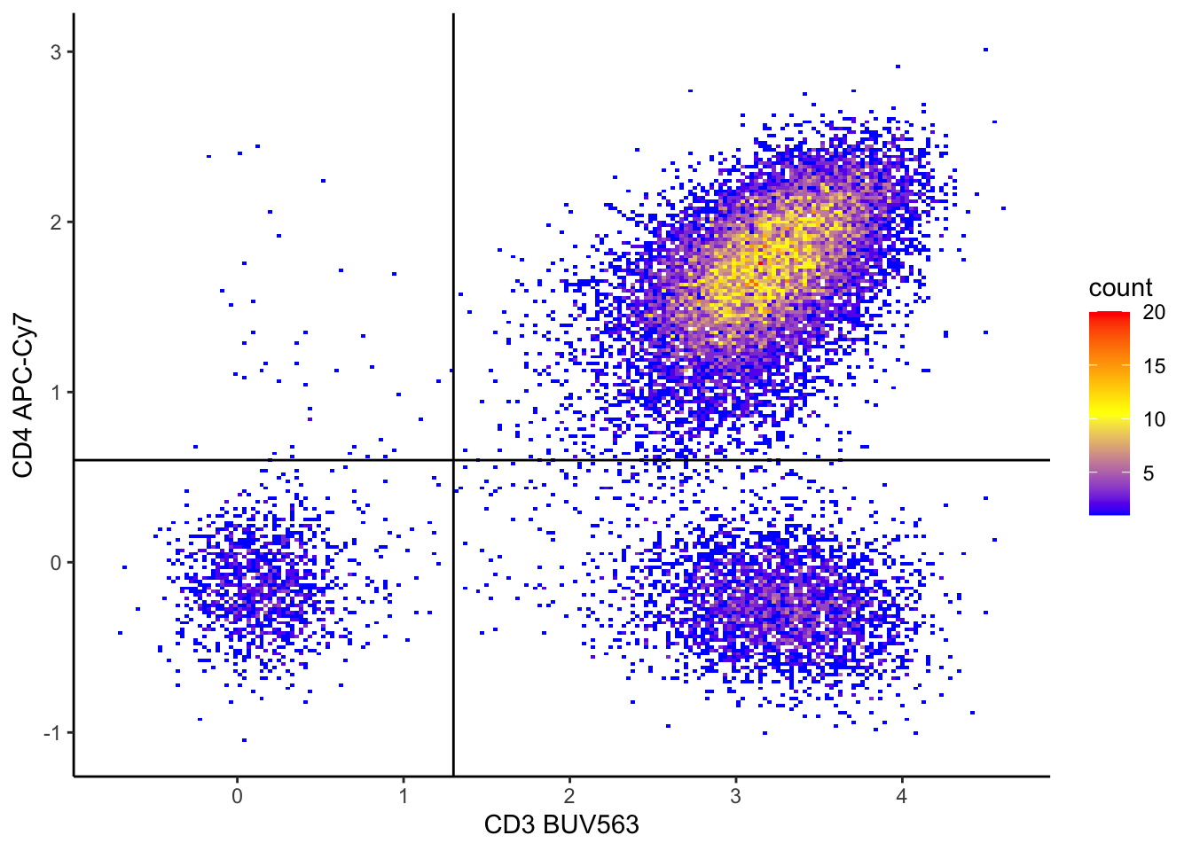

Past versions of unnamed-chunk-18-1.png

Version	Author	Date
2c16dc0	DrThomasOneil	2025-04-28

Subset the dataset based on these thresholds.

# This code creates a new column named 'subset' in the 'ILC_transf' dataset.
# The 'subset' column categorises rows based on the values of 'CD3' and 'CD4' columns:
# - "CD3+CD4+": if CD3 > 1.3 and CD4 > 0.6
# - "CD3+CD4-": if CD3 > 1.3 and CD4 <= 0.6
# - "CD3-CD4+": if CD3 <= 1.3 and CD4 > 0.6
# - "CD3-CD4-": if CD3 <= 1.3 and CD4 <= 0.6
# The 'mutate' function from the dplyr package is used to add this new column.

ILC_transf <- ILC_transf %>% 
  mutate(subset = case_when(
    CD3 > 1.3 & CD4 > 0.6 ~ "CD3+CD4+",
    CD3 > 1.3 & CD4 <= 0.6 ~ "CD3+CD4-",
    CD3 <= 1.3 & CD4 > 0.6 ~ "CD3-CD4+",
    TRUE ~ "CD3-CD4-"
  ))

Visualise the subsets in dot plots

ILC_transf %>%
  ggplot(aes(x = CD3, y = CD4, color=subset))+        
  geom_point()+
  xlab("CD3 BUV563")+
  ylab("CD4 APC-Cy7")+geom_vline(xintercept = 1.3)+
  geom_hline(yintercept = 0.6)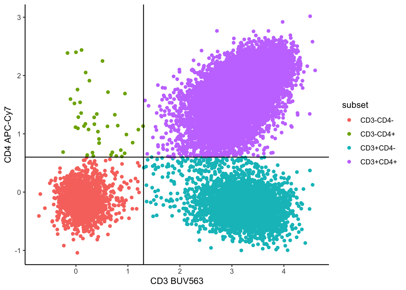

Past versions of unnamed-chunk-20-1.png

Version	Author	Date
2c16dc0	DrThomasOneil	2025-04-28
ec75f7d	DrThomasOneil	2025-04-26

# Look at different markers coloured by subset
ILC_transf %>%
  ggplot(aes(x = CD56, y = CD16, color=subset))+        
  geom_point()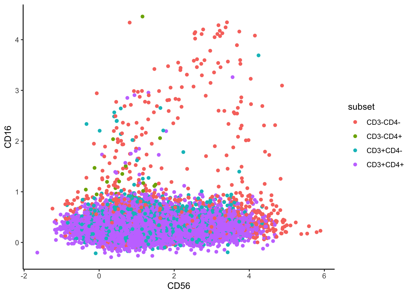

Past versions of unnamed-chunk-20-2.png

Version	Author	Date
2c16dc0	DrThomasOneil	2025-04-28
ec75f7d	DrThomasOneil	2025-04-26

# Split by subset
ILC_transf %>%
  ggplot(aes(x =CD56, y = CD16))+        
  geom_bin_2d(bins = 200)+
  scale_fill_gradientn(colors = c("blue",  "yellow", "red"))+
  facet_wrap(~subset)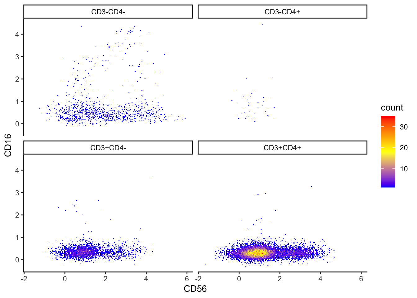

Past versions of unnamed-chunk-20-3.png

Version	Author	Date
2c16dc0	DrThomasOneil	2025-04-28

ILC_transf %>%
  ggplot(aes(x =FSC.A, y = SSC.A))+        
  geom_bin_2d(bins = 200)+
  scale_fill_gradientn(colors = c("blue",  "yellow", "red"))+
  facet_wrap(~subset)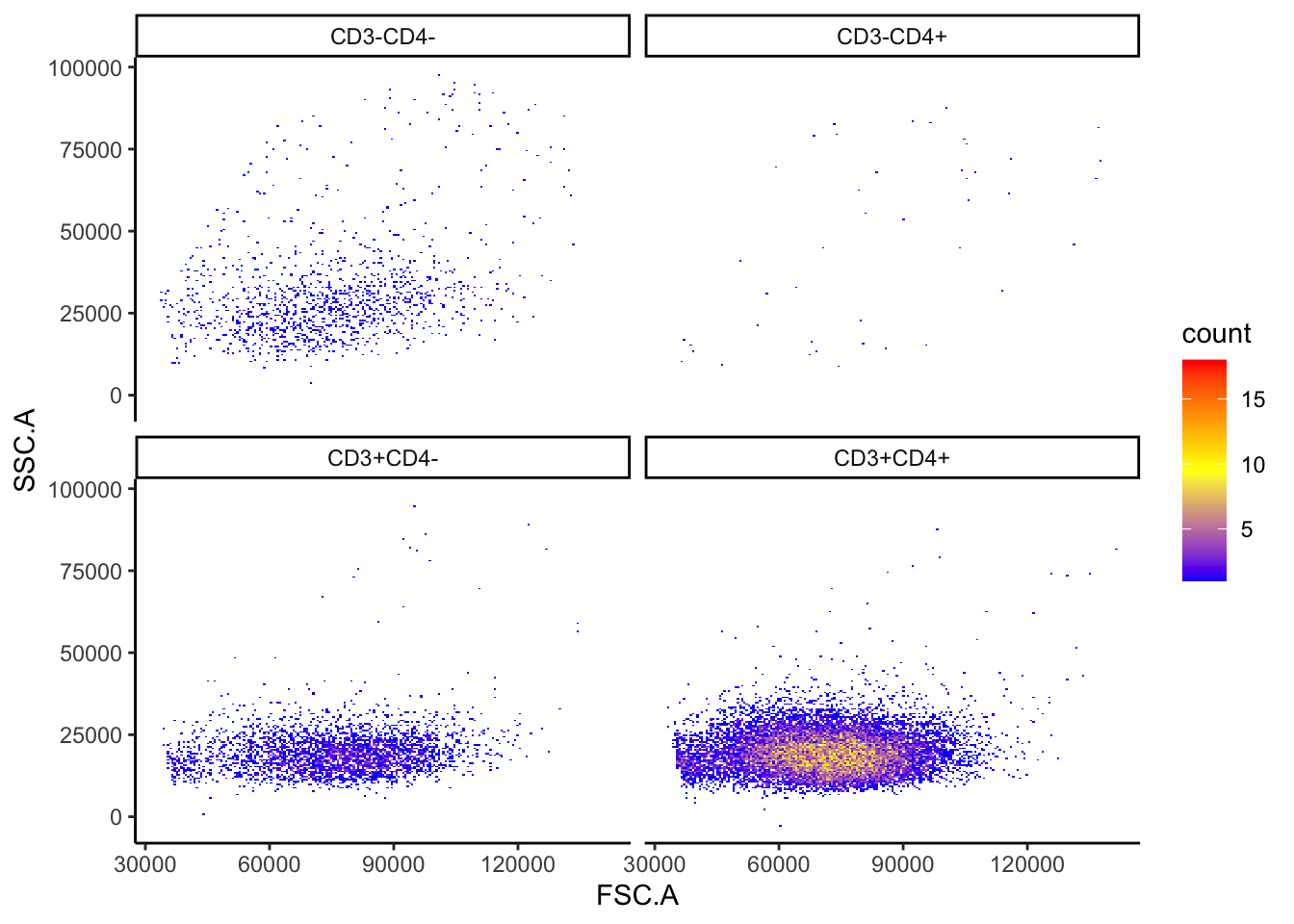

Past versions of unnamed-chunk-20-4.png

Version	Author	Date
2c16dc0	DrThomasOneil	2025-04-28

Histograms

ILC_transf %>%
  ggplot(aes(x = CD56, color = subset, fill = subset)) +
  geom_density(alpha = 0.2, linewidth = 1)+
  xlim(quantile(ILC_transf$CD56, 0.001),quantile(ILC_transf$CD56, 0.999))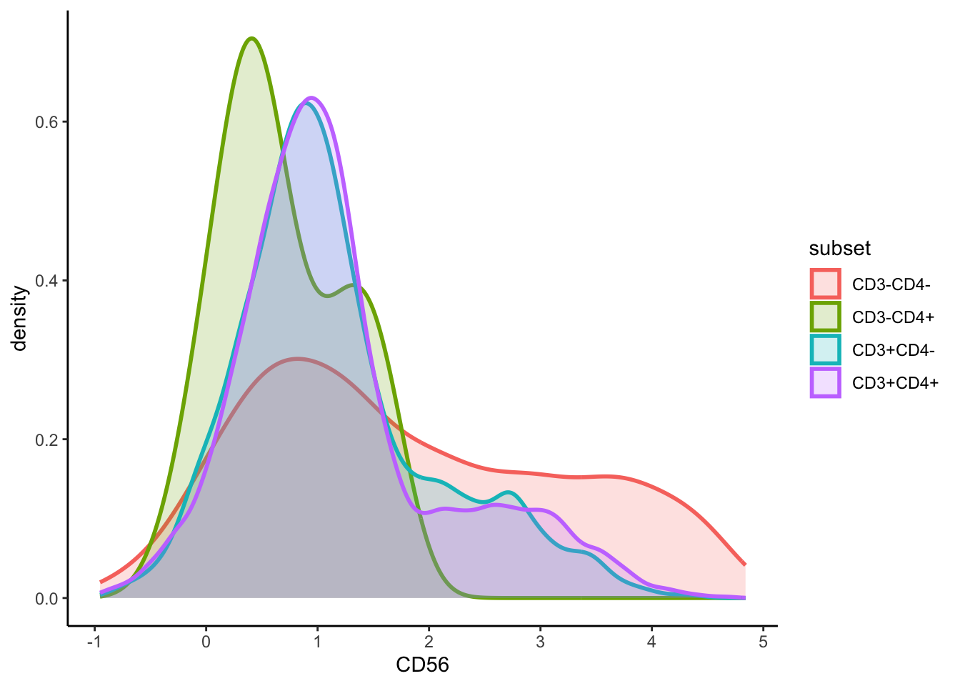

Past versions of unnamed-chunk-21-1.png

Version	Author	Date
2c16dc0	DrThomasOneil	2025-04-28
ec75f7d	DrThomasOneil	2025-04-26

#using ggridges
ILC_transf %>%
  ggplot(aes(x = CD56, y = subset, fill = subset)) +
  geom_density_ridges(scale = 1.2, alpha = 0.6, colour = "black") +
  theme_ridges() +
  theme(legend.position = "none")+
  labs(y="", x="", title = "CD56")+
  xlim(quantile(ILC_transf$CD56, 0.001),quantile(ILC_transf$CD56, 0.999))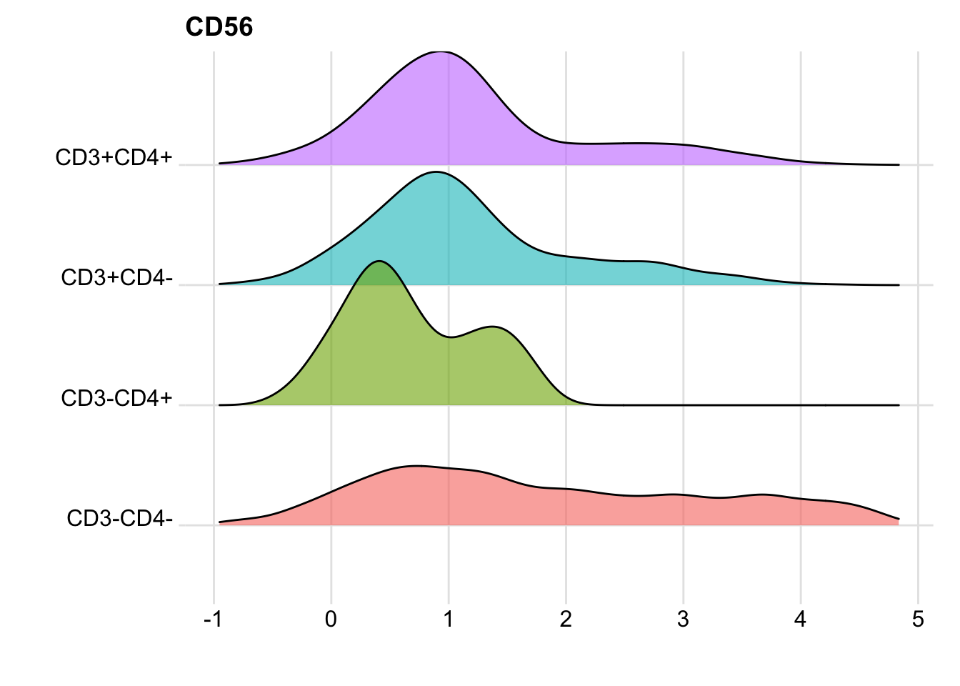

Past versions of unnamed-chunk-21-2.png

Version	Author	Date
2c16dc0	DrThomasOneil	2025-04-28

You could mass print these using a loop, as we did for the density plots above. You can also adjust the marker you output, as not all markers or combinations of markers are useful.

Summary statistics

While subsetting is not as efficient as FlowJo, summarising data is!

We can first collect subset percentages and output them in a table, in text, and even in a plot. Then we can calculate summary statistics like MFI & gMFI.

# total summary
round(table(ILC_transf$subset)*100/nrow(ILC_transf),2) # % of each subset

CD3-CD4- CD3-CD4+ CD3+CD4- CD3+CD4+ 
    6.56     0.22    17.79    75.44 

# individual marker
ILC_transf %>% 
  group_by(subset) %>% 
  summarise(Percent = round(n()/nrow(ILC_transf)*100,2)) %>%
  mutate(subset = factor(subset, levels = c("CD3+CD4+", "CD3+CD4-", "CD3-CD4+", "CD3-CD4-")))%>%
  mutate(Subsets = "Subsets") %>%
  ggplot(aes(x=Subsets,y = Percent, fill = subset)) +
    geom_bar(stat = "identity", show.legend = FALSE) +
    ylab("Percentage") +
    xlab("") +
    scale_fill_manual(values = c("CD3+CD4+" = "blue", "CD3+CD4-" = "red", "CD3-CD4+" = "green", "CD3-CD4-" = "yellow")) +
    theme(axis.text.x = element_blank(), axis.ticks.x = element_blank()) +
    theme(axis.text.y = element_text(size=10)) +
    theme(legend.position = "none") +
    theme(plot.title = element_text(hjust = 0.5, size=10)) +
    ggtitle("Subsets of CD3+/-CD4+/- cells")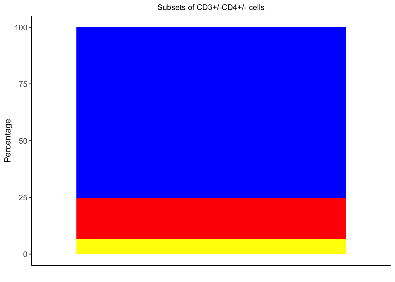

Past versions of unnamed-chunk-22-1.png

Version	Author	Date
2c16dc0	DrThomasOneil	2025-04-28

We can also calculate the percentage of subsets in line, meaning we don’t have to change these lines of text based on different results or different data:

• CD3+CD4+: 75.44%

• CD3+CD4-: 17.79%

• CD3-CD4+: 0.22%

• CD3-CD4-: 6.56%

You can also quickly calculate summary statistics like MFI, gMFI, medianFI:

Arithmatic MFI

ILC$subset  <- ILC_transf$subset # Add the subset column to the original data.

ILC %>% 
  group_by(subset) %>% 
  summarise(across(7:31, mean, .names = "MFI_{col}"))
# A tibble: 4 × 26
  subset  MFI_NKp44 MFI_Lineage MFI_CD45 MFI_CD103 MFI_FVS700 MFI_CD4 MFI_HLA.DR
  <chr>       <dbl>       <dbl>    <dbl>     <dbl>      <dbl>   <dbl>      <dbl>
1 CD3+CD…      49.9        119.    9901.      591.     -40.0   1419.        176.
2 CD3+CD…      55.5        131.   10543.      865.     -42.8   -115.        193.
3 CD3-CD…     113.         491.    6915.      431.      -5.70   918.      15030.
4 CD3-CD…     250.         242.    4114.     1158.     -64.6    -69.4      1247.
# ℹ 18 more variables: MFI_CD16 <dbl>, MFI_CD3 <dbl>, MFI_CD94 <dbl>,
#   MFI_CD39 <dbl>, MFI_CD56 <dbl>, MFI_TCRVA72 <dbl>, MFI_CKIT <dbl>,
#   MFI_CD14.CD19 <dbl>, MFI_CD49D <dbl>, MFI_CD244 <dbl>, MFI_CD161 <dbl>,
#   MFI_TCRgt <dbl>, MFI_CD69 <dbl>, MFI_CD25 <dbl>, MFI_ITAGB7 <dbl>,
#   MFI_CRTH2 <dbl>, MFI_NKp46 <dbl>, MFI_CD127 <dbl>

Median FI

ILC %>% 
  group_by(subset) %>% 
  summarise(across(7:31, median, .names = "MFI_{col}"))
# A tibble: 4 × 26
  subset  MFI_NKp44 MFI_Lineage MFI_CD45 MFI_CD103 MFI_FVS700 MFI_CD4 MFI_HLA.DR
  <chr>       <dbl>       <dbl>    <dbl>     <dbl>      <dbl>   <dbl>      <dbl>
1 CD3+CD…      45.0        109.    9679.      403.     -39.6   1356.        133.
2 CD3+CD…      49.6        115.   10416.      595.     -38.9   -122.        135.
3 CD3-CD…     105.         541.    5582.      380.      -1.28   695.       3534.
4 CD3-CD…     176.         201.    3898.      243.     -58.6    -71.0       266.
# ℹ 18 more variables: MFI_CD16 <dbl>, MFI_CD3 <dbl>, MFI_CD94 <dbl>,
#   MFI_CD39 <dbl>, MFI_CD56 <dbl>, MFI_TCRVA72 <dbl>, MFI_CKIT <dbl>,
#   MFI_CD14.CD19 <dbl>, MFI_CD49D <dbl>, MFI_CD244 <dbl>, MFI_CD161 <dbl>,
#   MFI_TCRgt <dbl>, MFI_CD69 <dbl>, MFI_CD25 <dbl>, MFI_ITAGB7 <dbl>,
#   MFI_CRTH2 <dbl>, MFI_NKp46 <dbl>, MFI_CD127 <dbl>

Geometric MFI

The traditional formula written out would be like ILC_transf %>% prod(CD56)^(1/nrow(CD56)). However, as our data is compensated, there are meaningful negative values and 0s that we don’t want to get rid of, which if you run on this data removes two subsets entirely. FlowJo calculates the graph spaces as gMFI to enable it to deal with negatives and 0s. Here in this case, it may be better to stick with the arithmetic mean instead of forcing the geometric mean.

nxn plots

You can also create a loop to view the nxn plots, and save them to the folder of your choice.

# Select only numeric marker columns
marker_cols <- colnames(ILC_transf)[1:25] # adjust if needed

# Make a customised function for plot streamline
custom_bin_plot <- function(data, mapping, ...) {
  ggplot(data = data, mapping = mapping) +
    geom_bin_2d(bins = 50) +
    scale_fill_gradientn(colours = c("blue", "yellow", "red")) +
    theme_minimal()
}

# Generate plots
p <- ggpairs(
  ILC_transf,
  columns = marker_cols,
  lower = list(continuous = custom_bin_plot),
  diag = list(continuous = wrap("densityDiag", alpha = 0.4)),
  upper = list(continuous = wrap("cor", size = 3))
)
ggsave("plots/nxn.png",p, width=25, height=25,unit="in")

rm(p,custom_bin_plot, marker_cols)

Dimension reduction and clustering

There are several ways to perform clustering (e.g. FlowSOM, FuseSOM) and dimension reduction (e.g. PCA, UMAP, tSNE).

In this section, we’ll cover clustering and dimension reduction on our one sample.

Clustering

Clustering groups our cells based on the input expressions we choose.

FlowSOM

Read more

# Perform clustering
clusters <- FlowSOM::FlowSOM(
  input=as.matrix(ILC_transf[,1:32]),
  silent = FALSE,
  colsToUse = c(1,4,6:14,16:25),
  nClus = 15)

# Annotate the cluster that the cell belongs to
ILC_transf$flowSOM<- GetMetaclusters(clusters)
#FlowSOM::GetMetaclusterMFIs(clusters)

# Plot CD4 expression values on clusters
ILC_transf %>%
  ggplot(aes(x = CD56, y = flowSOM, fill = flowSOM)) +
  geom_density_ridges(scale = 1.2, alpha = 0.6, colour = "black") +
  theme_ridges() +
  theme(legend.position = "none")+
  labs(y="", x="", title = "CD56")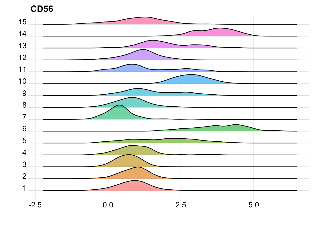

Past versions of unnamed-chunk-26-1.png

Version	Author	Date
94e37b3	DrThomasOneil	2025-04-28
2c16dc0	DrThomasOneil	2025-04-28
ec75f7d	DrThomasOneil	2025-04-26

FuseSOM

Read more

risomMarkers <- colnames(ILC_transf)[c(1,4,6:14,16:25)]
clusters <- runFuseSOM(data = as.matrix(ILC_transf[,1:32]), 
                       markers = risomMarkers, 
                       numClusters = 15)

ILC_transf$fuseSOM<- as.numeric(unlist(lapply(str_split(clusters$clusters, "_"), function(x) x[[2]])))

ILC_transf %>%
  ggplot(aes(x = CD56, y = as.factor(fuseSOM), fill=as.factor(fuseSOM))) +
  geom_density_ridges(scale = 1.2, alpha = 0.6, colour = "black") +
  theme_ridges() +
  theme(legend.position = "none")+
  labs(y="", x="", title = "CD56")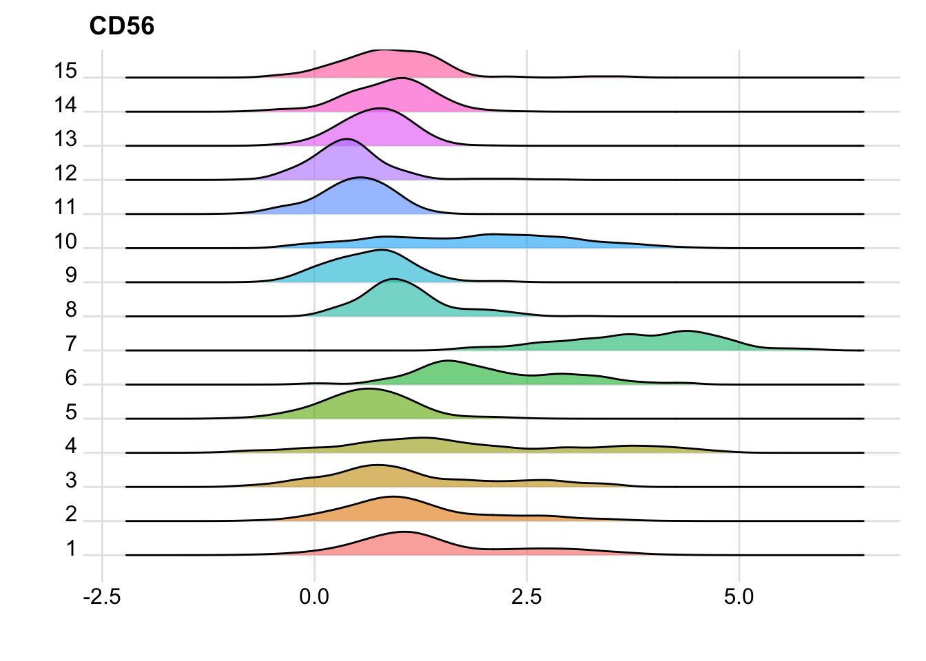

Past versions of unnamed-chunk-27-1.png

Version	Author	Date
2c16dc0	DrThomasOneil	2025-04-28

Dimension Reduction

We’ll generate a PCA, a tSNE and a UMAP. I’ll then run through all of this in the Spectre packge.

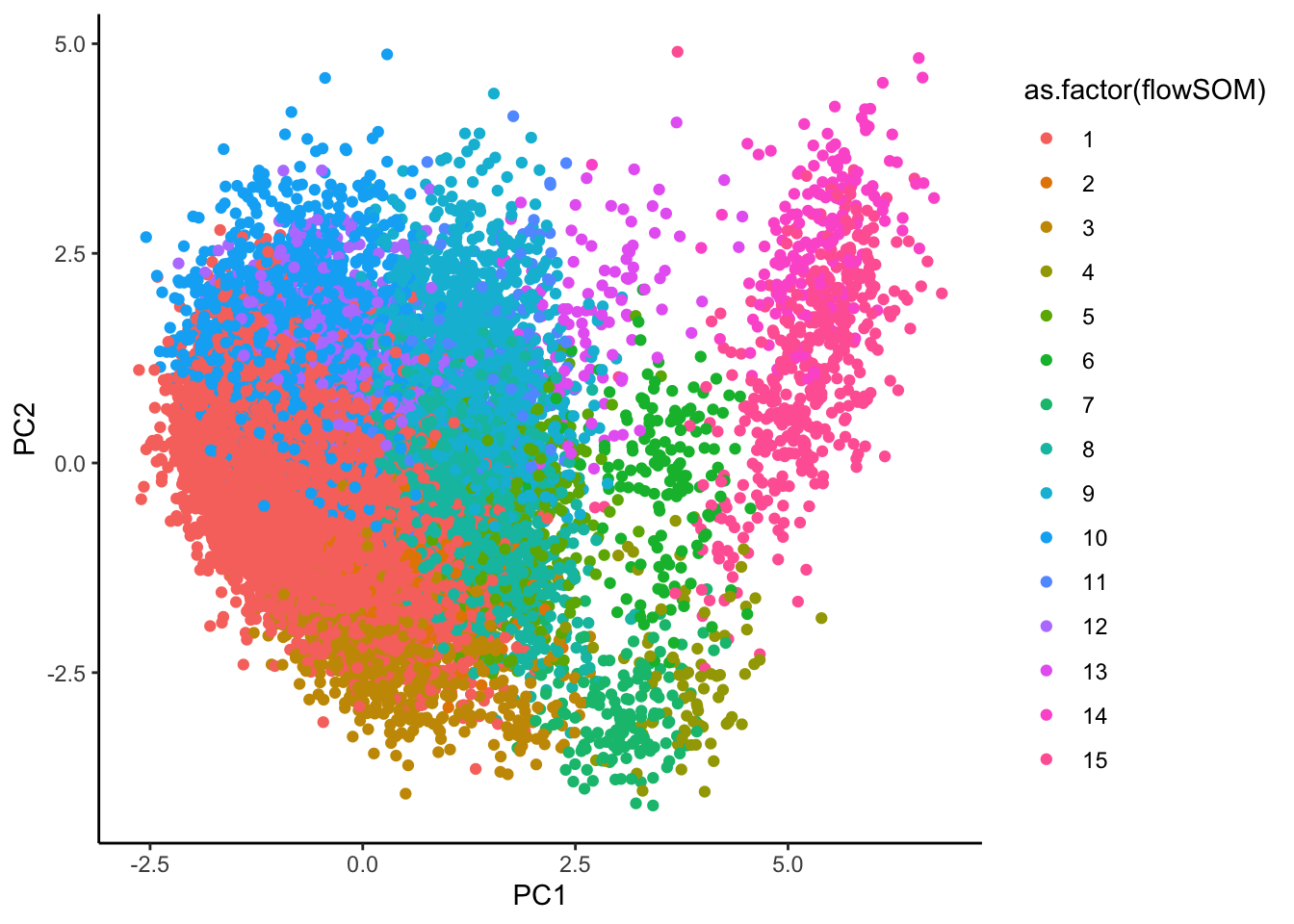
pca <- prcomp(as.matrix(ILC_transf[,c(1,4,6:14,16:25)]), center = TRUE)

ILC_transf <- ILC_transf %>% 
  mutate(PC1 = pca$x[,1],
         PC2 = pca$x[,2])

# can take a while
tsne <- Rtsne(as.matrix(ILC_transf[,c(1,4,6:14,16:25)]), dims = 2, perplexity = 30, verbose = TRUE)

Performing PCA
Read the 19588 x 21 data matrix successfully!
Using no_dims = 2, perplexity = 30.000000, and theta = 0.500000
Computing input similarities...
Building tree...
 - point 10000 of 19588
Done in 3.49 seconds (sparsity = 0.006800)!
Learning embedding...
Iteration 50: error is 104.675469 (50 iterations in 2.14 seconds)
Iteration 100: error is 103.985056 (50 iterations in 3.88 seconds)
Iteration 150: error is 96.379507 (50 iterations in 1.72 seconds)
Iteration 200: error is 95.668425 (50 iterations in 1.57 seconds)
Iteration 250: error is 95.464591 (50 iterations in 1.54 seconds)
Iteration 300: error is 4.105248 (50 iterations in 1.46 seconds)
Iteration 350: error is 3.820837 (50 iterations in 1.41 seconds)
Iteration 400: error is 3.652376 (50 iterations in 1.39 seconds)
Iteration 450: error is 3.532040 (50 iterations in 1.40 seconds)
Iteration 500: error is 3.441205 (50 iterations in 1.40 seconds)
Iteration 550: error is 3.369169 (50 iterations in 1.38 seconds)
Iteration 600: error is 3.310502 (50 iterations in 1.39 seconds)
Iteration 650: error is 3.261826 (50 iterations in 1.41 seconds)
Iteration 700: error is 3.220754 (50 iterations in 1.40 seconds)
Iteration 750: error is 3.185144 (50 iterations in 1.41 seconds)
Iteration 800: error is 3.153916 (50 iterations in 1.43 seconds)
Iteration 850: error is 3.126601 (50 iterations in 1.41 seconds)
Iteration 900: error is 3.102661 (50 iterations in 1.44 seconds)
Iteration 950: error is 3.081532 (50 iterations in 1.44 seconds)
Iteration 1000: error is 3.062794 (50 iterations in 1.43 seconds)
Fitting performed in 32.05 seconds.

ILC_transf <- ILC_transf %>% 
  mutate(tSNE1 = tsne$Y[,1],
         tSNE2 = tsne$Y[,2])

umap <- umap(ILC_transf[,c(1,4,6:14,16:25)])
ILC_transf <- ILC_transf %>% 
  mutate(UMAP1 = umap$layout[,1],
         UMAP2 = umap$layout[,2])

rm(pca,umap,tsne)

saveRDS(ILC_transf,"data/clustered_data.rds")

Visualisations

ILC_transf <- readRDS("data/clustered_data.rds")

ggplot(ILC_transf, aes(PC1,PC2, color= as.factor(flowSOM))) +
  geom_point()

Past versions of unnamed-chunk-31-1.png

Version	Author	Date
2c16dc0	DrThomasOneil	2025-04-28
ec75f7d	DrThomasOneil	2025-04-26

ggplot(ILC_transf, aes(tSNE1,tSNE2, color= as.factor(flowSOM))) +
  geom_point()

Past versions of unnamed-chunk-31-2.png

Version	Author	Date
2c16dc0	DrThomasOneil	2025-04-28
ec75f7d	DrThomasOneil	2025-04-26

ggplot(ILC_transf, aes(UMAP1,UMAP2, color= as.factor(flowSOM))) +
  geom_point()

Past versions of unnamed-chunk-31-3.png

Version	Author	Date
2c16dc0	DrThomasOneil	2025-04-28
ec75f7d	DrThomasOneil	2025-04-26

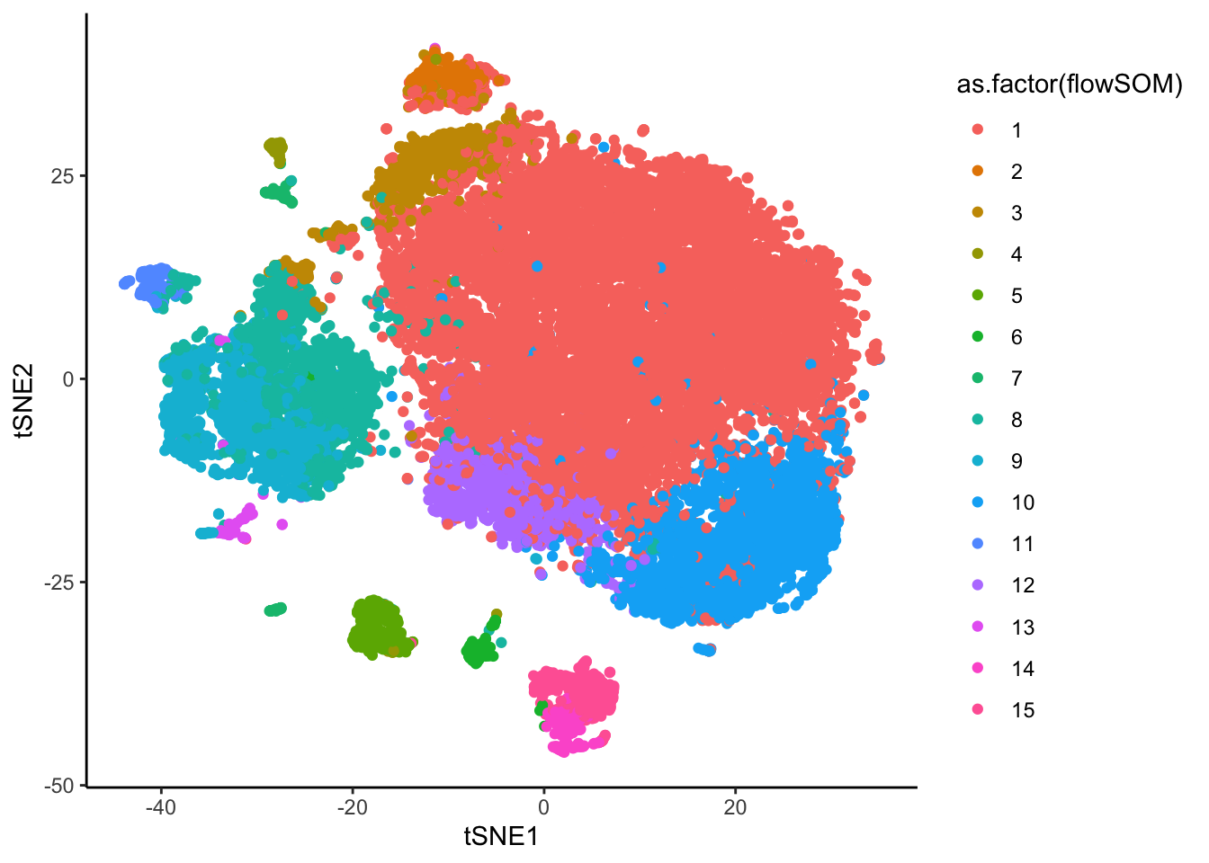
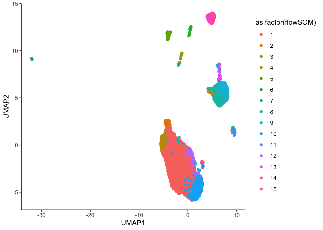
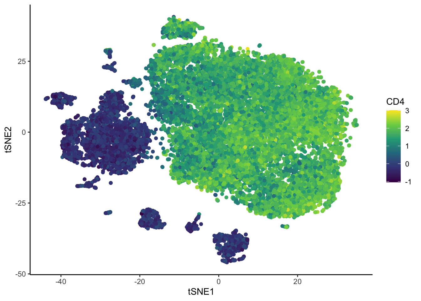
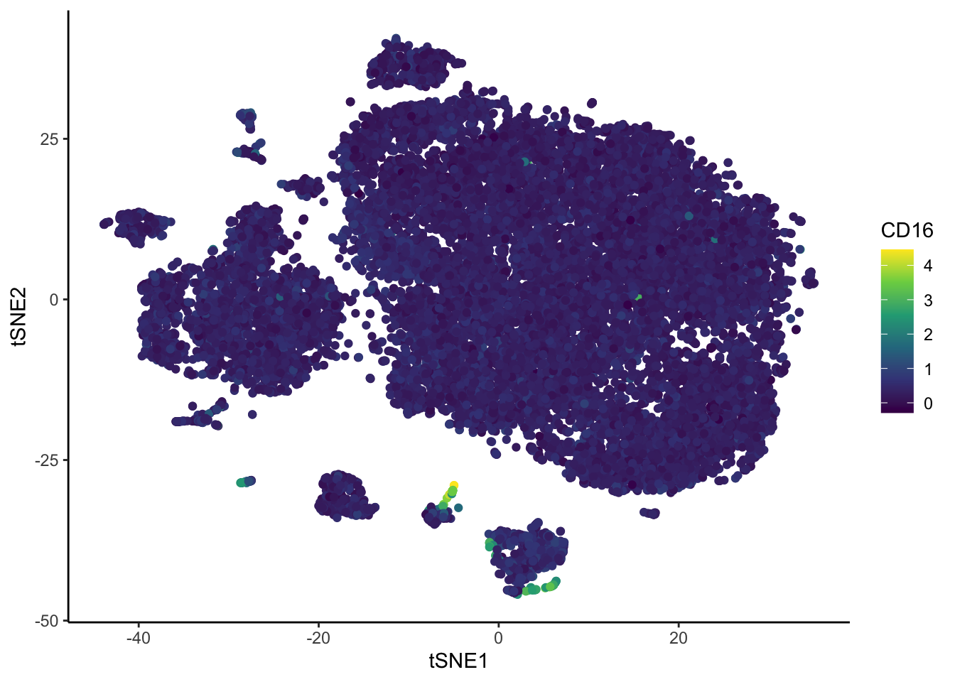
# Colour overlayed by the expression of one marker.
ggplot(ILC_transf, aes(tSNE1,tSNE2, color= CD3)) +
  geom_point() + 
  scale_color_viridis_c()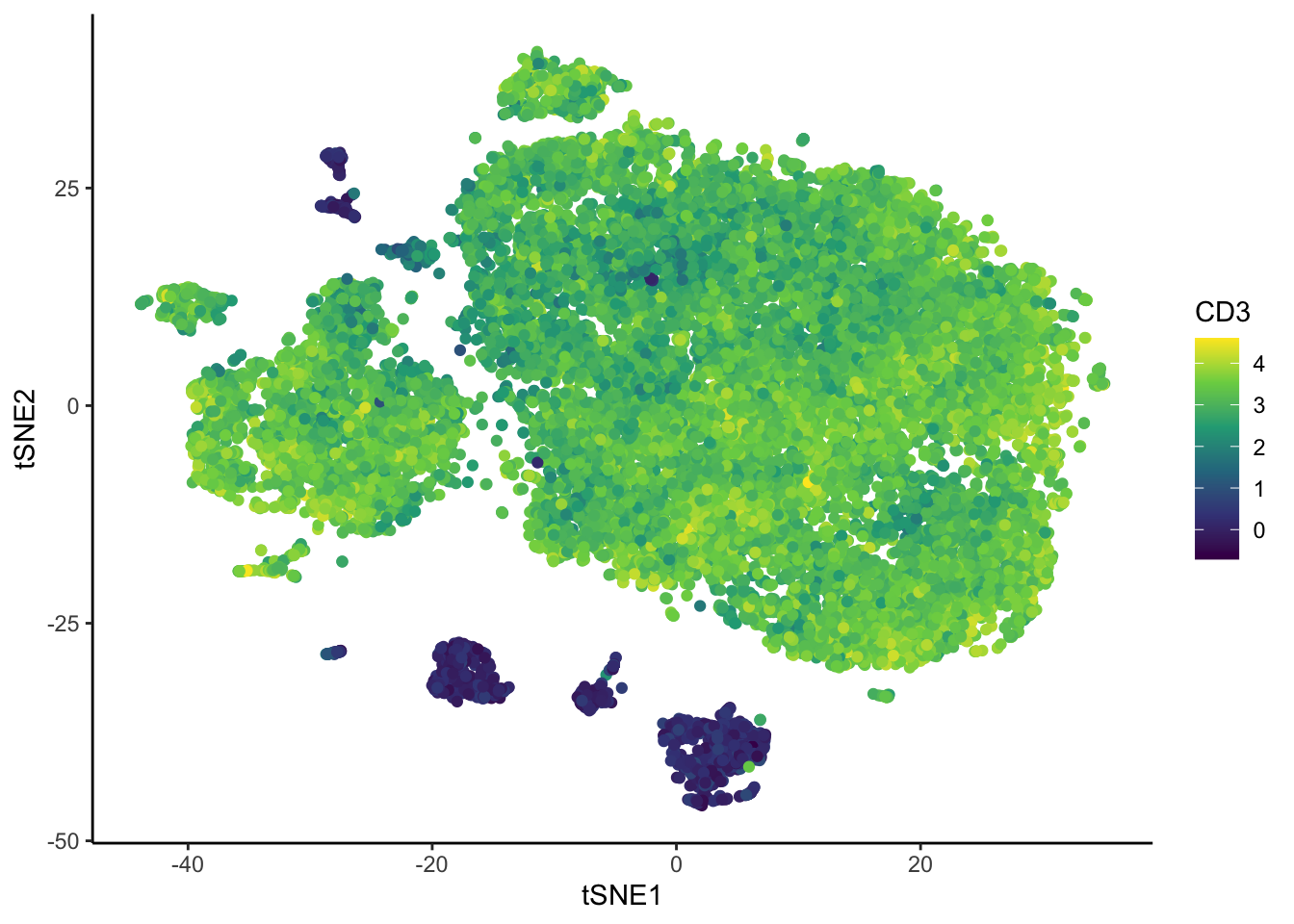

Past versions of unnamed-chunk-31-4.png

Version	Author	Date
2c16dc0	DrThomasOneil	2025-04-28
ec75f7d	DrThomasOneil	2025-04-26

ggplot(ILC_transf, aes(tSNE1,tSNE2, color= CD4)) +
  geom_point() + 
  scale_color_viridis_c()

Past versions of unnamed-chunk-31-5.png

Version	Author	Date
2c16dc0	DrThomasOneil	2025-04-28
ec75f7d	DrThomasOneil	2025-04-26

ggplot(ILC_transf, aes(tSNE1,tSNE2, color= CD16)) +
  geom_point() + 
  scale_color_viridis_c()

Past versions of unnamed-chunk-31-6.png

Version	Author	Date
2c16dc0	DrThomasOneil	2025-04-28
ec75f7d	DrThomasOneil	2025-04-26

Spectre

Read more

Spectre has easy plotting tools to visualize the results of clustering and dimension reduction.

make.colour.plot(ILC_transf, 
                 "tSNE1", "tSNE2", "subset",  
                 add.label = TRUE,
                 blank.axis = T,
                 path = "plots")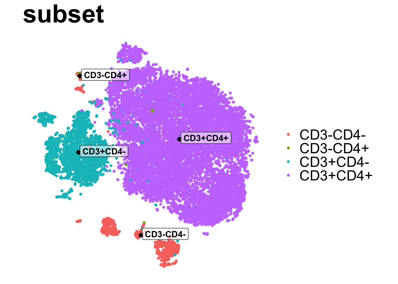

Past versions of unnamed-chunk-32-1.png

Version	Author	Date
2c16dc0	DrThomasOneil	2025-04-28

make.colour.plot(ILC_transf, 
                 "tSNE1", "tSNE2", "flowSOM", 
                 col.type = 'factor', 
                 add.label = TRUE,
                 blank.axis = T,
                 path = "plots")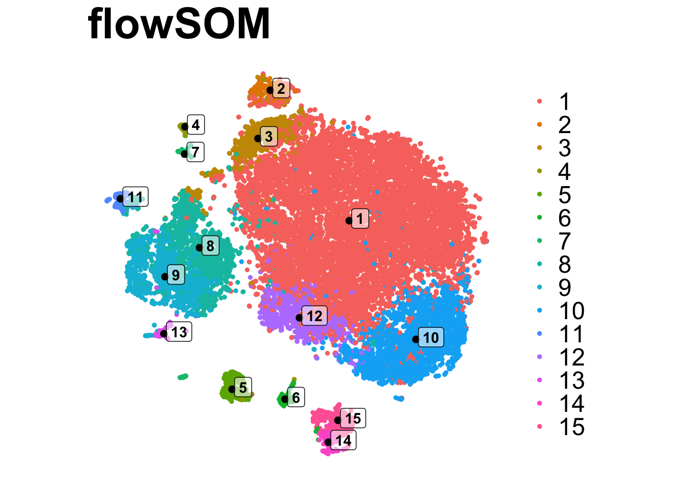

Past versions of unnamed-chunk-32-2.png

Version	Author	Date
2c16dc0	DrThomasOneil	2025-04-28

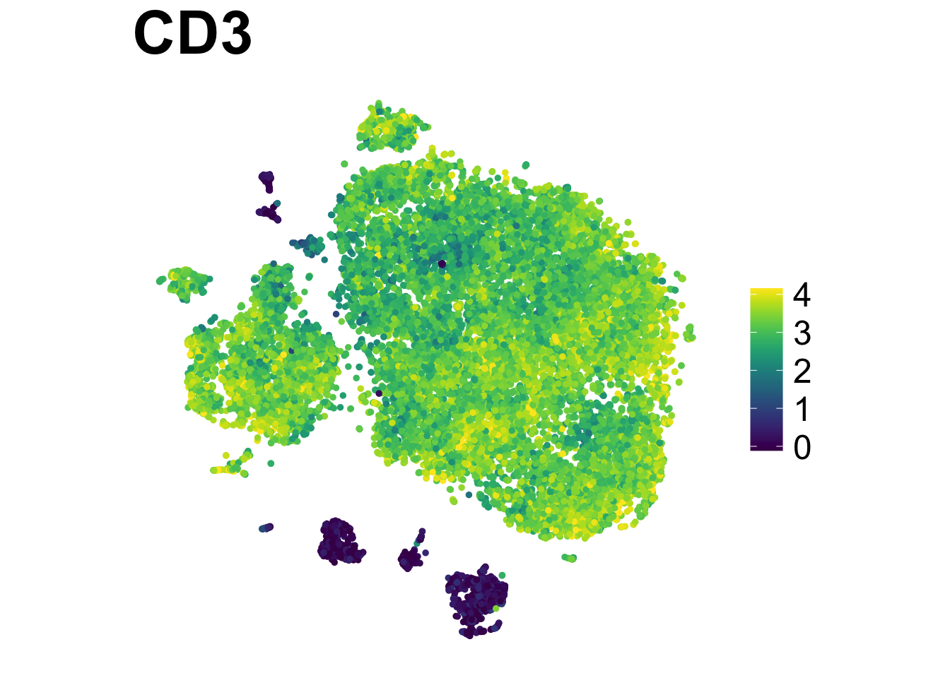
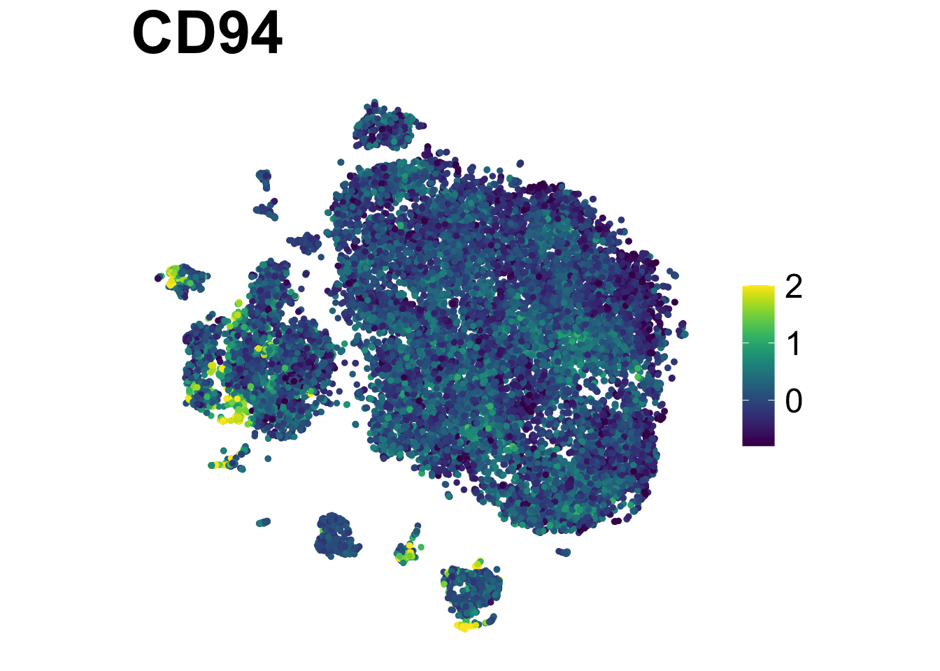
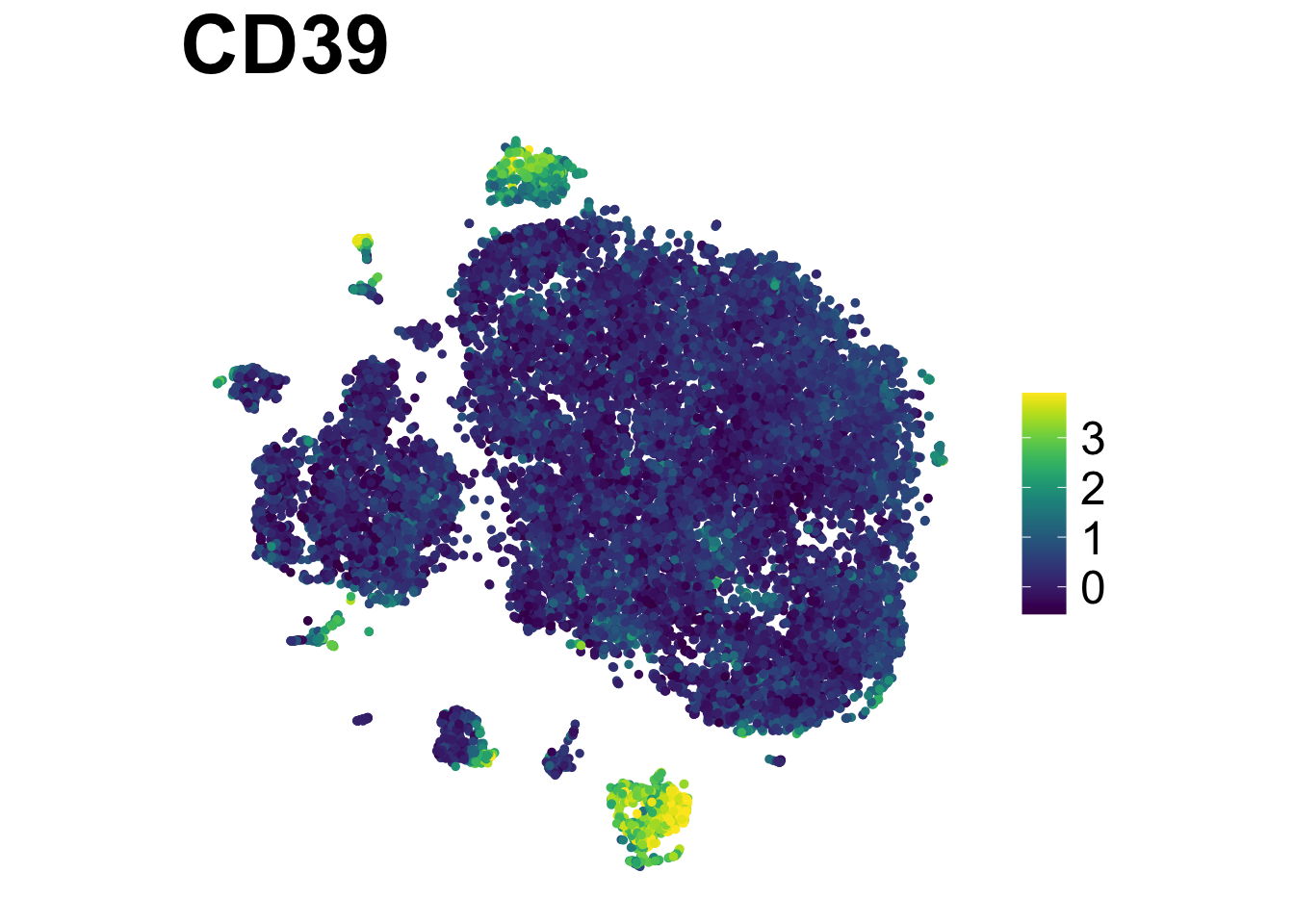
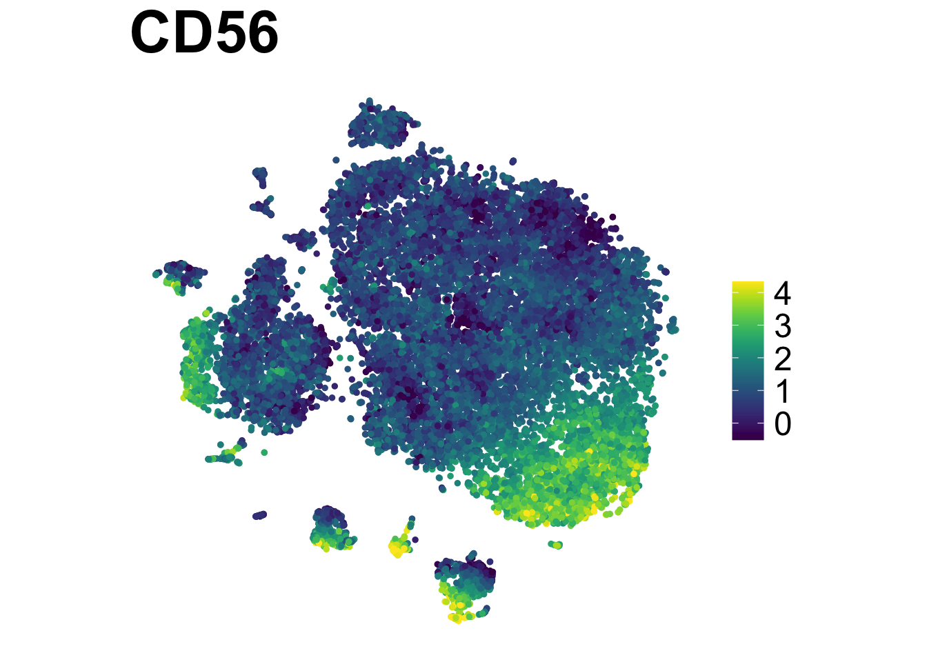
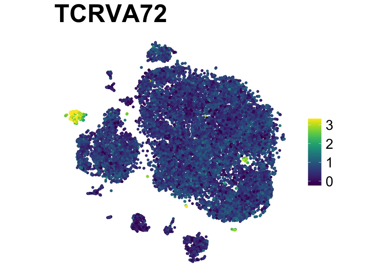
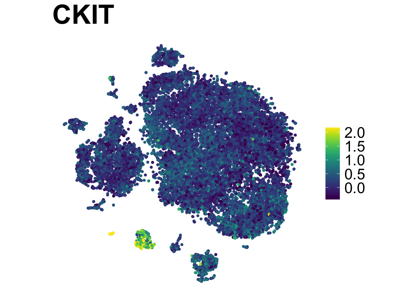
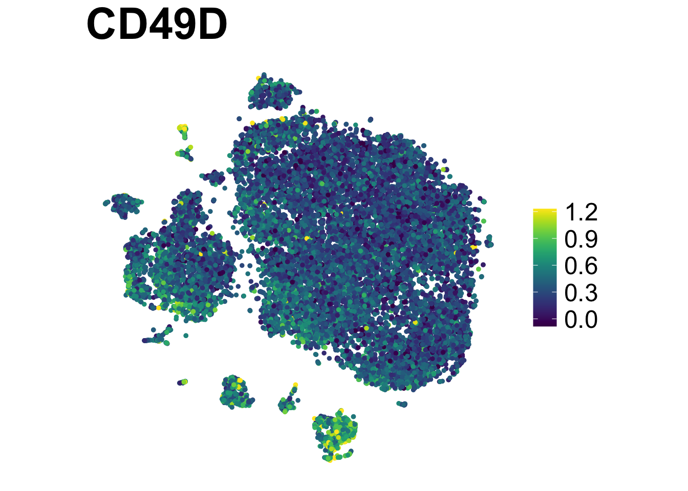
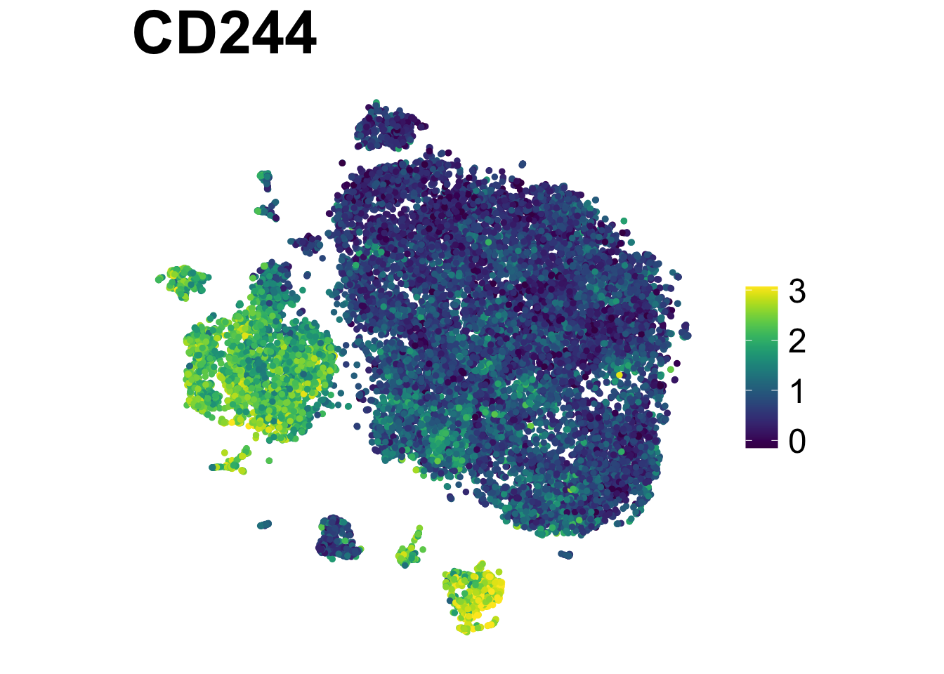
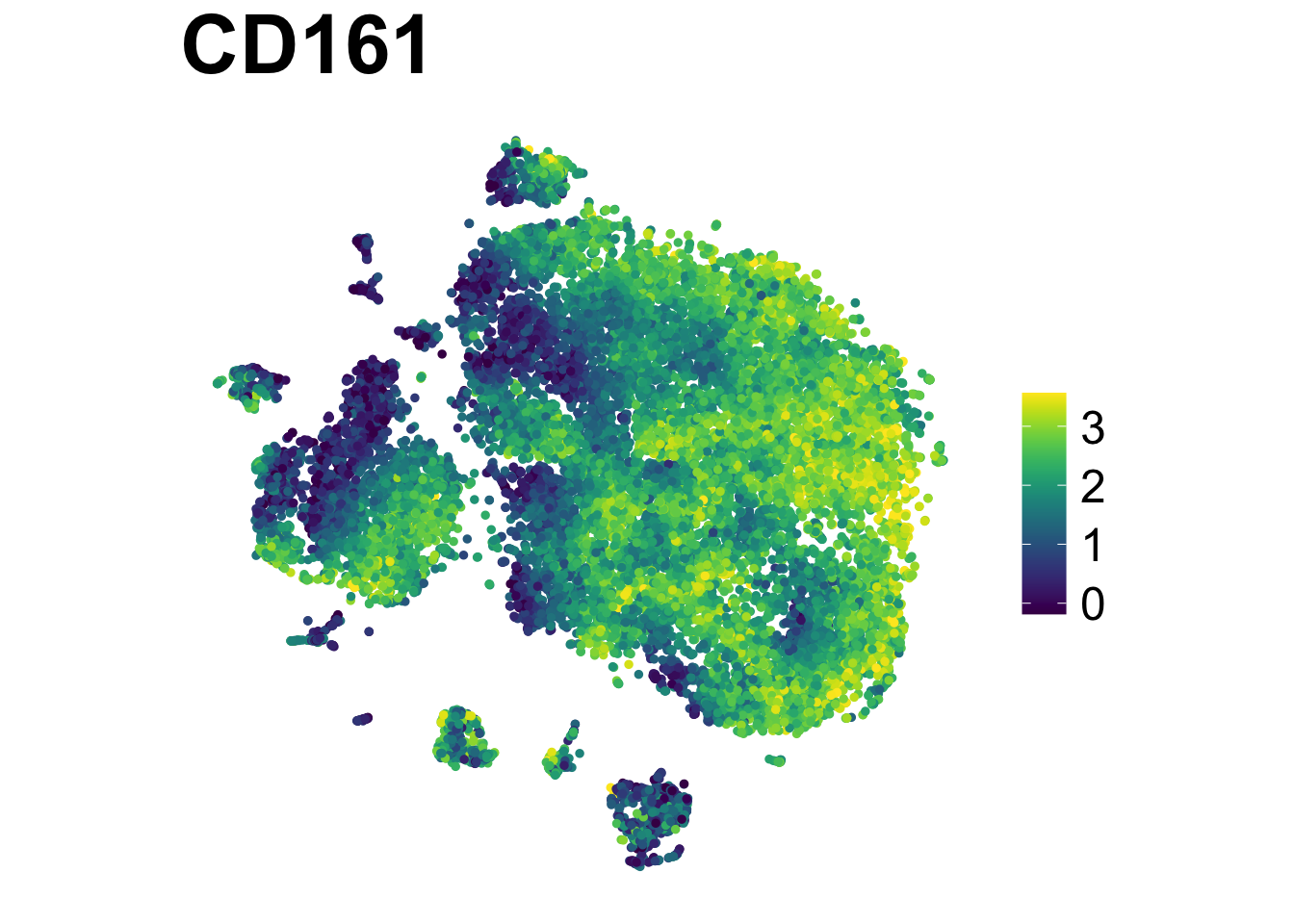
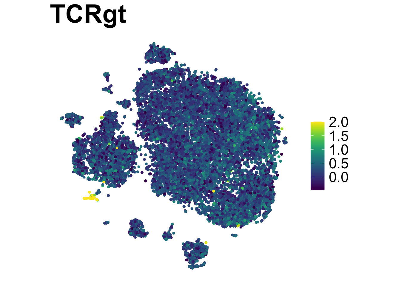
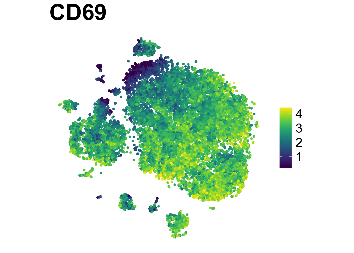
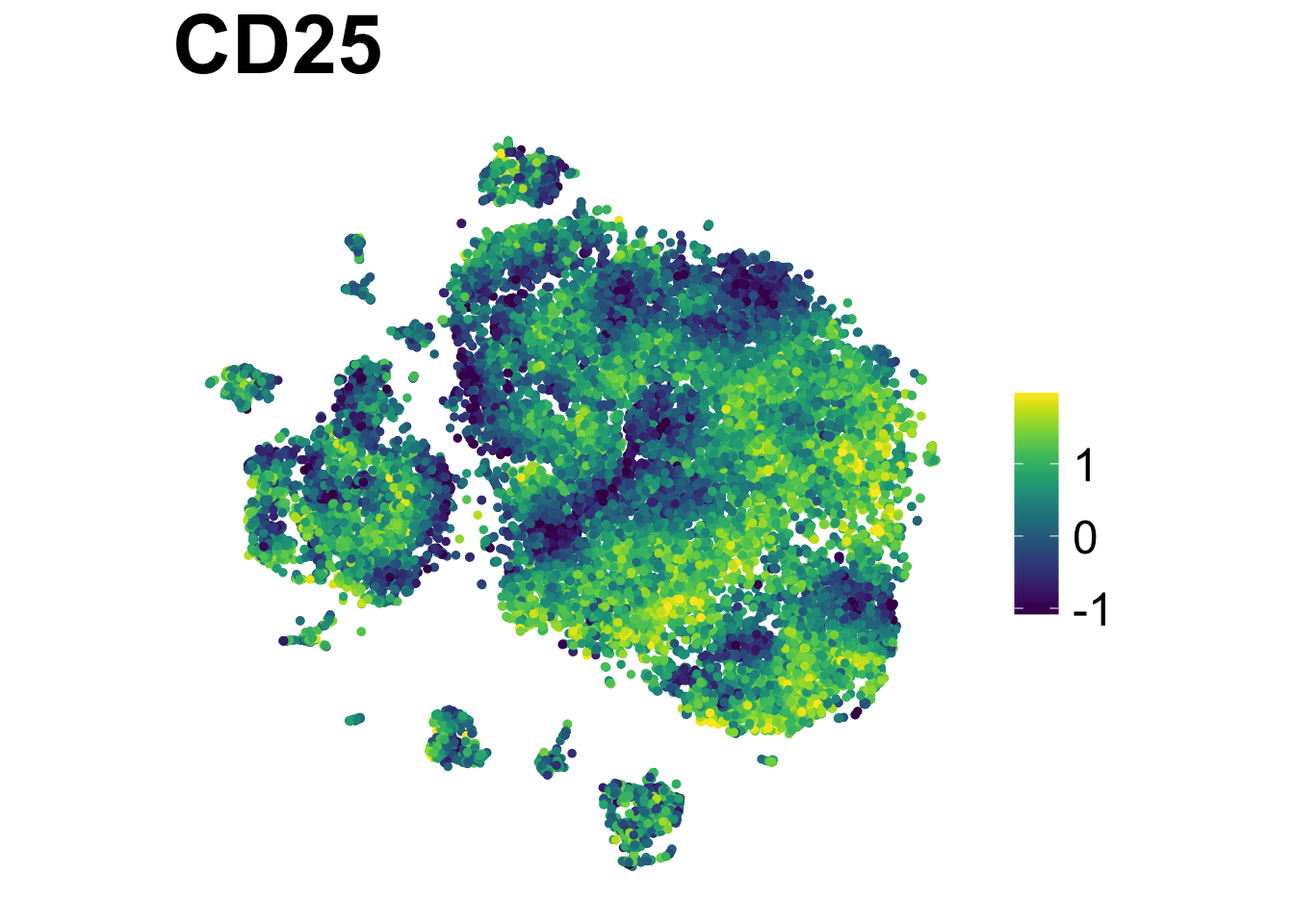
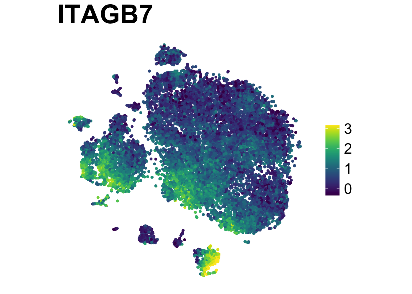
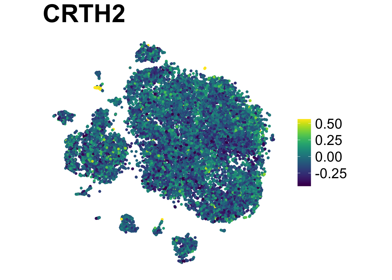
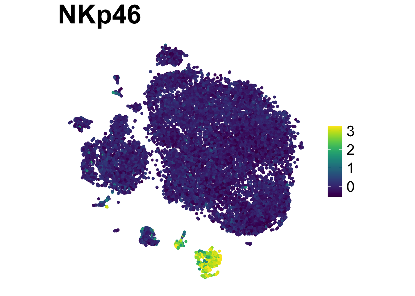
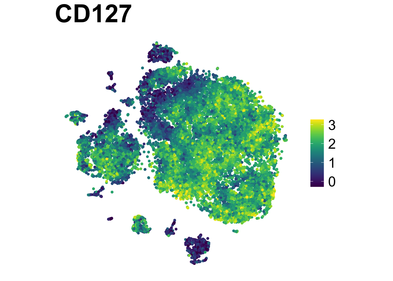
Multi-plots:

make.multi.plot(ILC_transf, 
                "tSNE1", "tSNE2", 
                risomMarkers, 
                blank.axis = T, 
                colours = "viridis", 
                path = "plots")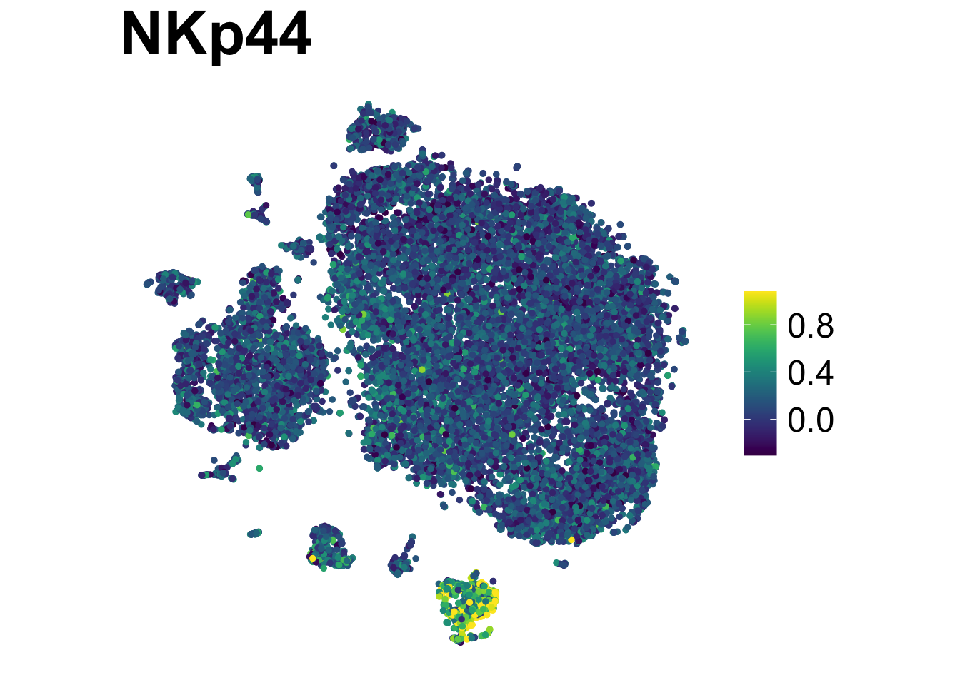

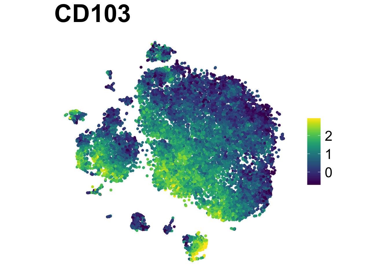
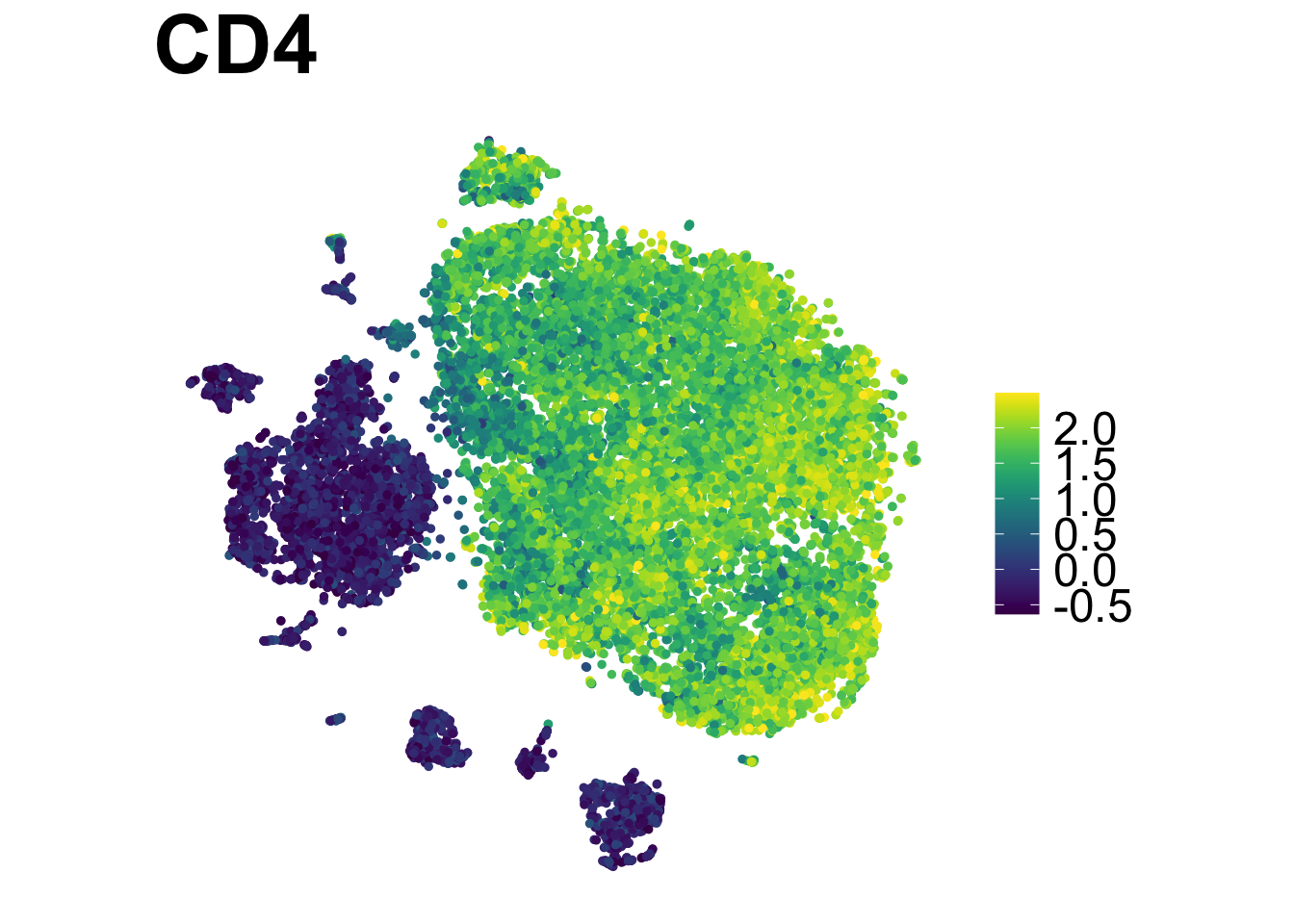
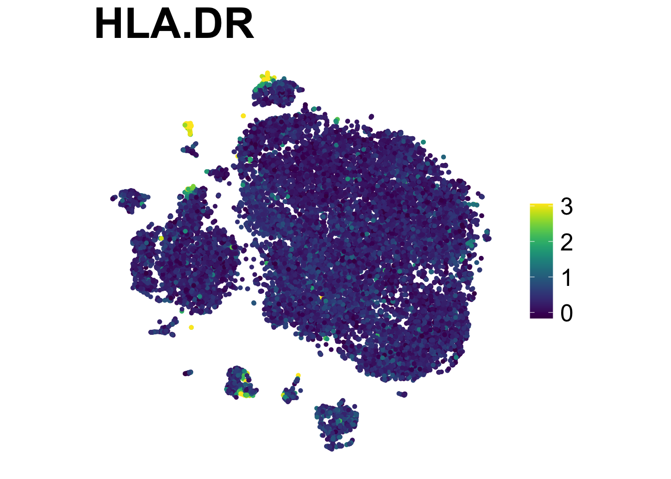
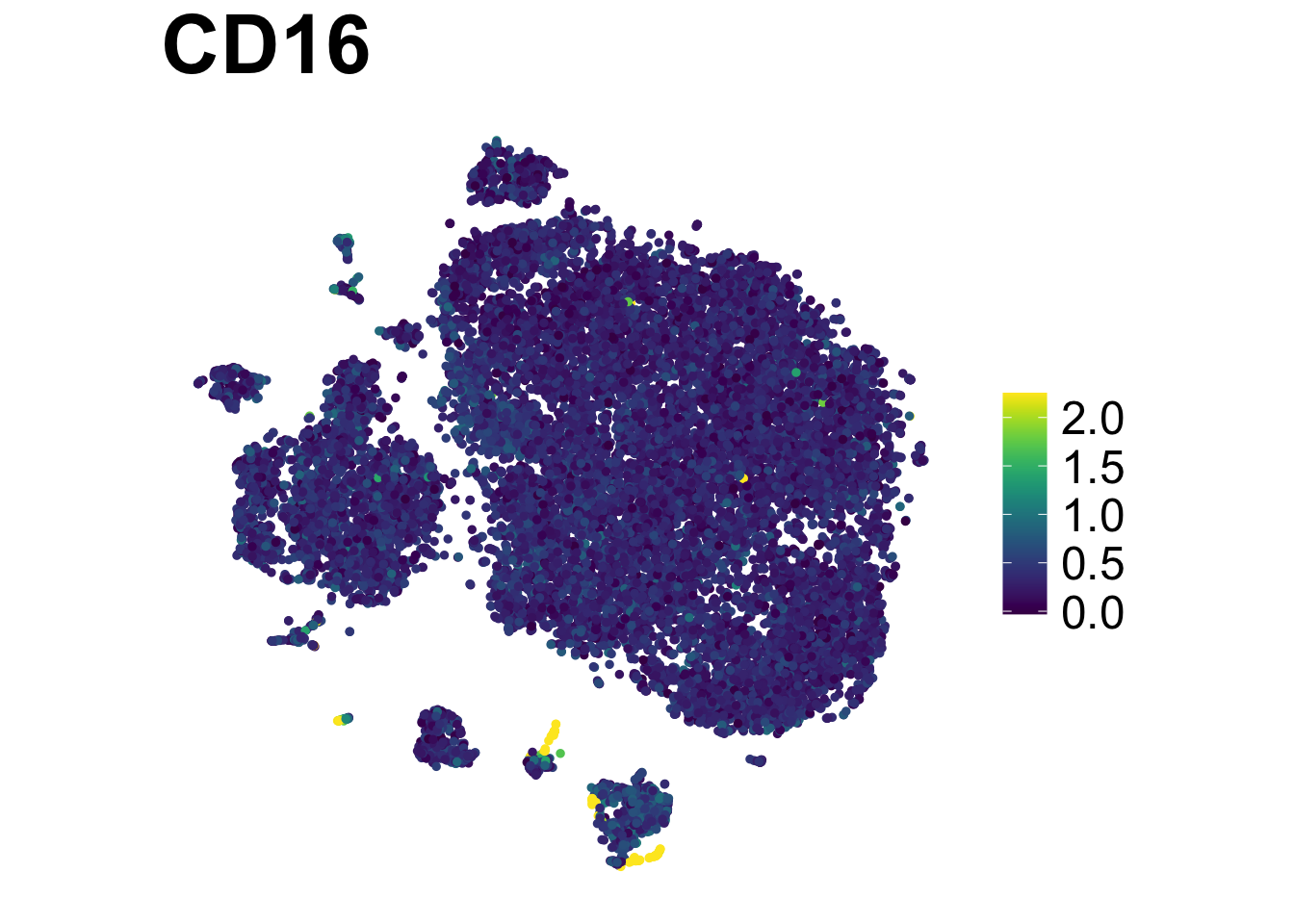
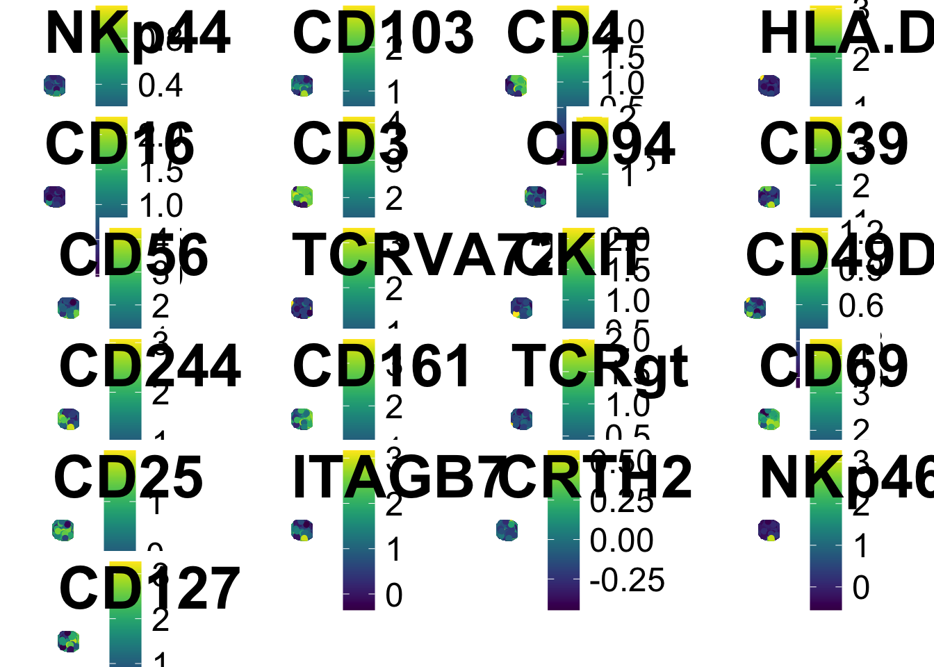
Past versions of unnamed-chunk-33-1.png

Version	Author	Date
2c16dc0	DrThomasOneil	2025-04-28
ec75f7d	DrThomasOneil	2025-04-26

And we can make the heatmap you’re used to seeing and save them.

exp <- do.aggregate(as.data.table(ILC_transf), use.cols = risomMarkers, by = c("flowSOM"))
make.pheatmap(exp, file.name = "plots/Pheatmap_FlowSOM.png", sample.col="flowSOM", plot.cols=risomMarkers)

Spectre has also embedded FlowSOM clustering and dimension reduction tools such as umap in easy codes, such as:

• do.subsample()
• run.flowsom()
• run.umap()
  

Additional Considerations: QC

When looking at the raw data, or in the middle of data processing, you may consider filtering some cell. In the 1-marker plots below, you can see that there are a few extreme values that are displayed and pushing the majority of values squeezed together. e.g. HLA-DR:

ILC_transf %>%
  ggplot(aes(x = HLA.DR))+
  geom_density(linewidth = 0.7, colour = "red", aes(fill = "red"), alpha = 0.5,show.legend = FALSE)+
  ylab("Density")+

# Visualise the values at the top 0.1% and bottom 0.1%.
  geom_vline(xintercept = quantile(ILC_transf$HLA.DR, 0.999), colour = "blue", linewidth = 0.5)+
  geom_vline(xintercept = quantile(ILC_transf$HLA.DR, 0.001), colour = "blue", linewidth = 0.5)+

# We can label the threshold lines: annotate as a text, at the position of the top and bottom 0.01%, and slightly adjust the label position horizontally.
  annotate("text", x = 2, y = 0.5, label = "Top and bottom 0.1%", hjust = -0.1)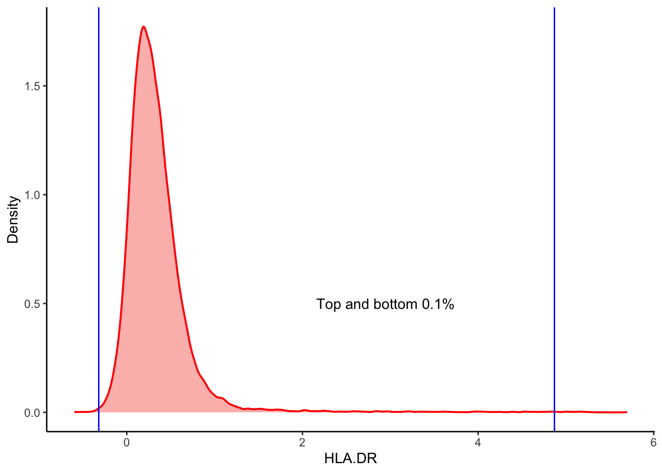 

Past versions of unnamed-chunk-35-1.png

Version	Author	Date
2c16dc0	DrThomasOneil	2025-04-28

View them for all channels.

# Create the empty list
plots_line <- list()

# Create the loop to generate plots.
for (i in 1:25){
  
  # Get the marker names
  Marker <- colnames(ILC_transf)[i]
  
  # Generate the plots and put it into the list
  p <- ILC_transf %>%
  ggplot(aes(x = .data[[Marker]]))+ 
  geom_density(linewidth = 0.7, colour = "red", fill = "red", alpha = 0.3,show.legend = FALSE)+
   xlab(Marker)+
   ylab("Density")+
  
    # Add the newly written lines to visualise the outliers to this loop.
    geom_vline(xintercept = quantile(ILC_transf[[i]], 0.999), colour = "blue", linewidth = 0.5)+
    geom_vline(xintercept = quantile(ILC_transf[[i]], 0.001), colour  = "blue", linewidth = 0.5)
    
  # Put the plots into the list
  plots_line[[length(plots_line)+1]] <- p
}

# Use a grid layout to view the plots
library(ggpubr)
ggpubr::ggarrange(plotlist = plots_line, ncol = 2, nrow = 4)

$`1`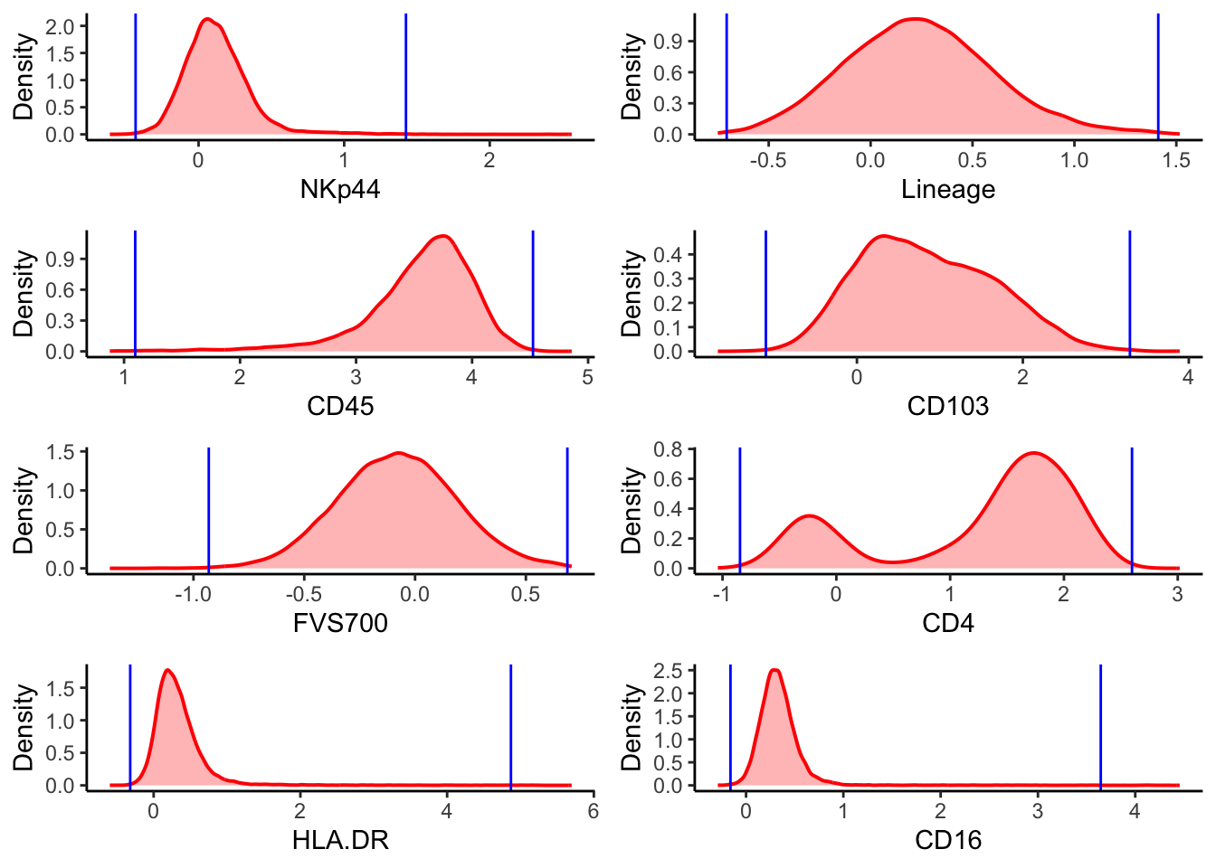

$`2`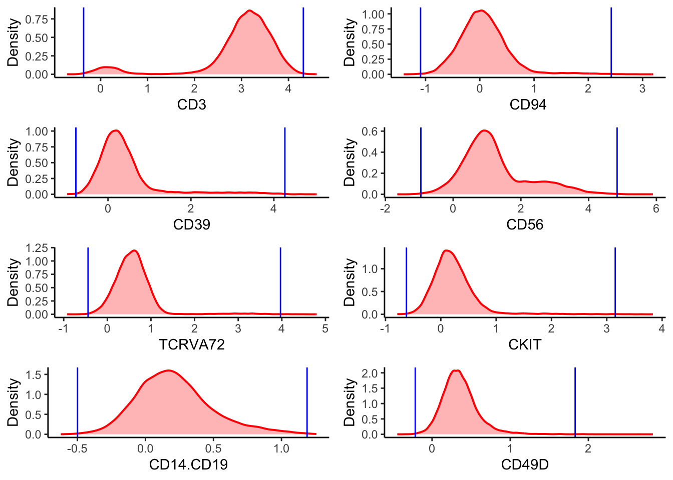

$`3`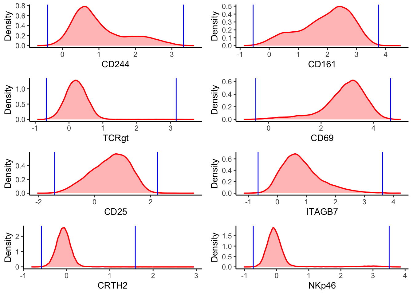

$`4`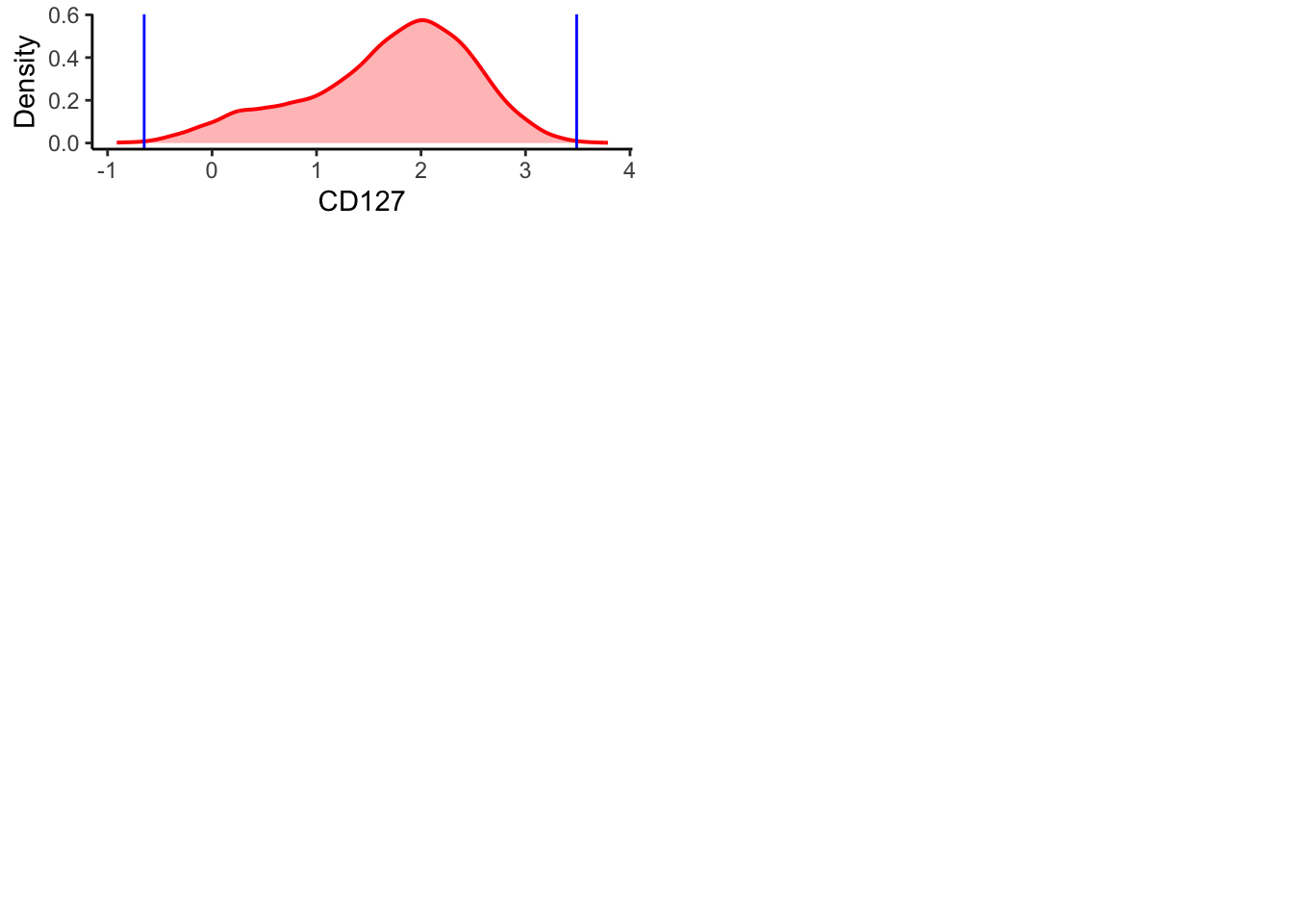

attr(,"class")
[1] "list"      "ggarrange"

To look at this in a more statistical way, you can create a quick data summary of the minimum, maximum, mean, median and the interquartile range.

Expand

summary(ILC_transf)

     NKp44             Lineage              CD45            CD103        
 Min.   :-0.60944   Min.   :-0.74961   Min.   :0.8776   Min.   :-1.6764  
 1st Qu.:-0.02043   1st Qu.:-0.01364   1st Qu.:3.3551   1st Qu.: 0.2275  
 Median : 0.10043   Median : 0.22802   Median :3.6405   Median : 0.7676  
 Mean   : 0.12175   Mean   : 0.23908   Mean   :3.5623   Mean   : 0.8455  
 3rd Qu.: 0.23539   3rd Qu.: 0.47307   3rd Qu.:3.8650   3rd Qu.: 1.4379  
 Max.   : 2.56281   Max.   : 1.51645   Max.   :4.8584   Max.   : 3.8903  
                                                                         
     FVS700              CD4              HLA.DR             CD16        
 Min.   :-1.37739   Min.   :-1.0414   Min.   :-0.5972   Min.   :-0.2901  
 1st Qu.:-0.26103   1st Qu.: 0.7355   1st Qu.: 0.1318   1st Qu.: 0.2128  
 Median :-0.08059   Median : 1.5659   Median : 0.2741   Median : 0.3146  
 Mean   :-0.08100   Mean   : 1.2394   Mean   : 0.3409   Mean   : 0.3452  
 3rd Qu.: 0.09863   3rd Qu.: 1.8856   3rd Qu.: 0.4526   3rd Qu.: 0.4264  
 Max.   : 0.70678   Max.   : 3.0169   Max.   : 5.6978   Max.   : 4.4567  
                                                                         
      CD3              CD94               CD39               CD56        
 Min.   :-0.712   Min.   :-1.40325   Min.   :-0.98439   Min.   :-1.6483  
 1st Qu.: 2.812   1st Qu.:-0.21409   1st Qu.:-0.01198   1st Qu.: 0.5906  
 Median : 3.145   Median : 0.03539   Median : 0.24073   Median : 1.0224  
 Mean   : 2.968   Mean   : 0.06666   Mean   : 0.40428   Mean   : 1.2305  
 3rd Qu.: 3.447   3rd Qu.: 0.29662   3rd Qu.: 0.53662   3rd Qu.: 1.6042  
 Max.   : 4.601   Max.   : 3.19569   Max.   : 5.03303   Max.   : 5.8967  
                                                                         
    TCRVA72             CKIT            CD14.CD19            CD49D        
 Min.   :-0.9207   Min.   :-0.78687   Min.   :-0.62200   Min.   :-0.4446  
 1st Qu.: 0.3260   1st Qu.:-0.01042   1st Qu.: 0.02254   1st Qu.: 0.2099  
 Median : 0.5569   Median : 0.17073   Median : 0.18560   Median : 0.3337  
 Mean   : 0.5825   Mean   : 0.21415   Mean   : 0.21396   Mean   : 0.3559  
 3rd Qu.: 0.7734   3rd Qu.: 0.37904   3rd Qu.: 0.36621   3rd Qu.: 0.4694  
 Max.   : 4.7995   Max.   : 3.83387   Max.   : 1.25671   Max.   : 2.8257  
                                                                          
     CD244             CD161             TCRgt                CD69        
 Min.   :-0.6901   Min.   :-0.8723   Min.   :-0.936193   Min.   :-0.9441  
 1st Qu.: 0.4753   1st Qu.: 1.3699   1st Qu.: 0.006448   1st Qu.: 2.5221  
 Median : 0.8006   Median : 2.0976   Median : 0.210441   Median : 3.0271  
 Mean   : 1.0140   Mean   : 1.9402   Mean   : 0.226867   Mean   : 2.8921  
 3rd Qu.: 1.4233   3rd Qu.: 2.6183   3rd Qu.: 0.422976   3rd Qu.: 3.4394  
 Max.   : 3.6121   Max.   : 4.5151   Max.   : 3.696751   Max.   : 5.0315  
                                                                          
      CD25              ITAGB7            CRTH2              NKp46         
 Min.   :-2.04859   Min.   :-1.1604   Min.   :-0.81326   Min.   :-1.02354  
 1st Qu.: 0.08245   1st Qu.: 0.3493   1st Qu.:-0.17971   1st Qu.:-0.21610  
 Median : 0.62505   Median : 0.7189   Median :-0.07405   Median :-0.07461  
 Mean   : 0.55484   Mean   : 0.8315   Mean   :-0.06856   Mean   : 0.03578  
 3rd Qu.: 1.06689   3rd Qu.: 1.1891   3rd Qu.: 0.03066   3rd Qu.: 0.07985  
 Max.   : 3.55726   Max.   : 4.2459   Max.   : 2.94352   Max.   : 3.86214  
                                                                           
     CD127             FSC.A            FSC.H           FSC.W       
 Min.   :-0.9117   Min.   : 33329   Min.   :15411   Min.   :168801  
 1st Qu.: 1.2209   1st Qu.: 61433   1st Qu.:36705   1st Qu.:238038  
 Median : 1.8260   Median : 72555   Median :45029   Median :244372  
 Mean   : 1.6956   Mean   : 72136   Mean   :45157   Mean   :247282  
 3rd Qu.: 2.2689   3rd Qu.: 82906   3rd Qu.:53280   3rd Qu.:251189  
 Max.   : 3.7882   Max.   :141562   Max.   :95998   Max.   :395580  
                                                                    
     SSC.A           SSC.H           SSC.W             Time        
 Min.   :-2606   Min.   : 3338   Min.   : 90908   Min.   :   1182  
 1st Qu.:15561   1st Qu.:12672   1st Qu.:165542   1st Qu.:1042038  
 Median :19256   Median :15600   Median :172405   Median :2051315  
 Mean   :20342   Mean   :16431   Mean   :174628   Mean   :2077101  
 3rd Qu.:23568   3rd Qu.:18958   3rd Qu.:179231   3rd Qu.:3062559  
 Max.   :97782   Max.   :75316   Max.   :415995   Max.   :4599769  
                                                                   
    subset             flowSOM         fuseSOM            PC1         
 Length:19588       1      :10591   Min.   : 1.000   Min.   :-2.6306  
 Class :character   10     : 2452   1st Qu.: 1.000   1st Qu.:-0.9985  
 Mode  :character   8      : 1681   Median : 1.000   Median :-0.3773  
                    9      : 1404   Mean   : 3.254   Mean   : 0.0000  
                    12     :  867   3rd Qu.: 5.000   3rd Qu.: 0.6658  
                    3      :  755   Max.   :15.000   Max.   : 6.8083  
                    (Other): 1838                                     
      PC2               tSNE1             tSNE2             UMAP1         
 Min.   :-4.08455   Min.   :-43.873   Min.   :-45.939   Min.   :-32.0736  
 1st Qu.:-0.78765   1st Qu.:-12.105   1st Qu.:-11.680   1st Qu.: -2.7945  
 Median :-0.02214   Median :  1.662   Median :  0.542   Median : -0.9637  
 Mean   : 0.00000   Mean   :  0.000   Mean   :  0.000   Mean   :  0.0000  
 3rd Qu.: 0.79000   3rd Qu.: 14.980   3rd Qu.: 12.622   3rd Qu.:  1.8694  
 Max.   : 4.90431   Max.   : 35.063   Max.   : 40.661   Max.   :  9.6477  
                                                                          
     UMAP2       
 Min.   :-5.883  
 1st Qu.:-3.328  
 Median :-1.409  
 Mean   : 0.000  
 3rd Qu.: 1.510  
 Max.   :14.011  
                 

Either being artificial or biological, these might interfere how the computer interprets your data in the downstream clustering and dimension reduction. Sometimes you may decide to investigate how these impact your dataset and where they arise from. But if there are plenty of cells, and the % outliers is super small, you might just want to filter them out.

Filtering by %

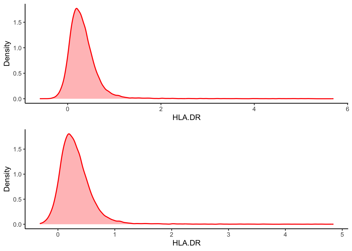
You might want to filter out the top and bottom 0.1% of cells . Note that this approach removes the cells that doesn’t fit within the top and bottom 0.1% of ANY channel, and removes the cell from the entire dataset. So be cautious about the % so you aren’t removing too many cells when they are added up ( we’ll use 0.1% all the way for demonstration purposes).

Expand

# Create an empty list.
outlier_flag <- list()

# Loop through the columns with markers
for (i in 1:25){
  
  # Find the cell values
  value <- ILC_transf[[i]]
  
  # Get the marker names
  Marker <- colnames(ILC_transf)[i]
  
  # Find the thresholds of outliers
  upper <- quantile(value, 0.999, na.rm = TRUE)
  lower <- quantile(value, 0.001, na.rm = TRUE)

  # Flag the outliers as 1, else as 0. And record them into the list.
  flag <- ifelse(value < lower | value > upper, 1, 0)
  outlier_flag[[length(outlier_flag)+1]] <- flag
}
# Turn the flags into a data table object.
outlier_flag <- as.data.table(outlier_flag)
colnames(outlier_flag)<- colnames(ILC_transf)[c(7:31)]
subset <- ILC_transf[rowSums(outlier_flag)==0,]
  
# Calculate the % of cell loss after filtering, then format it as being displayed in less digits, then paste a sentence together.
    paste0("Cell loss: ",format((1-nrow(subset)/nrow(ILC_transf))*100, digits = 3), "%")

[1] "Cell loss: 4.44%"

# View the pre- and post-filtered data side by side, putting them in a grid.
cowplot::plot_grid(
  ILC_transf %>%
  ggplot(aes(x = HLA.DR))+
  geom_density(linewidth = 0.7, colour = "red", fill = "red", alpha = 0.3, show.legend = FALSE)+
  ylab("Density"),

subset %>%
  ggplot(aes(x = HLA.DR))+
  geom_density(linewidth = 0.7, colour = "red", fill = "red", alpha = 0.3, show.legend = FALSE)+
  ylab("Density"),

 # number of column equals 1.
 ncol = 1
)

Past versions of unnamed-chunk-39-1.png

Version	Author	Date
2c16dc0	DrThomasOneil	2025-04-28
ec75f7d	DrThomasOneil	2025-04-26

Filtering by fixed thresholds

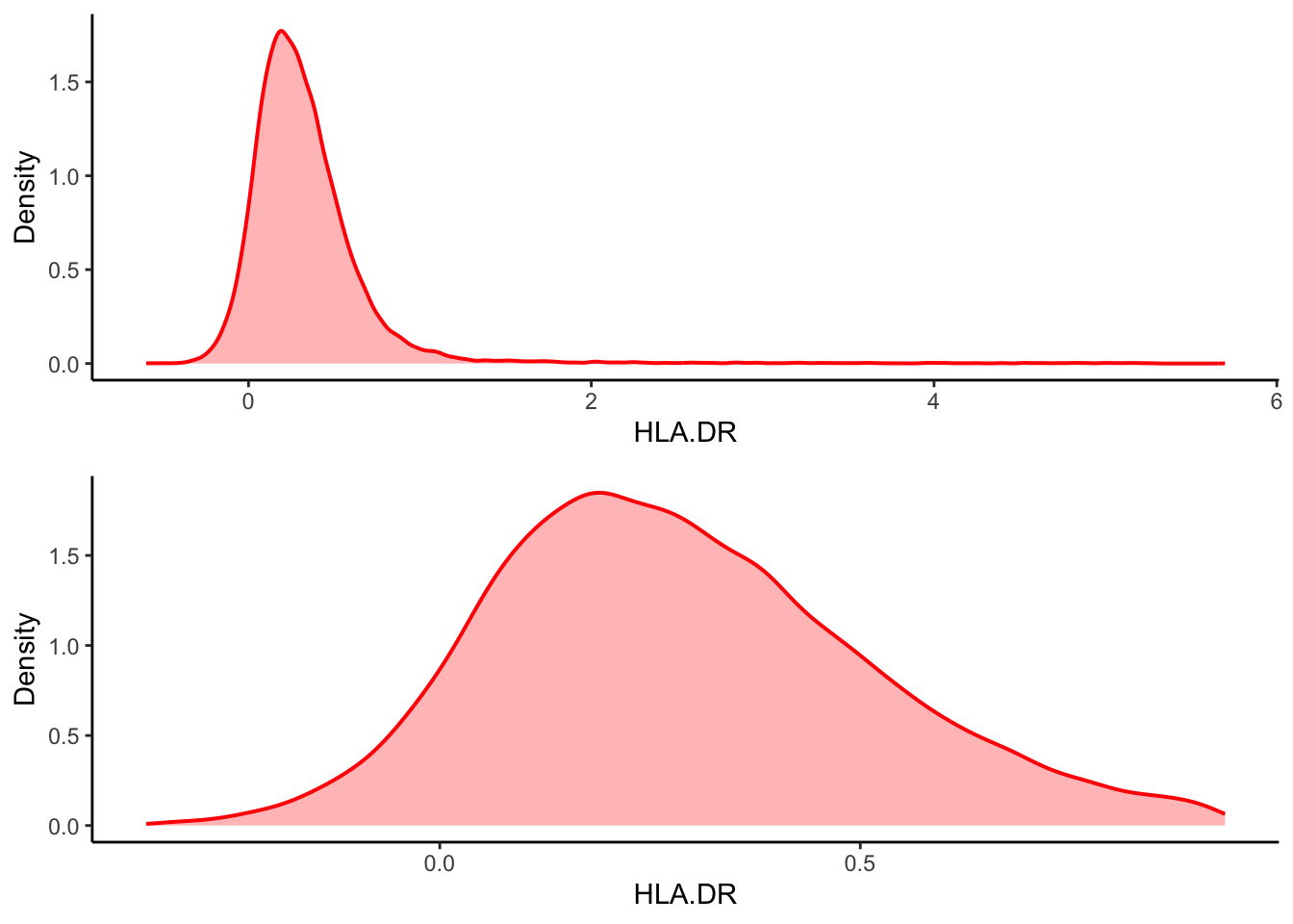
You might want to filter out the data that is outside of certain values per channel. A commonly used standard in data cleaning is calculated based on interquartile ranges (IQR). The thresholds are any data points that are 1.5 times of IQR above the 3rd quartile, or 1.5 times of IQR below the 1st quartile. This will keep the majority of data points, however, it might also remove some true variance in the dataset at extreme ends.

Expand

# Take HLA-DR as an example

# Calculate the interquartile range.
   IQR <- IQR(ILC_transf$HLA.DR)
   Q1 <- quantile(ILC_transf$HLA.DR, 0.25)
   Q3 <- quantile(ILC_transf$HLA.DR, 0.75)
   
# Calculate the upper and lower thresholds
   lowerfence <- Q1 - 1.5*IQR
   upperfence <- Q3 + 1.5*IQR 
 
# Only keep the cells which the HLA-DR value is within the thresholds.   
filt <- ILC_transf[ILC_transf$HLA.DR > lowerfence & ILC_transf$HLA.DR < upperfence, ]

cowplot::plot_grid(
  ILC_transf %>%
  ggplot(aes(x = HLA.DR))+
  geom_density(linewidth = 0.7, colour = "red", fill = "red", alpha = 0.3,show.legend = FALSE)+
  ylab("Density"),
filt %>%
  ggplot(aes(x = HLA.DR))+
  geom_density(linewidth = 0.7, colour = "red", fill = "red", alpha = 0.3,show.legend = FALSE)+
  ylab("Density"),

 # number of column equals 1.
 ncol = 1
)

Past versions of unnamed-chunk-40-1.png

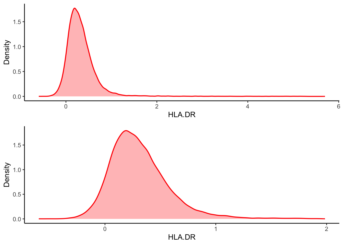
Version	Author	Date
2c16dc0	DrThomasOneil	2025-04-28

rm(Q1,Q3,IQR)

Or, simply just choose an arbitrary threshold.

# Only keep the cells which transformed HLA-DR expression value < 2.
manual <- ILC_transf[ILC_transf$HLA.DR < 2, ]

cowplot::plot_grid(
  ILC_transf %>%
  ggplot(aes(x = HLA.DR))+
  geom_density(linewidth = 0.7, colour = "red", fill = "red", alpha = 0.3,show.legend = FALSE)+
  ylab("Density"),
manual %>%
  ggplot(aes(x = HLA.DR))+
  geom_density(linewidth = 0.7, colour = "red", fill = "red", alpha = 0.3,show.legend = FALSE)+
  ylab("Density"),

 # number of column equals 1.
 ncol = 1
)

Vote on the next workshop!

Session information

sessionInfo()

R version 4.4.0 (2024-04-24)
Platform: aarch64-apple-darwin20
Running under: macOS Sonoma 14.3

Matrix products: default
BLAS:   /Library/Frameworks/R.framework/Versions/4.4-arm64/Resources/lib/libRblas.0.dylib 
LAPACK: /Library/Frameworks/R.framework/Versions/4.4-arm64/Resources/lib/libRlapack.dylib;  LAPACK version 3.12.0

locale:
[1] en_US.UTF-8/en_US.UTF-8/en_US.UTF-8/C/en_US.UTF-8/en_US.UTF-8

time zone: Australia/Sydney
tzcode source: internal

attached base packages:
[1] stats     graphics  grDevices utils     datasets  methods   base     

other attached packages:
 [1] ggpubr_0.6.0         pheatmap_1.0.12      ggpointdensity_0.1.0
 [4] RColorBrewer_1.1-3   ggthemes_5.1.0       colorRamps_2.3.4    
 [7] scales_1.3.0         data.table_1.17.0    Rtsne_0.17          
[10] umap_0.2.10.0        GGally_2.2.1         FlowSOM_2.12.0      
[13] igraph_2.1.4         FuseSOM_1.6.0        Spectre_1.2.0       
[16] cowplot_1.1.3        ggridges_0.5.6       lubridate_1.9.4     
[19] forcats_1.0.0        stringr_1.5.1        dplyr_1.1.4         
[22] purrr_1.0.4          readr_2.1.5          tidyr_1.3.1         
[25] tibble_3.2.1         ggplot2_3.5.1        tidyverse_2.0.0     
[28] workflowr_1.7.1     

loaded via a namespace (and not attached):
  [1] rstudioapi_0.17.1           jsonlite_1.9.1             
  [3] magrittr_2.0.3              DataVisualizations_1.3.3   
  [5] farver_2.1.2                profileModel_0.6.1         
  [7] rmarkdown_2.29              ragg_1.3.3                 
  [9] fs_1.6.5                    zlibbioc_1.50.0            
 [11] vctrs_0.6.5                 askpass_1.2.1              
 [13] rstatix_0.7.2               htmltools_0.5.8.1          
 [15] S4Arrays_1.4.1              broom_1.0.7                
 [17] SparseArray_1.4.8           Formula_1.2-5              
 [19] gridGraphics_0.5-1          sass_0.4.9                 
 [21] bslib_0.9.0                 princurve_2.1.6            
 [23] plyr_1.8.9                  cachem_1.1.0               
 [25] whisker_0.4.1               lifecycle_1.0.4            
 [27] pkgconfig_2.0.3             Matrix_1.7-3               
 [29] R6_2.6.1                    fastmap_1.2.0              
 [31] GenomeInfoDbData_1.2.12     MatrixGenerics_1.16.0      
 [33] digest_0.6.37               ggnewscale_0.5.1           
 [35] colorspace_2.1-1            S4Vectors_0.42.1           
 [37] ps_1.9.0                    rprojroot_2.0.4            
 [39] RSpectra_0.16-2             textshaping_1.0.0          
 [41] GenomicRanges_1.56.2        vegan_2.6-10               
 [43] labeling_0.4.3              cytolib_2.16.0             
 [45] timechange_0.3.0            httr_1.4.7                 
 [47] polyclip_1.10-7             abind_1.4-8                
 [49] coop_0.6-3                  mgcv_1.9-1                 
 [51] compiler_4.4.0              proxy_0.4-27               
 [53] withr_3.0.2                 ConsensusClusterPlus_1.68.0
 [55] backports_1.5.0             carData_3.0-5              
 [57] psych_2.4.12                ggstats_0.9.0              
 [59] ggforce_0.4.2               ggsignif_0.6.4             
 [61] MASS_7.3-65                 openssl_2.3.2              
 [63] DelayedArray_0.30.1         permute_0.9-7              
 [65] tools_4.4.0                 httpuv_1.6.15              
 [67] brglm_0.7.2                 glue_1.8.0                 
 [69] callr_3.7.6                 nlme_3.1-167               
 [71] promises_1.3.2              grid_4.4.0                 
 [73] getPass_0.2-4               cluster_2.1.8.1            
 [75] generics_0.1.3              isoband_0.2.7              
 [77] gtable_0.3.6                tzdb_0.5.0                 
 [79] hms_1.1.3                   utf8_1.2.4                 
 [81] sp_2.2-0                    car_3.1-3                  
 [83] XVector_0.44.0              BiocGenerics_0.50.0        
 [85] pillar_1.10.1               yulab.utils_0.2.0          
 [87] later_1.4.1                 splines_4.4.0              
 [89] flowCore_2.16.0             tweenr_2.0.3               
 [91] lattice_0.22-6              RProtoBufLib_2.16.0        
 [93] tidyselect_1.2.1            knitr_1.50                 
 [95] git2r_0.35.0                gridExtra_2.3              
 [97] IRanges_2.38.1              SummarizedExperiment_1.34.0
 [99] analogue_0.17-7             stats4_4.4.0               
[101] xfun_0.51                   Biobase_2.64.0             
[103] matrixStats_1.5.0           stringi_1.8.4              
[105] UCSC.utils_1.0.0            yaml_2.3.10                
[107] evaluate_1.0.3              ggplotify_0.1.2            
[109] cli_3.6.4                   systemfonts_1.2.1          
[111] reticulate_1.41.0.1         munsell_0.5.1              
[113] processx_3.8.6              jquerylib_0.1.4            
[115] Rcpp_1.0.14                 GenomeInfoDb_1.40.1        
[117] png_0.1-8                   FCPS_1.3.4                 
[119] fastcluster_1.2.6           XML_3.99-0.18              
[121] parallel_4.4.0              mclust_6.1.1               
[123] viridisLite_0.4.2           crayon_1.5.3               
[125] rlang_1.1.6                 mnormt_2.1.1               

Digital Research Skills Network
Contact us