Molecular Cartography - Seurat analysis

workflowr

• Summary
• Checks
• Past versions

Last updated: 2024-03-21

Checks: 7 0

Knit directory: mi_spatialomics/

This reproducible R Markdown analysis was created with workflowr (version 1.7.1). The Checks tab describes the reproducibility checks that were applied when the results were created. The Past versions tab lists the development history.

---

R Markdown file: up-to-date

Great! Since the R Markdown file has been committed to the Git repository, you know the exact version of the code that produced these results.

Environment: empty

Great job! The global environment was empty. Objects defined in the global environment can affect the analysis in your R Markdown file in unknown ways. For reproduciblity it’s best to always run the code in an empty environment.

Seed: set.seed(20230612)

The command set.seed(20230612) was run prior to running the code in the R Markdown file. Setting a seed ensures that any results that rely on randomness, e.g. subsampling or permutations, are reproducible.

Session information: recorded

Great job! Recording the operating system, R version, and package versions is critical for reproducibility.

Cache: none

Nice! There were no cached chunks for this analysis, so you can be confident that you successfully produced the results during this run.

File paths: relative

Great job! Using relative paths to the files within your workflowr project makes it easier to run your code on other machines.

Repository version: e6213a5

Great! You are using Git for version control. Tracking code development and connecting the code version to the results is critical for reproducibility.

The results in this page were generated with repository version e6213a5. See the Past versions tab to see a history of the changes made to the R Markdown and HTML files.

Note that you need to be careful to ensure that all relevant files for the analysis have been committed to Git prior to generating the results (you can use wflow_publish or wflow_git_commit). workflowr only checks the R Markdown file, but you know if there are other scripts or data files that it depends on. Below is the status of the Git repository when the results were generated:

Ignored files:
    Ignored:    .DS_Store
    Ignored:    .Rproj.user/
    Ignored:    analysis/.DS_Store
    Ignored:    analysis/deprecated/.DS_Store
    Ignored:    analysis/molecular_cartography_python/.DS_Store
    Ignored:    analysis/seqIF_python/.DS_Store
    Ignored:    analysis/seqIF_python/pixie/.DS_Store
    Ignored:    analysis/seqIF_python/pixie/cell_clustering/
    Ignored:    annotations/.DS_Store
    Ignored:    annotations/SeqIF/.DS_Store
    Ignored:    annotations/molkart/.DS_Store
    Ignored:    annotations/molkart/Figure1_regions/.DS_Store
    Ignored:    annotations/molkart/Supplementary_Figure4_regions/.DS_Store
    Ignored:    data/.DS_Store
    Ignored:    data/140623.calcagno_et_al.seurat_object.rds
    Ignored:    data/Calcagno2022_int_logNorm_annot.h5Seurat
    Ignored:    data/IC_03_IF_CCR2_CD68 cell numbers.xlsx
    Ignored:    data/Traditional_IF_absolute_cell_counts.csv
    Ignored:    data/Traditional_IF_relative_cell_counts.csv
    Ignored:    data/pixie.cell_table_size_normalized_cell_labels.csv
    Ignored:    data/results_cts_100.sqm
    Ignored:    data/seqIF_regions_annotations/
    Ignored:    data/seurat/
    Ignored:    output/.DS_Store
    Ignored:    output/mol_cart.harmony_object.h5Seurat
    Ignored:    output/molkart/
    Ignored:    output/proteomics/
    Ignored:    output/results_cts.lowres.125.sqm
    Ignored:    output/seqIF/
    Ignored:    pipeline_configs/.DS_Store
    Ignored:    plots/
    Ignored:    references/.DS_Store
    Ignored:    renv/.DS_Store
    Ignored:    renv/library/
    Ignored:    renv/staging/

Untracked files:
    Untracked:  analysis/deprecated/figures.supplementary_figureX.Rmd
    Untracked:  analysis/deprecated/figures.supplementary_figure_X.MistyR.Rmd

Unstaged changes:
    Deleted:    analysis/figures.supplementary_figureX.Rmd
    Deleted:    analysis/figures.supplementary_figure_X.MistyR.Rmd
    Deleted:    analysis/figures.supplementary_figure_X.proteomics_qc.Rmd
    Deleted:    figures/Figure_5.eps
    Deleted:    figures/Figure_5.pdf
    Deleted:    figures/Figure_5.png
    Deleted:    figures/Figure_5.svg
    Deleted:    figures/Supplementary_Figure_1_Molecular_Cartography_ROIs.png
    Deleted:    figures/Supplementary_figure_5.segmentation_metrics.poster.eps
    Modified:   figures/Supplementary_figure_X.proteomics.eps
    Modified:   figures/Supplementary_figure_X.proteomics.png
    Modified:   results_cts.lowres.125.sqm

Note that any generated files, e.g. HTML, png, CSS, etc., are not included in this status report because it is ok for generated content to have uncommitted changes.

---

These are the previous versions of the repository in which changes were made to the R Markdown (analysis/molkart.seurat_analysis.Rmd) and HTML (docs/molkart.seurat_analysis.html) files. If you’ve configured a remote Git repository (see ?wflow_git_remote), click on the hyperlinks in the table below to view the files as they were in that past version.

File	Version	Author	Date	Message
Rmd	56559c7	FloWuenne	2024-03-21	Cleaned up repository.
Rmd	b06dcd3	FloWuenne	2024-02-25	Updated Figure 1,4 and S4 and 5 code.
Rmd	af64c40	FloWuenne	2024-01-30	Updated analysis for Figure 1 and 2.
Rmd	86e53f0	FloWuenne	2024-01-22	Finalized new Figure 1 plots.
Rmd	82f107f	FloWuenne	2024-01-21	Updates to Molkart analysis.
Rmd	f4d5c82	FloWuenne	2024-01-15	Latest update to Seurat analysis with reprocessed data.
Rmd	2d9b909	FloWuenne	2024-01-09	Pushing latest changes. Updating molkart data.
Rmd	60d835c	FloWuenne	2023-12-06	Updated renv packages.

---

library(Seurat)

Loading required package: SeuratObject

Loading required package: sp

'SeuratObject' was built with package 'Matrix' 1.6.3 but the current
version is 1.6.5; it is recomended that you reinstall 'SeuratObject' as
the ABI for 'Matrix' may have changed

Attaching package: 'SeuratObject'

The following object is masked from 'package:base':

    intersect

library(SeuratData)
library(SeuratDisk)

Registered S3 method overwritten by 'SeuratDisk':
  method            from  
  as.sparse.H5Group Seurat

library(data.table)
library(harmony)

Loading required package: Rcpp

library(here)

here() starts at /Users/florian_wuennemann/1_Projects/MI_project/mi_spatialomics

library(Nebulosa)

Loading required package: ggplot2

Loading required package: patchwork

library(tidyverse)

── Attaching core tidyverse packages ──────────────────────── tidyverse 2.0.0 ──
✔ dplyr     1.1.4     ✔ readr     2.1.5
✔ forcats   1.0.0     ✔ stringr   1.5.1
✔ lubridate 1.9.3     ✔ tibble    3.2.1
✔ purrr     1.0.2     ✔ tidyr     1.3.0

── Conflicts ────────────────────────────────────────── tidyverse_conflicts() ──
✖ dplyr::between()     masks data.table::between()
✖ dplyr::filter()      masks stats::filter()
✖ dplyr::first()       masks data.table::first()
✖ lubridate::hour()    masks data.table::hour()
✖ lubridate::isoweek() masks data.table::isoweek()
✖ dplyr::lag()         masks stats::lag()
✖ dplyr::last()        masks data.table::last()
✖ lubridate::mday()    masks data.table::mday()
✖ lubridate::minute()  masks data.table::minute()
✖ lubridate::month()   masks data.table::month()
✖ lubridate::quarter() masks data.table::quarter()
✖ lubridate::second()  masks data.table::second()
✖ purrr::transpose()   masks data.table::transpose()
✖ lubridate::wday()    masks data.table::wday()
✖ lubridate::week()    masks data.table::week()
✖ lubridate::yday()    masks data.table::yday()
✖ lubridate::year()    masks data.table::year()
ℹ Use the conflicted package (<http://conflicted.r-lib.org/>) to force all conflicts to become errors

library(GGally)

Registered S3 method overwritten by 'GGally':
  method from   
  +.gg   ggplot2

library(Matrix)

Attaching package: 'Matrix'

The following objects are masked from 'package:tidyr':

    expand, pack, unpack

library(sf)

Linking to GEOS 3.11.0, GDAL 3.5.3, PROJ 9.1.0; sf_use_s2() is TRUE

library(sfheaders)
library(viridis)

Loading required package: viridisLite

source("./code/functions.R")

Attaching package: 'cowplot'

The following object is masked from 'package:lubridate':

    stamp

The following object is masked from 'package:patchwork':

    align_plots

Introduction

In this analysis, we will process the single-cell quantification from nf-Molkart. These tables are basically the output from the regionprops command from scikit and contain properties from the segmentation masks, as well as the count of RNA molecules per gene. We will parse these tables to extract the transcript counts, put these in the expression matrix slots from Seurat and extract the metadata for samples and segmentation masks and put these into the metadata slot of Seurat objects.

Read data

Process mcquant tables to seurat object

First, we read the samples, create Seurat objects for them and then merge the Seurat objects.

Merging seurat objects

final_samples <- c("sample_control_r1_s1","sample_control_r2_s1",
                   "sample_4h_r1_s1","sample_4h_r2_s2",
                   "sample_2d_r1_s1","sample_2d_r2_s1",
                   "sample_4d_r1_s1","sample_4d_r2_s1")

seurat_objects <- list()
norm_list <- list()

## SCTransform based clustering across all samples
sample_dir <- "../data/nf-core_molkart/spot2cell"
seurat_list <- list()
segmethod_samples <- list.files(sample_dir)
for(sample in segmethod_samples){
    sample_ID <- strsplit(sample,"\\.")[[1]][1]
    sample_ID <- strsplit(sample_ID,split="_")[[1]][-1]
    sample_ID <- paste(sample_ID[1:length(sample_ID) -1],collapse = "_")
    if(endsWith(sample,"_cellpose.csv") & sample_ID %in% final_samples){
      print(sample_ID)
      sample_quant <- fread(paste(sample_dir,sample,sep="/"))
      seurat_object <- create_seurat_sctransform_mcquant(sample_quant,sample_ID)
      # norm_list[[sample_ID]] <- seurat_object@assays$RNA@layers$counts / seurat_object@meta.data$Area
      seurat_list[[sample_ID]] <- seurat_object
  }
}

[1] "sample_2d_r1_s1"

Warning: Data is of class matrix. Coercing to dgCMatrix.

[1] "sample_2d_r2_s1"

Warning: Data is of class matrix. Coercing to dgCMatrix.

[1] "sample_4d_r1_s1"

Warning: Data is of class matrix. Coercing to dgCMatrix.

[1] "sample_4d_r2_s1"

Warning: Data is of class matrix. Coercing to dgCMatrix.

[1] "sample_4h_r1_s1"

Warning: Data is of class matrix. Coercing to dgCMatrix.

[1] "sample_4h_r2_s2"

Warning: Data is of class matrix. Coercing to dgCMatrix.

[1] "sample_control_r1_s1"

Warning: Data is of class matrix. Coercing to dgCMatrix.

[1] "sample_control_r2_s1"

Warning: Data is of class matrix. Coercing to dgCMatrix.

resolve_object <- merge(seurat_list[[1]], y = c(seurat_list[-1]), 
                        project = "molkart_MI", merge.data = TRUE)
resolve_object <- JoinLayers(resolve_object)

Process data

Now, we will filter cells based on some general quality control parameters like a minimum number of RNA molecules detected and also remove some weirdly shaped cell masks.

Plot distribution of transcript counts and mask properties

## Set order of timepoints
resolve_object@meta.data$timepoint <- factor(resolve_object@meta.data$timepoint,
                               levels = c("control","4h","2d","4d"))


## Show distribution of QC measures before filtering outliers
VlnPlot(resolve_object, features = c("nCount_RNA","nFeature_RNA","Area","Eccentricity","Solidity"),
        group.by = "timepoint", pt.size = 0, cols = time_palette)

Warning: Default search for "data" layer in "RNA" assay yielded no results;
utilizing "counts" layer instead.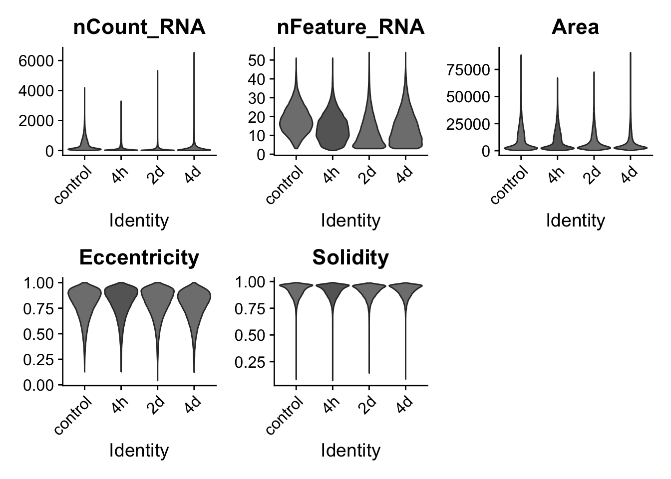

prefiltered_cells <- nrow(resolve_object@meta.data)
print(paste(prefiltered_cells,"cells before filtering"))

[1] "83606 cells before filtering"

Filter outlier cells

## Before filtering cells, let's see if there are any specific outliers
meta_props <- resolve_object@meta.data %>%
  select(Area,MajorAxisLength,MinorAxisLength,Eccentricity,Solidity,Extent,nCount_RNA,timepoint)

ggpairs(meta_props, 
        mapping = aes(color = timepoint),
        columns = c("Area", "Solidity", "Extent","nCount_RNA"))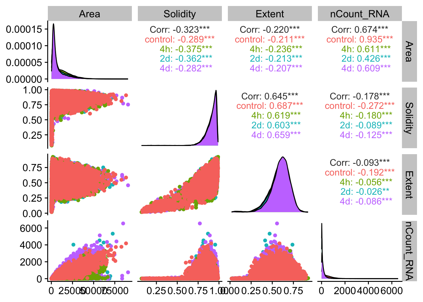

resolve_object <- subset(resolve_object, 
                         subset = 
                           nCount_RNA <= 4000 & 
                           nCount_RNA >= 20 &
                           Extent > 0.25 &
                           Solidity > 0.75)

## How many cells are left after filtering?
post_filter_cells <- nrow(resolve_object@meta.data)

## Let's check the same correlations after filtering
meta_props <- resolve_object@meta.data %>%
  select(Area,MajorAxisLength,MinorAxisLength,Eccentricity,Solidity,Extent,nCount_RNA,timepoint)

ggpairs(meta_props, 
        mapping = aes(color = timepoint),
        columns = c("Area", "Solidity", "Extent","nCount_RNA"))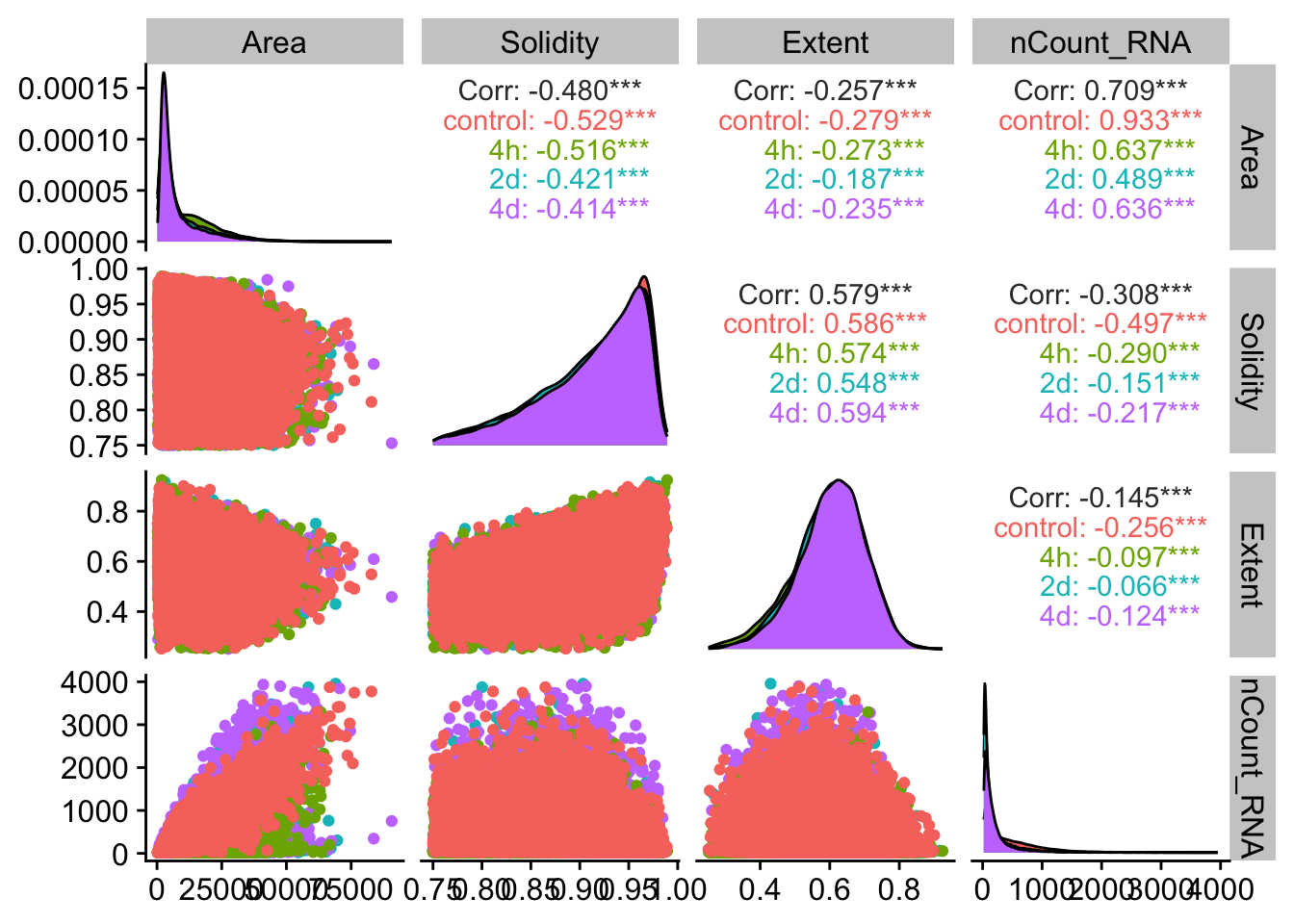

## Show distribution of QC measures after filtering outliers
VlnPlot(resolve_object, features = c("nCount_RNA","nFeature_RNA","Area","Eccentricity","Solidity"),
        group.by = "timepoint", pt.size = 0, cols = time_palette)

Warning: Default search for "data" layer in "RNA" assay yielded no results;
utilizing "counts" layer instead.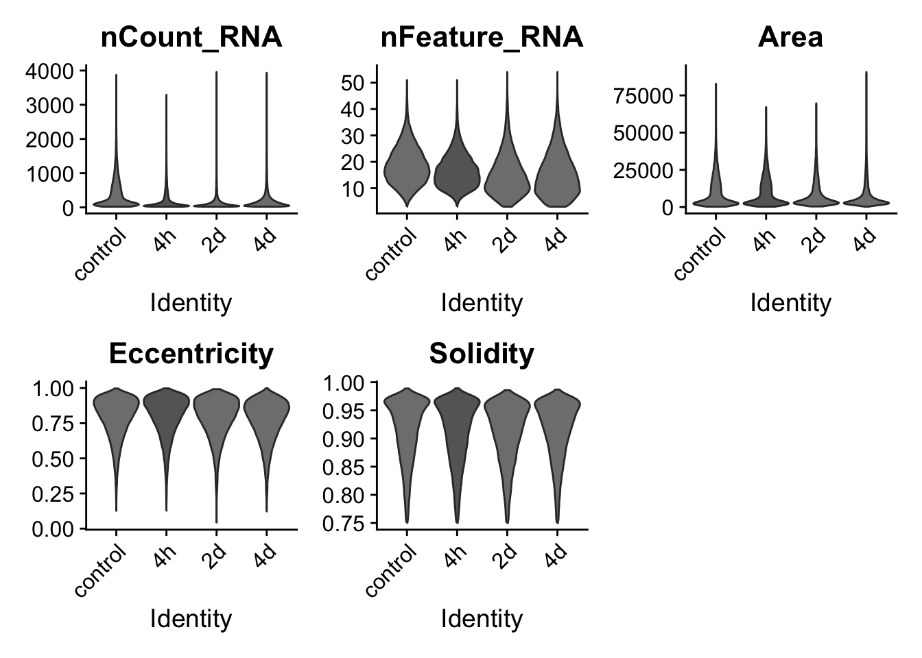

Integrate samples using SCTransform and Harmony

Now we will integrate the different samples using the harmony method within Seurat.

resolve_object[["RNA"]] <- split(resolve_object[["RNA"]], f = resolve_object$timepoint)

## Normalize and scale data using sctransform v2
resolve_object <- SCTransform(resolve_object, 
                              assay = "RNA")

Running SCTransform on assay: RNA

Running SCTransform on layer: counts.2d

vst.flavor='v2' set. Using model with fixed slope and excluding poisson genes.

Variance stabilizing transformation of count matrix of size 93 by 9183

Model formula is y ~ log_umi

Get Negative Binomial regression parameters per gene

Using 93 genes, 5000 cells

Second step: Get residuals using fitted parameters for 93 genes

Computing corrected count matrix for 93 genes

Calculating gene attributes

Wall clock passed: Time difference of 0.8328509 secs

Determine variable features

Centering data matrix

Getting residuals for block 1(of 2) for 2d dataset

Getting residuals for block 2(of 2) for 2d dataset

Centering data matrix

Finished calculating residuals for 2d

Running SCTransform on layer: counts.4d

vst.flavor='v2' set. Using model with fixed slope and excluding poisson genes.

Variance stabilizing transformation of count matrix of size 99 by 19015

Model formula is y ~ log_umi

Get Negative Binomial regression parameters per gene

Using 94 genes, 5000 cells

Second step: Get residuals using fitted parameters for 99 genes

Computing corrected count matrix for 99 genes

Calculating gene attributes

Wall clock passed: Time difference of 0.985574 secs

Determine variable features

Centering data matrix

Getting residuals for block 1(of 4) for 4d dataset

Getting residuals for block 2(of 4) for 4d dataset

Getting residuals for block 3(of 4) for 4d dataset

Getting residuals for block 4(of 4) for 4d dataset

Centering data matrix

Finished calculating residuals for 4d

Running SCTransform on layer: counts.4h

vst.flavor='v2' set. Using model with fixed slope and excluding poisson genes.

Variance stabilizing transformation of count matrix of size 95 by 20155

Model formula is y ~ log_umi

Get Negative Binomial regression parameters per gene

Using 94 genes, 5000 cells

Second step: Get residuals using fitted parameters for 95 genes

Computing corrected count matrix for 95 genes

Calculating gene attributes

Wall clock passed: Time difference of 0.6392071 secs

Determine variable features

Centering data matrix

Getting residuals for block 1(of 5) for 4h dataset

Getting residuals for block 2(of 5) for 4h dataset

Getting residuals for block 3(of 5) for 4h dataset

Getting residuals for block 4(of 5) for 4h dataset

Getting residuals for block 5(of 5) for 4h dataset

Centering data matrix

Finished calculating residuals for 4h

Running SCTransform on layer: counts.control

vst.flavor='v2' set. Using model with fixed slope and excluding poisson genes.

Variance stabilizing transformation of count matrix of size 93 by 20675

Model formula is y ~ log_umi

Get Negative Binomial regression parameters per gene

Using 89 genes, 5000 cells

Found 2 outliers - those will be ignored in fitting/regularization step

Second step: Get residuals using fitted parameters for 93 genes

Computing corrected count matrix for 93 genes

Calculating gene attributes

Wall clock passed: Time difference of 0.636632 secs

Determine variable features

Centering data matrix

Getting residuals for block 1(of 5) for control dataset

Getting residuals for block 2(of 5) for control dataset

Getting residuals for block 3(of 5) for control dataset

Getting residuals for block 4(of 5) for control dataset

Getting residuals for block 5(of 5) for control dataset

Centering data matrix

Finished calculating residuals for control

Set default assay to SCT

# Perform PCA
npcs_to_use <- 30
resolve_object <- RunPCA(resolve_object, npcs = npcs_to_use, verbose = FALSE, approx=FALSE)
ElbowPlot(resolve_object, ndims = npcs_to_use)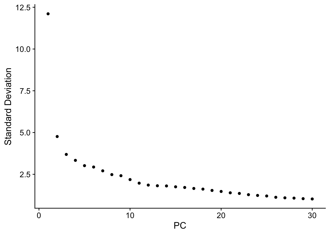

harmony_object <- IntegrateLayers(
  object = resolve_object, method = HarmonyIntegration,
  orig.reduction = "pca", new.reduction = "harmony",
  assay = "SCT", verbose = FALSE
)

Warning: HarmonyMatrix is deprecated and will be removed in the future from the
API in the future

Warning: Warning: The parameters do_pca and npcs are deprecated. They will be ignored for this function call and please remove parameters do_pca and npcs and pass to harmony cell_embeddings directly.
This warning is displayed once per session.

Warning: Warning: The parameter tau is deprecated. It will be ignored for this function call and please remove parameter tau in future function calls. Advanced users can set value of parameter tau by using parameter .options and function harmony_options().
This warning is displayed once per session.

Warning: Warning: The parameter block.size is deprecated. It will be ignored for this function call and please remove parameter block.size in future function calls. Advanced users can set value of parameter block.size by using parameter .options and function harmony_options().
This warning is displayed once per session.

Warning: Warning: The parameter max.iter.harmony is replaced with parameter max_iter. It will be ignored for this function call and please use parameter max_iter in future function calls.
This warning is displayed once per session.

Warning: Warning: The parameter max.iter.cluster is deprecated. It will be ignored for this function call and please remove parameter max.iter.cluster in future function calls. Advanced users can set value of parameter max.iter.cluster by using parameter .options and function harmony_options().
This warning is displayed once per session.

Warning: Warning: The parameter epsilon.cluster is deprecated. It will be ignored for this function call and please remove parameter epsilon.cluster in future function calls. Advanced users can set value of parameter epsilon.cluster by using parameter .options and function harmony_options().
This warning is displayed once per session.

Warning: Warning: The parameter epsilon.harmony is deprecated. It will be ignored for this function call and please remove parameter epsilon.harmony in future function calls. If users want to control if harmony would stop early or not, use parameter early_stop. Advanced users can set value of parameter epsilon.harmony by using parameter .options and function harmony_options().
This warning is displayed once per session.

Warning: Quick-TRANSfer stage steps exceeded maximum (= 3451400)

harmony_object <- FindNeighbors(harmony_object, reduction = "harmony", dims = 1:npcs_to_use)

Computing nearest neighbor graph

Computing SNN

harmony_object <- FindClusters(harmony_object, resolution = 0.4, cluster.name = "harmony_clusters")

Modularity Optimizer version 1.3.0 by Ludo Waltman and Nees Jan van Eck

Number of nodes: 69028
Number of edges: 2495751

Running Louvain algorithm...
Maximum modularity in 10 random starts: 0.9460
Number of communities: 24
Elapsed time: 15 seconds

harmony_object <- RunUMAP(harmony_object, reduction = "harmony", dims = 1:npcs_to_use, reduction.name = "umap")

Warning: The default method for RunUMAP has changed from calling Python UMAP via reticulate to the R-native UWOT using the cosine metric
To use Python UMAP via reticulate, set umap.method to 'umap-learn' and metric to 'correlation'
This message will be shown once per session

21:19:09 UMAP embedding parameters a = 0.9922 b = 1.112

Found more than one class "dist" in cache; using the first, from namespace 'spam'

Also defined by 'BiocGenerics'

21:19:09 Read 69028 rows and found 30 numeric columns

21:19:09 Using Annoy for neighbor search, n_neighbors = 30

Found more than one class "dist" in cache; using the first, from namespace 'spam'

Also defined by 'BiocGenerics'

21:19:09 Building Annoy index with metric = cosine, n_trees = 50

0%   10   20   30   40   50   60   70   80   90   100%

[----|----|----|----|----|----|----|----|----|----|

**************************************************|
21:19:16 Writing NN index file to temp file /var/folders/ph/m6mhj3s541799cykzbp3dx0m0000gn/T//RtmpgOWfRi/file1304382ad87d
21:19:17 Searching Annoy index using 1 thread, search_k = 3000
21:19:36 Annoy recall = 98.6%
21:19:36 Commencing smooth kNN distance calibration using 1 thread with target n_neighbors = 30
21:19:37 Initializing from normalized Laplacian + noise (using RSpectra)
21:19:39 Commencing optimization for 200 epochs, with 3233778 positive edges
21:20:04 Optimization finished

p1 <- plot_density(harmony_object, features= c("Npr3"), size = 0.5)
p2 <- DimPlot(harmony_object, reduction = "umap", label = TRUE, repel = TRUE,raster=FALSE)
p1+p2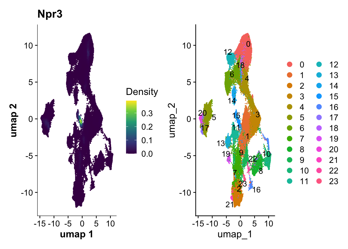

Plot Harmony integration results

## Plot UMAP with cells labeled by sampled time point and by cluster assigned using nearest-neighbor analysis
p1 <- DimPlot(harmony_object, reduction = "umap", group.by = "timepoint",raster=FALSE, 
              cols = time_palette, alpha = 0.5)
p2 <- DimPlot(harmony_object, reduction = "umap", label = TRUE, repel = TRUE,raster=FALSE)
p1+p2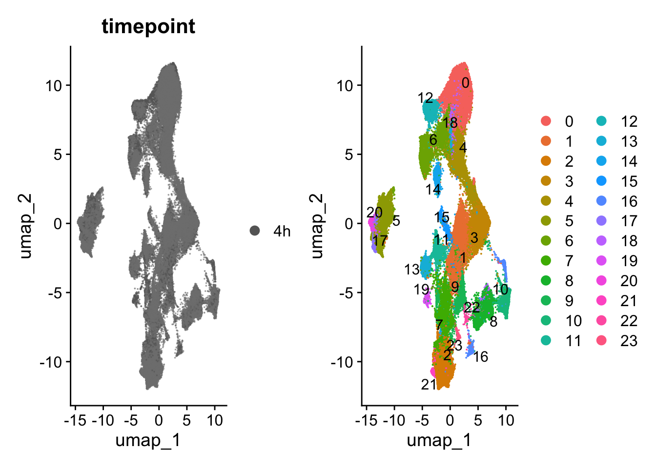

## Plot UMAP next to a barplot
meta_time <- harmony_object@meta.data %>%
  group_by(seurat_clusters, timepoint) %>%
  tally() %>%
  mutate("frac" = n / sum(n))

time_bar <- ggplot(meta_time,aes(seurat_clusters,frac, fill = timepoint)) +
  geom_bar(stat = "identity", position = "stack") +
  coord_flip() +
  scale_fill_manual(values = time_palette)

combined_time_plot <- p2 + time_bar & 
  theme(plot.background = element_rect(fill = 'white'),
        panel.background = element_rect(fill = 'white'))

save_plot(combined_time_plot,
          file = "./plots/molkart.umap_time.png",
          base_height = 10)

## Plot Nebulosa plots for QC measures to highlight cell clusters with high number of transcripts
plot_density(harmony_object, features= c("Area","nCount_RNA","Solidity","Extent"))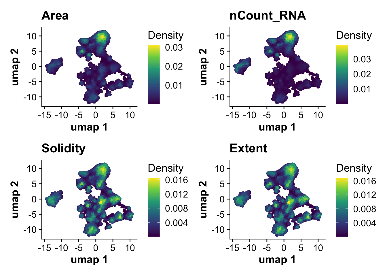

## Plot the number of cells per cluster and color by cluster ID
cell_numbers <- harmony_object@meta.data %>%
  group_by(seurat_clusters) %>%
  tally()

ggplot(cell_numbers,aes(seurat_clusters,n)) +
  geom_bar(stat = "identity",aes(fill = seurat_clusters)) +
  theme(legend.position = "None")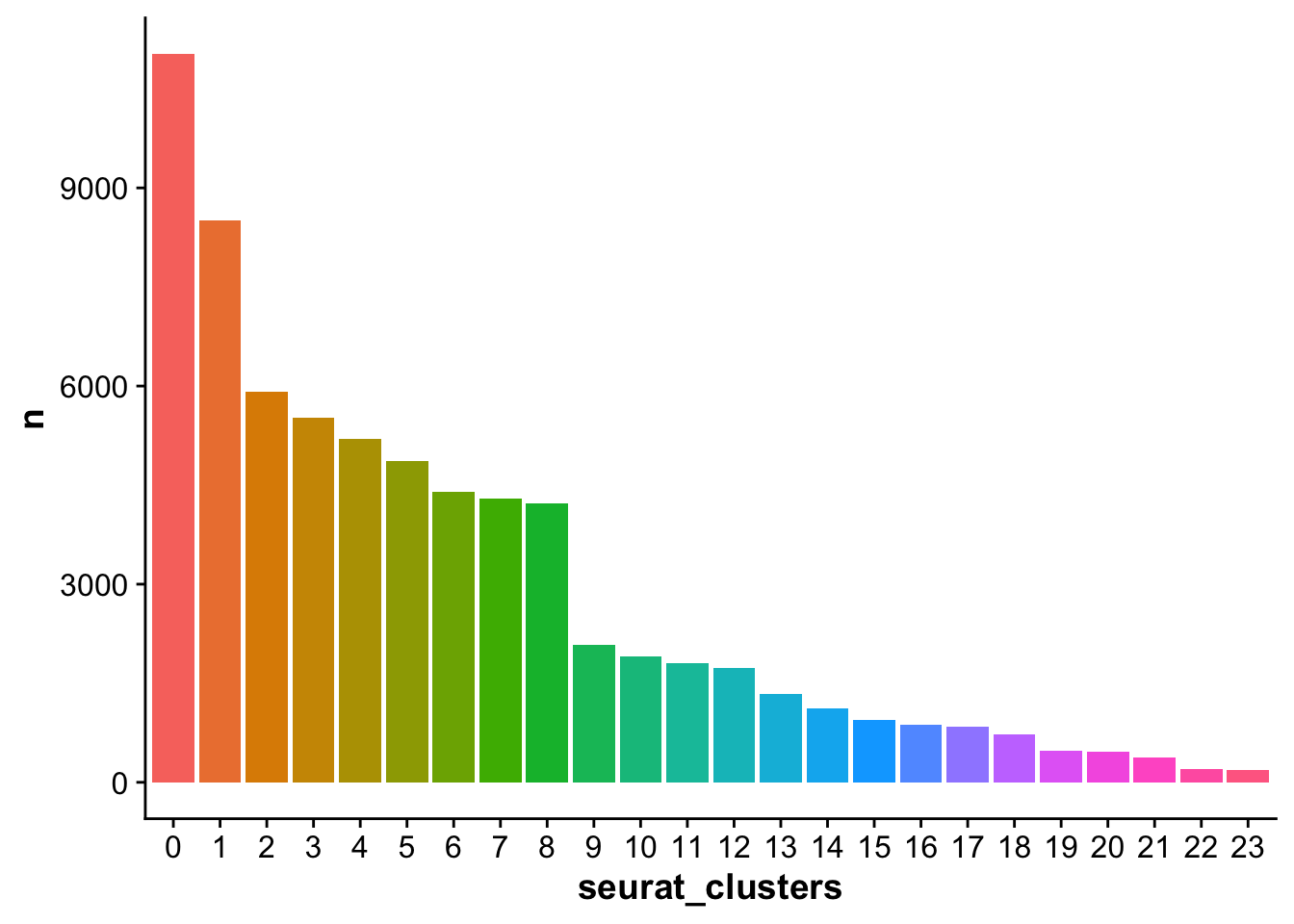

Identify marker genes for cell clusters

harmony_object <- PrepSCTFindMarkers(harmony_object, assay = "SCT", verbose = TRUE)

Found 4 SCT models. Recorrecting SCT counts using minimum median counts: 78

harmony_markers <- FindAllMarkers(harmony_object, logfc.threshold = 0.5, only.pos = TRUE)

Calculating cluster 0

Calculating cluster 1

Calculating cluster 2

Calculating cluster 3

Calculating cluster 4

Calculating cluster 5

Calculating cluster 6

Calculating cluster 7

Calculating cluster 8

Calculating cluster 9

Calculating cluster 10

Calculating cluster 11

Calculating cluster 12

Calculating cluster 13

Calculating cluster 14

Calculating cluster 15

Calculating cluster 16

Calculating cluster 17

Calculating cluster 18

Calculating cluster 19

Calculating cluster 20

Calculating cluster 21

Calculating cluster 22

Calculating cluster 23

## Write marker table to file
write.table(harmony_markers,
            file = "./output/molkart/molkart.cell_type_markers.csv",
            sep = ",",
            row.names = TRUE,
            col.names = TRUE,
            quote = FALSE)

Transfer labels from snRNA-seq (Calcagno et al. 2020)

To get some labels for cell types from a publicly available dataset, we will transfer labels from an snRNA-seq dataset generated by Calcagno et al. 2020 in Nature cardiovascular research.

calcagno_et_al <- LoadH5Seurat("../public_data/Calcagno_et_al_NatCardioVasc_2022/reprocessed_data/Calcagno2022_int_logNorm_annot.h5Seurat")

Validating h5Seurat file

Initializing RNA with data

Adding counts for RNA

Adding miscellaneous information for RNA

Initializing integrated with data

Adding scale.data for integrated

Adding variable feature information for integrated

Adding miscellaneous information for integrated

Adding reduction pca

Adding cell embeddings for pca

Adding feature loadings for pca

Adding miscellaneous information for pca

Adding reduction umap

Adding cell embeddings for umap

Adding miscellaneous information for umap

Adding graph integrated_nn

Adding graph integrated_snn

Adding command information

Adding cell-level metadata

Adding miscellaneous information

Adding tool-specific results

Adding data that was not associated with an assay

Warning: Adding a command log without an assay associated with it

calcagno_et_al <- SCTransform(calcagno_et_al, assay = "RNA")

Running SCTransform on assay: RNA

vst.flavor='v2' set. Using model with fixed slope and excluding poisson genes.

Calculating cell attributes from input UMI matrix: log_umi

Variance stabilizing transformation of count matrix of size 20024 by 64108

Model formula is y ~ log_umi

Get Negative Binomial regression parameters per gene

Using 2000 genes, 5000 cells

Found 213 outliers - those will be ignored in fitting/regularization step

Second step: Get residuals using fitted parameters for 20024 genes

Computing corrected count matrix for 20024 genes

Calculating gene attributes

Wall clock passed: Time difference of 3.495663 mins

Determine variable features

Centering data matrix

Place corrected count matrix in counts slot

Set default assay to SCT

anchors <- FindTransferAnchors(reference = calcagno_et_al, query = harmony_object, normalization.method = "SCT", npcs = 50, recompute.residuals = FALSE)

Performing PCA on the provided reference using 65 features as input.

Warning in irlba(A = t(x = object), nv = npcs, ...): You're computing too large
a percentage of total singular values, use a standard svd instead.

Projecting cell embeddings

Finding neighborhoods

Finding anchors

    Found 26749 anchors

predictions.assay_lvl1 <- TransferData(anchorset = anchors, refdata = calcagno_et_al$level_1, prediction.assay = FALSE, weight.reduction = "pcaproject", dims = NULL)

Finding integration vectors

Finding integration vector weights

Predicting cell labels

predictions.assay_lvl2 <- TransferData(anchorset = anchors, refdata = calcagno_et_al$level_2, prediction.assay = FALSE, weight.reduction = "pcaproject", dims = NULL)

Finding integration vectors

Finding integration vector weights

Predicting cell labels

predictions.assay_lvl3 <- TransferData(anchorset = anchors, refdata = calcagno_et_al$level_3, prediction.assay = FALSE, weight.reduction = "pcaproject", dims = NULL)

Finding integration vectors

Finding integration vector weights

Predicting cell labels

predictions.orig_label <- TransferData(anchorset = anchors, refdata = calcagno_et_al$orig_label, prediction.assay = FALSE, weight.reduction = "pcaproject", dims = NULL)

Finding integration vectors

Finding integration vector weights

Predicting cell labels

## Add labels to Harmony object and plot Umap
harmony_object@meta.data$predicted_ct_lvl1 <- predictions.assay_lvl1$predicted.id
harmony_object@meta.data$predicted_ct_lvl2 <- predictions.assay_lvl2$predicted.id
harmony_object@meta.data$predicted_ct_lvl3 <- predictions.assay_lvl3$predicted.id
harmony_object@meta.data$orig_label_calcagno <- predictions.orig_label$predicted.id

calcagno_lvl1 <- DimPlot(harmony_object, reduction = "umap", group.by = "predicted_ct_lvl1",raster=FALSE, label = TRUE)
calcagno_lvl2 <- DimPlot(harmony_object, reduction = "umap", group.by = "predicted_ct_lvl2",raster=FALSE, label = TRUE)
calcagno_lvl3 <- DimPlot(harmony_object, reduction = "umap", group.by = "predicted_ct_lvl3",raster=FALSE, label = TRUE)
DimPlot(harmony_object, reduction = "umap", group.by = "orig_label_calcagno",raster=FALSE, label = TRUE)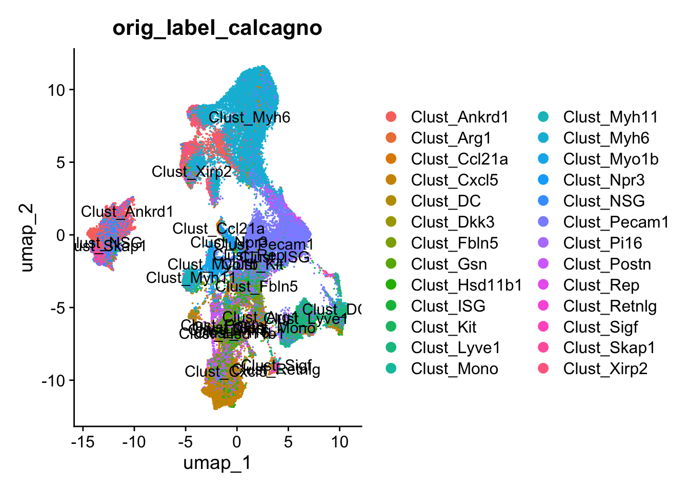

calcagno_lvl1 | calcagno_lvl2 | calcagno_lvl3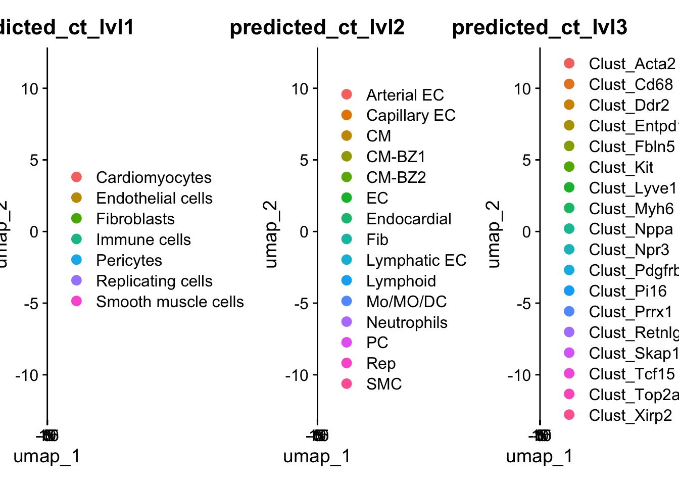

Use manual tissue annotation to improve endocardial cell labeling

Endocardial cells are very small and thin and form a monolayer at the inner lining of the heart. We noticed that our RNA marker Npr3 does not always reliably label endocardial cells and therefore will use manual annotation of the endocardial tissue regions to improve annotation of endocardial cells.

## Function to use GeoJson mask from QuPath with Seurat metadata to check cell overlap to manual annotation region
check_mask_overlap <- function(polygon_sf,metadata,img_height,anno_name){
  points_sf <- st_as_sf(metadata, coords = c("X_centroid", "Y_centroid"), crs = NA)
  polygon_sf <- st_set_crs(polygon_sf, NA)
  
  mirrored_geometries <- st_geometry(polygon_sf) %>% 
    st_coordinates() %>%
    as.data.frame() %>%
    mutate("Y" = img_height - Y) %>%
    select(X,Y,L2)
  mirrored_geometries <- as.data.frame(mirrored_geometries)
  
  polygon_list <- split(mirrored_geometries[,c("X", "Y")], mirrored_geometries$L2)
  closed_polys <- list()
  # Iterate over polygons in polygon_list and add the first row to the end of each polygon
  for (i in 1:length(polygon_list)) {
    closed_polys[[i]] <- as.matrix(rbind(polygon_list[[i]], polygon_list[[i]][1,]))
  }
  
  # Convert the list of polygons to sf objects
  sf_objects <- lapply(closed_polys, function(polygon) {
    st_polygon(list(polygon))
  })
  
  # Create a MULTIPOLYGON object
  multipolygon <- st_multipolygon(sf_objects)
  
  ## Check which points fall withing the annotation
  points_within_polygons <- st_within(points_sf, multipolygon, sparse = FALSE)
  metadata[anno_name] <- points_within_polygons
  return(metadata)
}

## Check which cells fall in the spatial endocardial region for each sample
all_vals <- list()
for(sample_id in unique(harmony_object@meta.data$sample_ID)){
  print(sample_id)
  image_sizes <- fread("./references/molkart.image_dimensions.csv")
  img_height <- subset(image_sizes,sample_ID == sample_id)$height
  
  polygon_sf <- st_read(paste("./annotations/molkart/heart_regions_r/",sample_id,".stack.geojson",sep=""))
  sample_meta <- subset(harmony_object@meta.data,sample_ID == sample_id)
  sample_vals <- list(polygon_sf,sample_meta,img_height)
  all_vals <- append(all_vals,list(sample_vals))
  #
}

[1] "sample_2d_r1_s1"
Reading layer `sample_2d_r1_s1.stack' from data source 
  `/Users/florian_wuennemann/1_Projects/MI_project/mi_spatialomics/annotations/molkart/heart_regions_r/sample_2d_r1_s1.stack.geojson' 
  using driver `GeoJSON'
Simple feature collection with 1 feature and 3 fields
Geometry type: POLYGON
Dimension:     XY
Bounding box:  xmin: 8566 ymin: 690 xmax: 13860 ymax: 9747
Geodetic CRS:  WGS 84
[1] "sample_2d_r2_s1"
Reading layer `sample_2d_r2_s1.stack' from data source 
  `/Users/florian_wuennemann/1_Projects/MI_project/mi_spatialomics/annotations/molkart/heart_regions_r/sample_2d_r2_s1.stack.geojson' 
  using driver `GeoJSON'
Simple feature collection with 3 features and 4 fields
Geometry type: POLYGON
Dimension:     XY
Bounding box:  xmin: 3793 ymin: 8044 xmax: 10720 ymax: 20387
Geodetic CRS:  WGS 84
[1] "sample_4d_r1_s1"
Reading layer `sample_4d_r1_s1.stack' from data source 
  `/Users/florian_wuennemann/1_Projects/MI_project/mi_spatialomics/annotations/molkart/heart_regions_r/sample_4d_r1_s1.stack.geojson' 
  using driver `GeoJSON'
Simple feature collection with 2 features and 4 fields
Geometry type: POLYGON
Dimension:     XY
Bounding box:  xmin: 5539 ymin: 1844 xmax: 10738 ymax: 12420
Geodetic CRS:  WGS 84
[1] "sample_4d_r2_s1"
Reading layer `sample_4d_r2_s1.stack' from data source 
  `/Users/florian_wuennemann/1_Projects/MI_project/mi_spatialomics/annotations/molkart/heart_regions_r/sample_4d_r2_s1.stack.geojson' 
  using driver `GeoJSON'
Simple feature collection with 3 features and 3 fields
Geometry type: POLYGON
Dimension:     XY
Bounding box:  xmin: 0 ymin: 236 xmax: 17963 ymax: 6159
Geodetic CRS:  WGS 84
[1] "sample_4h_r1_s1"
Reading layer `sample_4h_r1_s1.stack' from data source 
  `/Users/florian_wuennemann/1_Projects/MI_project/mi_spatialomics/annotations/molkart/heart_regions_r/sample_4h_r1_s1.stack.geojson' 
  using driver `GeoJSON'
Simple feature collection with 3 features and 3 fields
Geometry type: POLYGON
Dimension:     XY
Bounding box:  xmin: 2237 ymin: 5280 xmax: 15604 ymax: 17152
Geodetic CRS:  WGS 84
[1] "sample_4h_r2_s2"
Reading layer `sample_4h_r2_s2.stack' from data source 
  `/Users/florian_wuennemann/1_Projects/MI_project/mi_spatialomics/annotations/molkart/heart_regions_r/sample_4h_r2_s2.stack.geojson' 
  using driver `GeoJSON'
Simple feature collection with 1 feature and 2 fields
Geometry type: POLYGON
Dimension:     XY
Bounding box:  xmin: 6475 ymin: 3304 xmax: 18740 ymax: 15008
Geodetic CRS:  WGS 84
[1] "sample_control_r1_s1"
Reading layer `sample_control_r1_s1.stack' from data source 
  `/Users/florian_wuennemann/1_Projects/MI_project/mi_spatialomics/annotations/molkart/heart_regions_r/sample_control_r1_s1.stack.geojson' 
  using driver `GeoJSON'
Simple feature collection with 1 feature and 3 fields
Geometry type: POLYGON
Dimension:     XY
Bounding box:  xmin: 3748 ymin: 12539 xmax: 10117 ymax: 14892
Geodetic CRS:  WGS 84
[1] "sample_control_r2_s1"
Reading layer `sample_control_r2_s1.stack' from data source 
  `/Users/florian_wuennemann/1_Projects/MI_project/mi_spatialomics/annotations/molkart/heart_regions_r/sample_control_r2_s1.stack.geojson' 
  using driver `GeoJSON'
Simple feature collection with 3 features and 3 fields
Geometry type: POLYGON
Dimension:     XY
Bounding box:  xmin: 0 ymin: 2591 xmax: 6300 ymax: 7736
Geodetic CRS:  WGS 84

#test <- check_mask_overlap(polygon_sf,sample_meta,img_height)
meta_list <- Map(function(x) check_mask_overlap(x[[1]], x[[2]], x[[3]],"in_endo"), all_vals)

# Combine all data frames into one
new_full_meta <- do.call(rbind, meta_list)

## Which seurat cluster corresponds to endocardial cells (Npr3 positive)?
endocardial_cluster <- 15

## How many cells are in the endocardial cluster?
n_endo <- nrow(subset(new_full_meta,seurat_clusters == endocardial_cluster))

## How many of the transcriptionally defined endocardial cell cluster are spatially within the endocardium?
n_endo_spatial <- nrow(subset(new_full_meta,seurat_clusters == endocardial_cluster & in_endo == TRUE))

## How many segmented cells are total in the annotated regions?
anno_region_cells <- nrow(subset(new_full_meta, in_endo == TRUE))

## Let's classify cells that are Pecam1 positive within the endocardial region as endocardial (even if they are not Npr3 positive)
## add Pecam1 expression 
pecam1_exp <- harmony_object@assays$SCT@data["Pecam1",]
new_full_meta$Pecam1 <- pecam1_exp
npr3_exp <- harmony_object@assays$SCT@data["Npr3",]
new_full_meta$Npr3 <- npr3_exp

## How many cells are Pecam1 positive within the endocardial region?
pecam1_pos <- subset(new_full_meta,Pecam1 > 0 & in_endo == TRUE)

## Add another annotation column to metadata to classify all cells with Pecam1 > 0 within the endocardial region as endocardial cells
new_full_meta <- new_full_meta %>%
  mutate("spatial_endoc" = if_else((in_endo == TRUE & Pecam1 > 2) | (in_endo == TRUE & seurat_clusters == endocardial_cluster), TRUE,FALSE))

harmony_object@meta.data <- new_full_meta

Plot results of spatial annotation for endocardial cells

## Plot cells that are transcriptionally labeled as endocardial cells
ggplot(new_full_meta,aes(X_centroid,Y_centroid)) +
  geom_point(color = "darkgrey") +
  geom_point(data = subset(new_full_meta,seurat_clusters == endocardial_cluster),color = "red") +
  facet_wrap(~ sample_ID)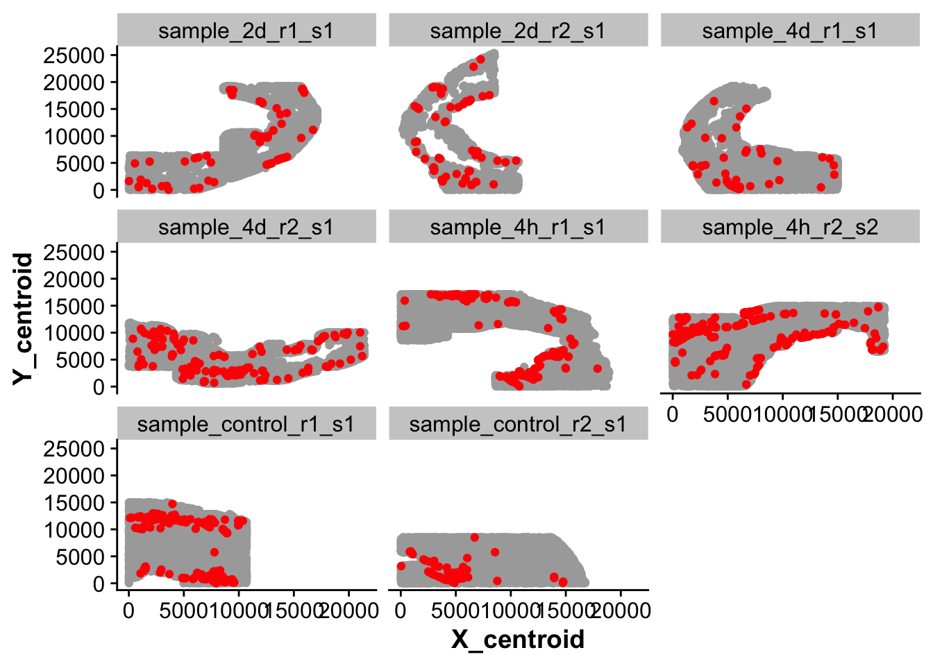

## Plot 
## 1: blue - originally transcriptionally labeled endocardial cells but not in endocardial region. 
## 2: red - transcriptionally labeled endocardial cells that were in endocardial region
## 3: purple - Cells that were not clustered with Npr3 positive cells but spatially fall within endocardium and are Pecam1 or Npr3 positive.
ggplot(new_full_meta,aes(X_centroid,Y_centroid)) +
  geom_point(color = "darkgrey", size = 0.5) +
  geom_point(data = subset(new_full_meta,spatial_endoc == TRUE & seurat_clusters == endocardial_cluster),color = "red", size = 0.75) +
  geom_point(data = subset(new_full_meta,spatial_endoc == TRUE & seurat_clusters != endocardial_cluster),color = "purple", size = 0.75) +
    geom_point(data = subset(new_full_meta,spatial_endoc == FALSE & seurat_clusters == endocardial_cluster),color = "blue", size = 0.75) +
  facet_wrap(~ sample_ID)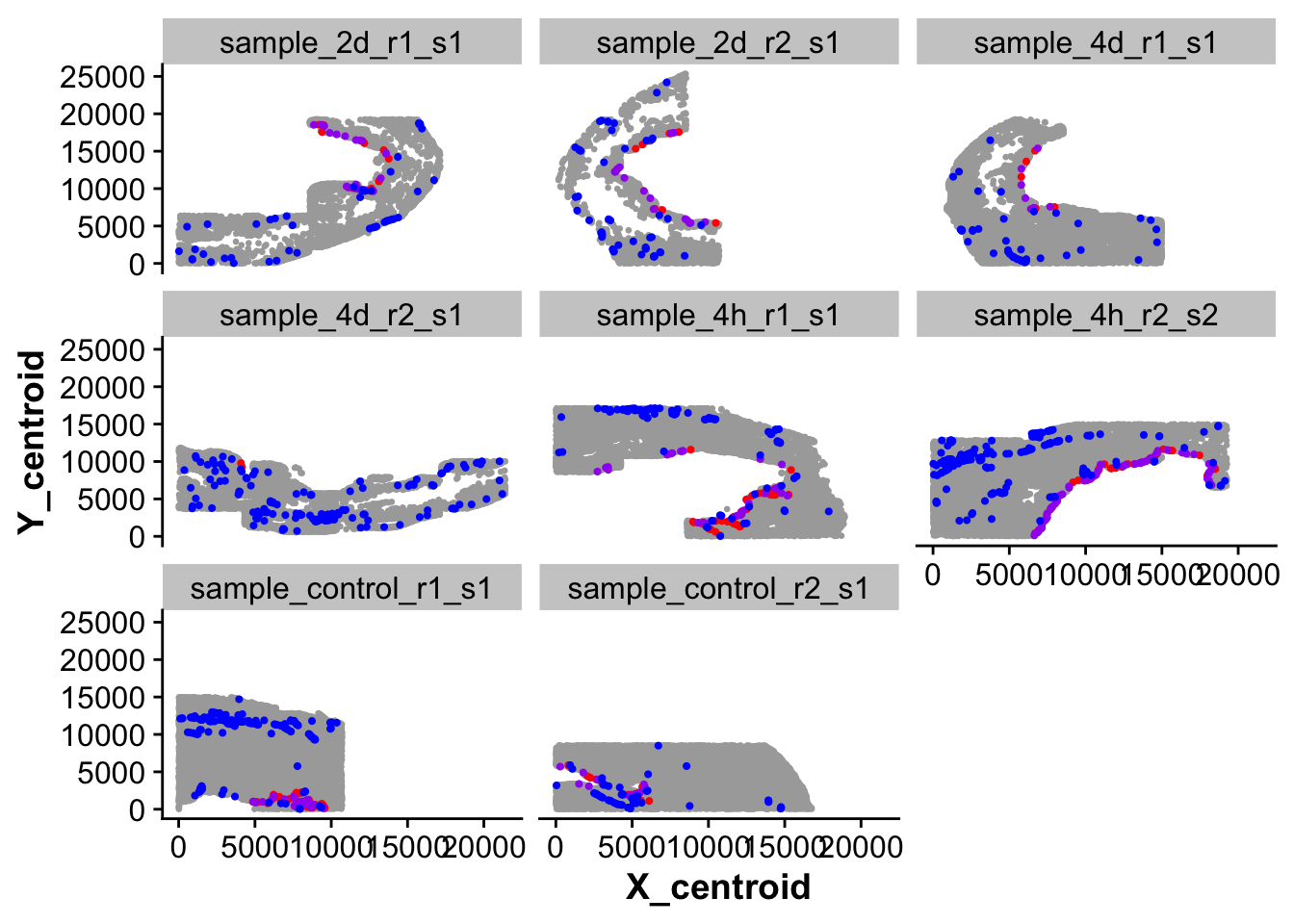

## Plot all cells that were considered "in endocardial region"
ggplot(new_full_meta,aes(X_centroid,Y_centroid)) +
  geom_point(color = "darkgrey") +
  geom_point(data = subset(new_full_meta,spatial_endoc == TRUE )) +
  facet_wrap(~ sample_ID)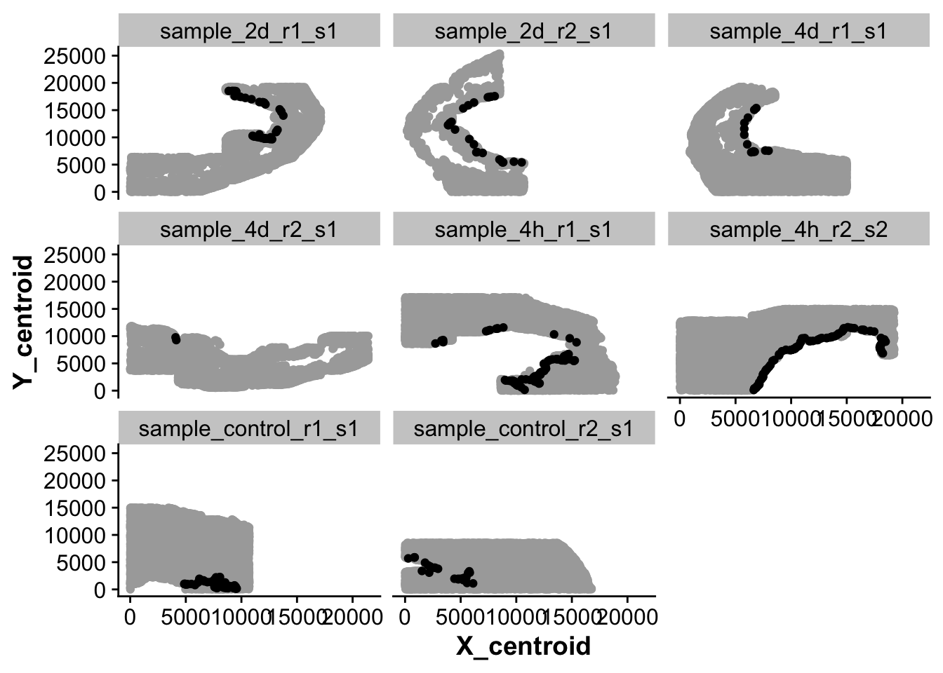

Assign cell-type names to clusters

Level 1 annotation - Higher cell types

## Annotate main cell-types and states
## LVL1
seurat_clusters <- harmony_object@active.ident

## Cluster level 1

new.cluster.ids <- c("Cardiomyocytes",  #0
                     "Endothelial_cells",  #1
                     "Cardiac_fibroblasts", #2
                     "Endothelial_cells", #3
                     "Cardiomyocytes", #4
                     "Cardiomyocytes", #5
                     "Cardiomyocytes", #6
                     "Cardiac_fibroblasts", #7
                     "Immune_cells", #8
                     "Immune_cells", #9 
                     "Immune_cells", #10
                     "Pericytes" , #11
                     "Cardiomyocytes", #12
                     "Smooth_muscle_cells", #13
                     "Cardiomyocytes", #14
                     "Endothelial_cells", #15 
                     "Immune_cells", #16
                     "Cardiomyocytes",#17
                     "Cardiomyocytes", #18 Glia_cells
                     "Immune_cells", #19
                     "Cardiomyocytes", #20
                     "Cardiac_fibroblasts", #21
                     "Immune_cells", #22
                     "Cardiac_fibroblasts" #23
                     )

names(new.cluster.ids) <- levels(harmony_object)
harmony_object <- RenameIdents(harmony_object, new.cluster.ids)
harmony_object@meta.data$anno_cell_type_lvl1 <- harmony_object@active.ident

## Reset cluster to seurat ID
Idents(object = harmony_object) <- "seurat_clusters"

DimPlot(harmony_object, reduction = "umap", label = TRUE, repel = TRUE,raster=FALSE, group.by = "anno_cell_type_lvl1")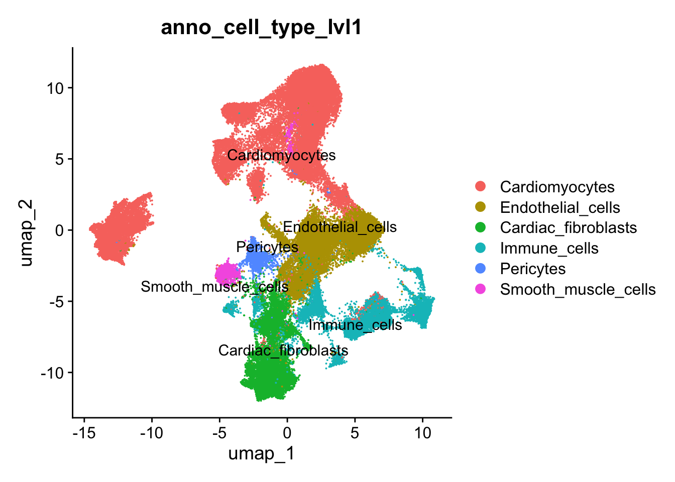

Level 2 annotation - Sub-Cell & cell states

## Annotate cell clusters with more detaile
## Lvl2

seurat_clusters <- harmony_object@active.ident

## Cluster level 2
new.cluster.ids <- c("Cardiomyocytes",  #0
                     "Endothelial_cells",  #1
                     "Cardiac_fibroblasts", #2
                     "Endothelial_cells", #3
                     "Cardiomyocytes", #4
                     "Cardiomyocytes_Nppa+", #5 Macrophages
                     "Cardiomyocytes", #6
                     "Cardiac_fibroblasts", #7
                     "Myeloid_cells", #8
                     "Myeloid_cells", #9
                     "Myeloid_cells", #10 Dendritic cells
                     "Pericytes" , #11
                     "Cardiomyocytes", #12
                     "Smooth_muscle_cells", #13
                     "Cardiomyocytes", #14
                     "Endocardial_cells", #15
                     "Myeloid_cells", #16
                     "Cardiomyocytes_Nppa+",#17
                     "Cardiomyocytes", #18
                     "Myeloid_cells", #19
                     "Cardiomyocytes_Nppa+", #20
                     "Cardiac_fibroblasts", #21
                     "Myeloid_cells", #22
                     "Cardiac_fibroblasts" #23
                     )

names(new.cluster.ids) <- levels(harmony_object)
harmony_object <- RenameIdents(harmony_object, new.cluster.ids)
harmony_object@meta.data$anno_cell_type_lvl2 <- harmony_object@active.ident

## Reset cluster to seurat ID
Idents(object = harmony_object) <- "seurat_clusters"

DimPlot(harmony_object, reduction = "umap", label = TRUE, repel = TRUE,raster=FALSE, group.by = "anno_cell_type_lvl2")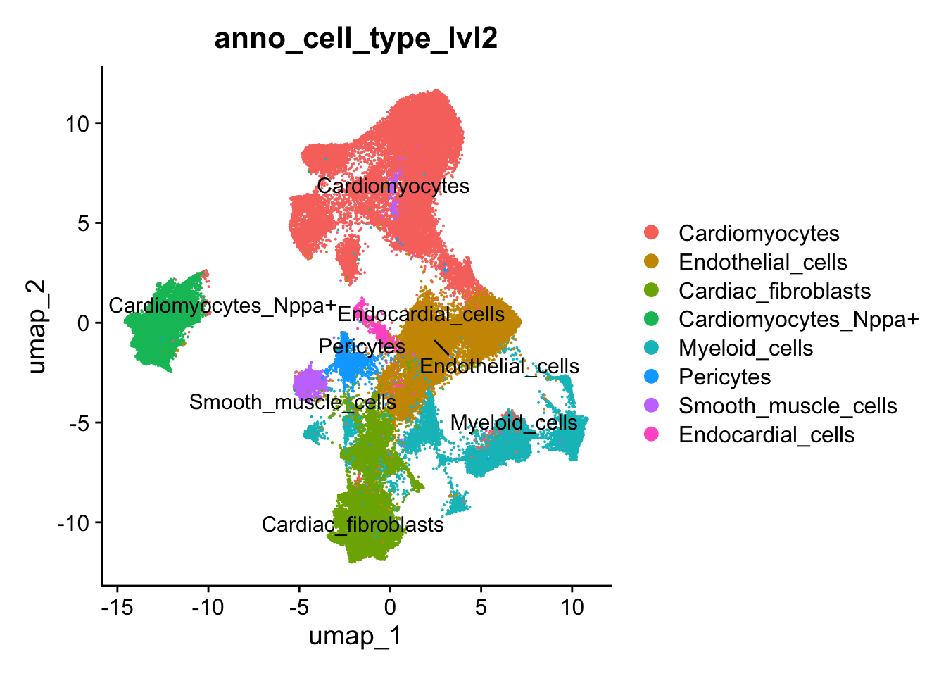

Level 3 annotation - Cell states with marker names

## Annotate cell clusters with more detailed cell states
## Lvl3
seurat_clusters <- harmony_object@active.ident

## Cluster level 3
new.cluster.ids <-  c("Cardiomyocytes_Pln",  #0
                     "Endothelial_cells_Kdr",  #1
                     "Cardiac_fibroblasts_Col1a1", #2
                     "Endothelial_cells_Aqp1", #3
                     "Cardiomyocytes_Pln", #4
                     "Cardiomyocytes_Nppa+", #5 Macrophages
                     "Cardiomyocytes_Cxcr6", #6
                     "Cardiac_fibroblasts_Dcn", #7
                     "Mono/Macros_C1qa", #8
                     "Mono/Macros_Arg1+", #9
                     "DC_Cd74", #10 Dendritic cells
                     "Pericytes_Colec11" , #11
                     "Cardiomyocytes_Nppb+", #12
                     "Smooth_muscle_cells_Myh11", #13
                     "Cardiomyocytes_Vegfa", #14
                     "Endocardial_cells_Npr3", #15
                     "Neutrophils_Csf3r", #16
                     "Cardiomyocytes_Nppa+",#17
                     "Cardiomyocytes_Pln", #18
                     "Mono/Macros_Ccl2", #19
                     "Cardiomyocytes_Nppa+", #20
                     "Cardiac_fibroblasts_Col1a1", #21
                     "Mono/Macros_C1qa", #22
                     "Cardiac_fibroblasts_Msln" #23
                     )


names(new.cluster.ids) <- levels(harmony_object)
harmony_object <- RenameIdents(harmony_object, new.cluster.ids)
harmony_object@meta.data$anno_cell_type_lvl3 <- harmony_object@active.ident

## Reset cluster to seurat ID
Idents(object = harmony_object) <- "seurat_clusters"

DimPlot(harmony_object, reduction = "umap", label = TRUE, repel = TRUE,raster=FALSE, group.by = "anno_cell_type_lvl3")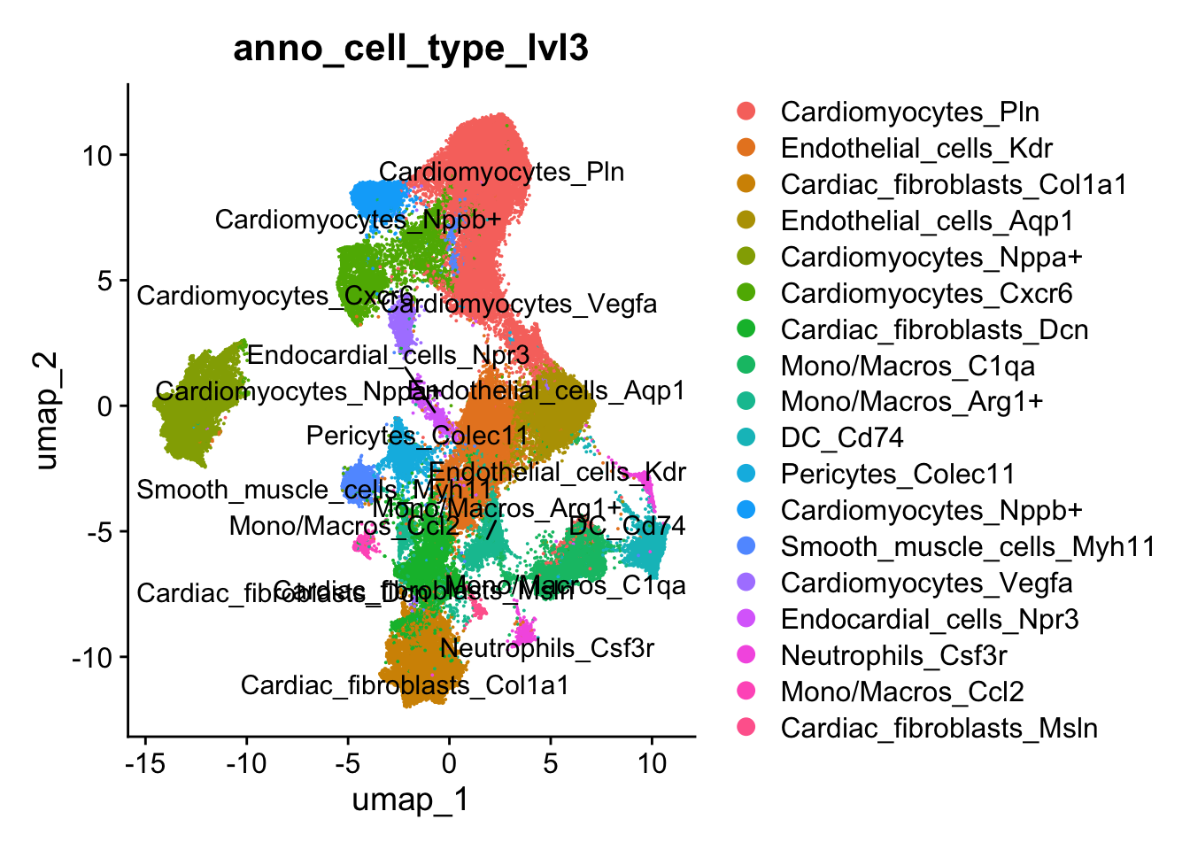

Refine cell type cluster based on spatial annotation and marker expression

## Using the clustering settings we did, there is a subgroup of cells that are lymphoid but clustered with cells in cluster 16. We will put these cells in a separate cluster based on their marker expression
new_full_meta <- harmony_object@meta.data
emb <- harmony_object@reductions$umap@cell.embeddings
lymph_emb <- subset(as.data.frame(emb),umap_1 > 8.5 & umap_2 > -5)

new_full_meta <- new_full_meta %>%
  mutate("lymphoid" = if_else(rownames(new_full_meta) %in% rownames(lymph_emb) & seurat_clusters == 16, TRUE,FALSE))

harmony_object@meta.data <- new_full_meta

harmony_object@meta.data <- harmony_object@meta.data %>%
  mutate("anno_cell_type_lvl2" = if_else(lymphoid == TRUE, "Lymphoid_cells",anno_cell_type_lvl2),
         "anno_cell_type_lvl3" = if_else(lymphoid == TRUE, "Lymphoid_cells_Cd3e",anno_cell_type_lvl3)
         )

## Endocardial cells
## First, let's reclassify endocardial cells based on the Qupath annotation we did above
harmony_object@meta.data <- harmony_object@meta.data %>%
  mutate("anno_cell_type_lvl2" = if_else(spatial_endoc == TRUE & anno_cell_type_lvl2 == "Endocardial_cells","Endocardial_cells",
                                         if_else(spatial_endoc == TRUE & anno_cell_type_lvl2 != "Endocardial_cells","Endocardial_cells",
                                          if_else(spatial_endoc == FALSE & anno_cell_type_lvl2 == "Endocardial_cells","Endothelial_cells",anno_cell_type_lvl2))),
         "anno_cell_type_lvl3" = if_else(spatial_endoc == TRUE & anno_cell_type_lvl3 == "Endocardial_cells_Npr3","Endocardial_cells_Npr3",
                                         if_else(spatial_endoc == TRUE & anno_cell_type_lvl3 != "Endocardial_cells_Npr3","Endocardial_cells_Npr3",
                                         if_else(spatial_endoc == FALSE & anno_cell_type_lvl3 == "Endocardial_cells_Npr3","Lymphatic_endothelial_cells_Lyve1",anno_cell_type_lvl3))))


# ## Add cells located within endocardium to annotations
# harmony_object@meta.data <- harmony_object@meta.data %>%
#   mutate("anno_cell_type_lvl2" = if_else(spatial_endoc == TRUE | anno_cell_type_lvl2 == "Endocardial_cells","Endocardial_cells",anno_cell_type_lvl2),
#          "anno_cell_type_lvl3" = if_else(spatial_endoc == TRUE | anno_cell_type_lvl3 == "Endocardial_cells_Npr3","Endocardial_cells_Npr3",anno_cell_type_lvl3))

new_full_meta <- harmony_object@meta.data
## Plot cells that are 
ggplot(new_full_meta,aes(X_centroid,Y_centroid)) +
  geom_point(color = "darkgrey") +
  geom_point(data = subset(new_full_meta,anno_cell_type_lvl2 == "Endocardial_cells"),color = "red") +
  geom_point(data = subset(new_full_meta,grepl("Myeloid_cells",anno_cell_type_lvl2)),color = "blue") +
  facet_wrap(~ sample_ID)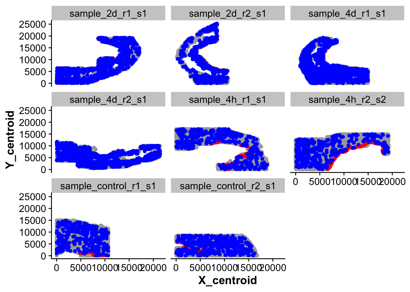

p1 <- DimPlot(harmony_object, reduction = "umap", group.by = "anno_cell_type_lvl1",raster=FALSE, 
              alpha = 0.5, label = TRUE, repel = TRUE) + NoLegend()
p2 <- DimPlot(harmony_object, reduction = "umap", group.by = "anno_cell_type_lvl2",raster=FALSE, 
              alpha = 0.5, label = TRUE, repel = TRUE) + NoLegend() 
p3 <- DimPlot(harmony_object, reduction = "umap", group.by = "anno_cell_type_lvl3",raster=FALSE, 
              alpha = 0.5, label = TRUE, repel = TRUE) + NoLegend()

p1 + p2 + p3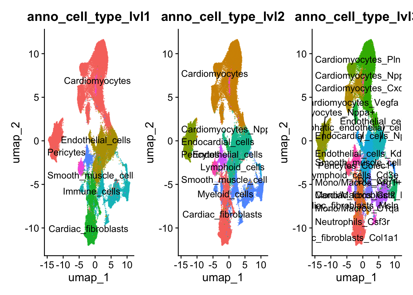

Identify and plot best “marker” genes

Idents(object = harmony_object) <- "anno_cell_type_lvl2"
harmony_object <- PrepSCTFindMarkers(harmony_object, assay = "SCT", verbose = TRUE)

Found 4 SCT models. Recorrecting SCT counts using minimum median counts: 78

harmony_markers <- FindAllMarkers(harmony_object, logfc.threshold = 0.5, only.pos = TRUE)

Calculating cluster Myeloid_cells

Calculating cluster Cardiac_fibroblasts

Calculating cluster Pericytes

Calculating cluster Endothelial_cells

Calculating cluster Cardiomyocytes

Calculating cluster Smooth_muscle_cells

Calculating cluster Cardiomyocytes_Nppa+

Calculating cluster Endocardial_cells

Calculating cluster Lymphoid_cells

## Set order of cell types
levels(harmony_object) <- rev(sort(levels(harmony_object)))

library(viridis)
genes <- c("Csf3r","Npr3","Ccl2","Lyz2","H2-Eb1",
           "Pdgfrb","Nppa","Nppb","C1qa","Postn","Aqp1","Mybpc3")
DotPlot(harmony_object, group.by = "anno_cell_type_lvl2",
        features = genes) +
  geom_point(aes(size=pct.exp), shape = 21, colour="black", stroke=0.75) +
  scale_colour_viridis(option="magma", direction = 1)

Warning: The following variables were found in both object meta data and the default assay: Npr3
Returning meta data; if you want the feature, please use the assay's key (eg. sct_Npr3)

Scale for colour is already present.
Adding another scale for colour, which will replace the existing scale.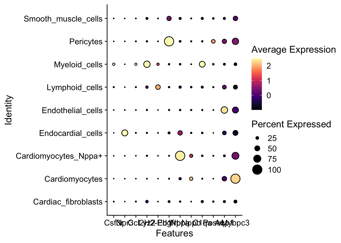

Save object as seurat RDS

saveRDS(harmony_object,
        file = "./output/molkart/molkart.seurat_object.rds")

# ## If the object has already been computed we can load it
# harmony_object <- readRDS(file
#                           = "./output/molkart/molkart.seurat_object.rds")

Save data formatted for input to spatial anndata object

metadata <- harmony_object@meta.data %>%
  mutate("liana_cts" = if_else(grepl("Myeloid_cells",anno_cell_type_lvl2),"Myeloid_cells",anno_cell_type_lvl2))

coordinates <- metadata %>% select(X_centroid,Y_centroid)
counts <- t(as.matrix(harmony_object@assays$SCT@counts))

## Save coordinates
write.table(coordinates,
            "./output/molkart/harmony_object.coordinates_anndata.tsv",
            sep="\t",
            col.names = FALSE,
            row.names = FALSE,
            quote = FALSE)

## Save counts
write.table(counts,
            "./output/molkart/harmony_object.counts_anndata.tsv",
            sep="\t",
            col.names = TRUE,
            row.names = FALSE,
            quote = FALSE)

## Annotation
write.table(metadata,
            "./output/molkart/harmony_object.metadata_anndata.tsv",
            sep="\t",
            col.names = TRUE,
            row.names = FALSE,
            quote = FALSE)

Generate Misty input

misty_in <- harmony_object@meta.data %>%
  dplyr::select(sample_ID,timepoint,replicate,X_centroid,Y_centroid,Area,anno_cell_type_lvl1,anno_cell_type_lvl2,anno_cell_type_lvl3,nCount_RNA) 
misty_in$cell_ID <- rownames(misty_in)

expression_plot_list <- list()

# final_samples <- c("sample_control_r1_s1","sample_control_r2_s1",
#                    "sample_4h_r1_s1","sample_4h_r2_s2",
#                    "sample_2d_r1_s1","sample_2d_r2_s1",
#                    "sample_4d_r1_s1","sample_4d_r2_s1")

samples <- c("sample_control_r1_s1","sample_4h_r1_s1",
             "sample_2d_r1_s1","sample_4d_r1_s1",
             "sample_control_r2_s1","sample_4h_r2_s2",
             "sample_2d_r2_s1","sample_4d_r2_s1")

for(this_sample in samples){
  pt_size <- 0.2
  cluster_of_int <- c(16,19)
  sample_object <- subset(misty_in,sample_ID == this_sample)
  
  highlight_plot <- ggplot(sample_object,aes(X_centroid,Y_centroid)) +
    geom_point(aes(color = anno_cell_type_lvl2),size = pt_size) +
    theme_classic() +
    labs(x = "Spatial 1",
         y = "Spatial 2",
         title = this_sample) +
    theme(axis.ticks = element_blank(),
            axis.text = element_blank(),
            legend.position = "right") +
    scale_color_brewer(palette = "Set3")
  
      expression_plot_list[[this_sample]] <- highlight_plot
  
}

wrap_plots(expression_plot_list, nrow = 2, ncol = 4)  + plot_layout(guides = 'collect')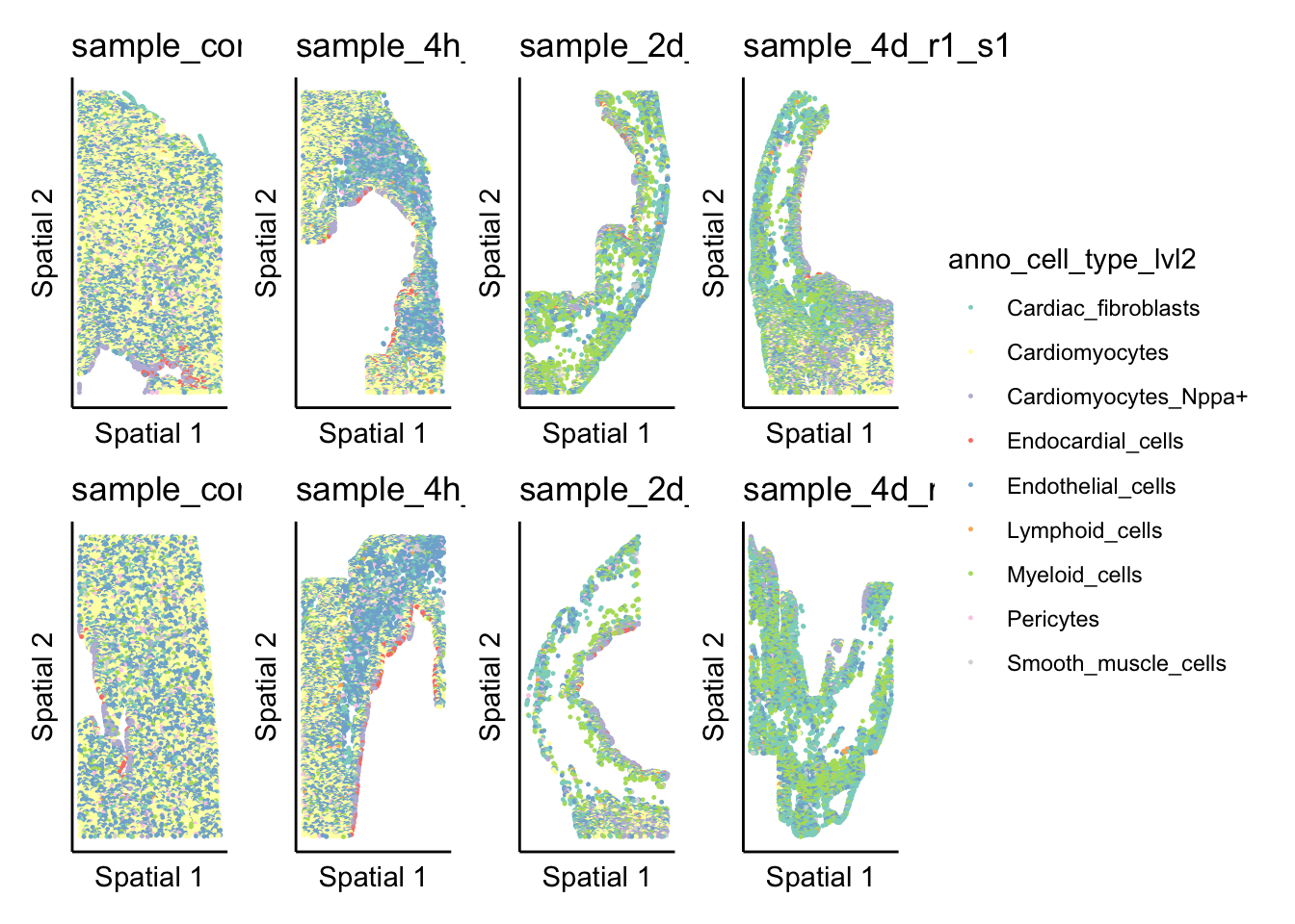

misty_in_lowres <- misty_in %>%
  mutate("misty_cts" = anno_cell_type_lvl2)

write.table(misty_in_lowres,
            file = "./output/molkart/molkart.misty_celltype_table.lowres.tsv",
            sep="\t",
            col.names = TRUE,
            row.names = FALSE,
            quote = FALSE)

misty_in_highres <- misty_in %>%
  mutate("misty_cts" = anno_cell_type_lvl3)

write.table(misty_in_highres,
            file = "./output/molkart/molkart.misty_celltype_table.highres.tsv",
            sep="\t",
            col.names = TRUE,
            row.names = FALSE,
            quote = FALSE)

Session information

sessionInfo()

R version 4.3.1 (2023-06-16)
Platform: aarch64-apple-darwin20 (64-bit)
Running under: macOS Sonoma 14.1.2

Matrix products: default
BLAS:   /Library/Frameworks/R.framework/Versions/4.3-arm64/Resources/lib/libRblas.0.dylib 
LAPACK: /Library/Frameworks/R.framework/Versions/4.3-arm64/Resources/lib/libRlapack.dylib;  LAPACK version 3.11.0

locale:
[1] en_US.UTF-8/en_US.UTF-8/en_US.UTF-8/C/en_US.UTF-8/en_US.UTF-8

time zone: Europe/Berlin
tzcode source: internal

attached base packages:
[1] stats     graphics  grDevices datasets  utils     methods   base     

other attached packages:
 [1] RColorBrewer_1.1-3    ggsci_3.0.0           cowplot_1.1.2        
 [4] viridis_0.6.4         viridisLite_0.4.2     sfheaders_0.4.4      
 [7] sf_1.0-15             Matrix_1.6-5          GGally_2.2.0         
[10] lubridate_1.9.3       forcats_1.0.0         stringr_1.5.1        
[13] dplyr_1.1.4           purrr_1.0.2           readr_2.1.5          
[16] tidyr_1.3.0           tibble_3.2.1          tidyverse_2.0.0      
[19] Nebulosa_1.12.0       patchwork_1.2.0       ggplot2_3.4.4        
[22] here_1.0.1            harmony_1.2.0         Rcpp_1.0.12          
[25] data.table_1.14.10    SeuratDisk_0.0.0.9021 SeuratData_0.2.2.9001
[28] Seurat_5.0.1          SeuratObject_5.0.1    sp_2.1-2             
[31] workflowr_1.7.1      

loaded via a namespace (and not attached):
  [1] fs_1.6.3                    matrixStats_1.2.0          
  [3] spatstat.sparse_3.0-3       bitops_1.0-7               
  [5] httr_1.4.7                  tools_4.3.1                
  [7] sctransform_0.4.1           utf8_1.2.4                 
  [9] R6_2.5.1                    lazyeval_0.2.2             
 [11] uwot_0.1.16                 withr_2.5.2                
 [13] gridExtra_2.3               progressr_0.14.0           
 [15] textshaping_0.3.7           cli_3.6.2                  
 [17] Biobase_2.62.0              spatstat.explore_3.2-5     
 [19] fastDummies_1.7.3           labeling_0.4.3             
 [21] sass_0.4.8                  mvtnorm_1.2-4              
 [23] spatstat.data_3.0-3         proxy_0.4-27               
 [25] ggridges_0.5.5              pbapply_1.7-2              
 [27] systemfonts_1.0.5           parallelly_1.36.0          
 [29] limma_3.58.1                rstudioapi_0.15.0          
 [31] generics_0.1.3              ica_1.0-3                  
 [33] spatstat.random_3.2-2       ggbeeswarm_0.7.2           
 [35] fansi_1.0.6                 S4Vectors_0.40.2           
 [37] abind_1.4-5                 lifecycle_1.0.4            
 [39] whisker_0.4.1               yaml_2.3.8                 
 [41] SummarizedExperiment_1.32.0 SparseArray_1.2.3          
 [43] Rtsne_0.17                  glmGamPoi_1.14.0           
 [45] grid_4.3.1                  promises_1.2.1             
 [47] crayon_1.5.2                miniUI_0.1.1.1             
 [49] lattice_0.22-5              pillar_1.9.0               
 [51] knitr_1.45                  GenomicRanges_1.54.1       
 [53] future.apply_1.11.1         codetools_0.2-19           
 [55] leiden_0.4.3.1              glue_1.7.0                 
 [57] getPass_0.2-4               vctrs_0.6.5                
 [59] png_0.1-8                   spam_2.10-0                
 [61] gtable_0.3.4                cachem_1.0.8               
 [63] ks_1.14.2                   xfun_0.41                  
 [65] S4Arrays_1.2.0              mime_0.12                  
 [67] pracma_2.4.4                survival_3.5-7             
 [69] SingleCellExperiment_1.24.0 units_0.8-5                
 [71] statmod_1.5.0               ellipsis_0.3.2             
 [73] fitdistrplus_1.1-11         ROCR_1.0-11                
 [75] nlme_3.1-164                bit64_4.0.5                
 [77] RcppAnnoy_0.0.21            GenomeInfoDb_1.38.5        
 [79] rprojroot_2.0.4             bslib_0.6.1                
 [81] irlba_2.3.5.1               vipor_0.4.7                
 [83] KernSmooth_2.23-22          colorspace_2.1-0           
 [85] BiocGenerics_0.48.1         DBI_1.2.0                  
 [87] ggrastr_1.0.2               tidyselect_1.2.0           
 [89] processx_3.8.3              bit_4.0.5                  
 [91] compiler_4.3.1              git2r_0.33.0               
 [93] hdf5r_1.3.8                 DelayedArray_0.28.0        
 [95] plotly_4.10.4               scales_1.3.0               
 [97] classInt_0.4-10             lmtest_0.9-40              
 [99] callr_3.7.3                 rappdirs_0.3.3             
[101] digest_0.6.34               goftest_1.2-3              
[103] presto_1.0.0                spatstat.utils_3.0-4       
[105] rmarkdown_2.25              XVector_0.42.0             
[107] RhpcBLASctl_0.23-42         htmltools_0.5.7            
[109] pkgconfig_2.0.3             sparseMatrixStats_1.14.0   
[111] MatrixGenerics_1.14.0       highr_0.10                 
[113] fastmap_1.1.1               rlang_1.1.3                
[115] htmlwidgets_1.6.4           shiny_1.8.0                
[117] DelayedMatrixStats_1.24.0   farver_2.1.1               
[119] jquerylib_0.1.4             zoo_1.8-12                 
[121] jsonlite_1.8.8              mclust_6.0.1               
[123] RCurl_1.98-1.14             magrittr_2.0.3             
[125] GenomeInfoDbData_1.2.11     dotCall64_1.1-1            
[127] munsell_0.5.0               reticulate_1.34.0          
[129] stringi_1.8.3               zlibbioc_1.48.0            
[131] MASS_7.3-60.0.1             plyr_1.8.9                 
[133] ggstats_0.5.1               parallel_4.3.1             
[135] listenv_0.9.0               ggrepel_0.9.5              
[137] deldir_2.0-2                splines_4.3.1              
[139] tensor_1.5                  hms_1.1.3                  
[141] ps_1.7.6                    igraph_1.6.0               
[143] spatstat.geom_3.2-7         RcppHNSW_0.5.0             
[145] reshape2_1.4.4              stats4_4.3.1               
[147] evaluate_0.23               renv_1.0.3                 
[149] BiocManager_1.30.22         tzdb_0.4.0                 
[151] httpuv_1.6.14               RANN_2.6.1                 
[153] polyclip_1.10-6             future_1.33.1              
[155] scattermore_1.2             xtable_1.8-4               
[157] e1071_1.7-14                RSpectra_0.16-1            
[159] later_1.3.2                 class_7.3-22               
[161] ragg_1.2.7                  beeswarm_0.4.0             
[163] IRanges_2.36.0              cluster_2.1.6              
[165] timechange_0.2.0            globals_0.16.2