Visium Plot Overlay Toy Example

import squidpy as sq
import matplotlib.pyplot as plt

# 1. Load a public Visium dataset
adata = sq.datasets.visium_fluo_adata()
print(adata)  # Basic info

# Inspect available images and scalefactors
library_id = list(adata.uns['spatial'].keys())[0]
adata.uns['spatial'][library_id]['scalefactors']

AnnData object with n_obs × n_vars = 2800 × 16562
    obs: 'in_tissue', 'array_row', 'array_col', 'n_genes_by_counts', 'log1p_n_genes_by_counts', 'total_counts', 'log1p_total_counts', 'pct_counts_in_top_50_genes', 'pct_counts_in_top_100_genes', 'pct_counts_in_top_200_genes', 'pct_counts_in_top_500_genes', 'total_counts_MT', 'log1p_total_counts_MT', 'pct_counts_MT', 'n_counts', 'leiden', 'cluster'
    var: 'gene_ids', 'feature_types', 'genome', 'MT', 'n_cells_by_counts', 'mean_counts', 'log1p_mean_counts', 'pct_dropout_by_counts', 'total_counts', 'log1p_total_counts', 'n_cells', 'highly_variable', 'highly_variable_rank', 'means', 'variances', 'variances_norm'
    uns: 'cluster_colors', 'hvg', 'leiden', 'leiden_colors', 'neighbors', 'pca', 'spatial', 'umap'
    obsm: 'X_pca', 'X_umap', 'spatial'
    varm: 'PCs'
    obsp: 'connectivities', 'distances'

{'fiducial_diameter_fullres': np.float64(288.25050000000005),
 'spot_diameter_fullres': np.float64(178.44077999999996),
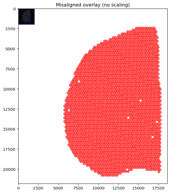
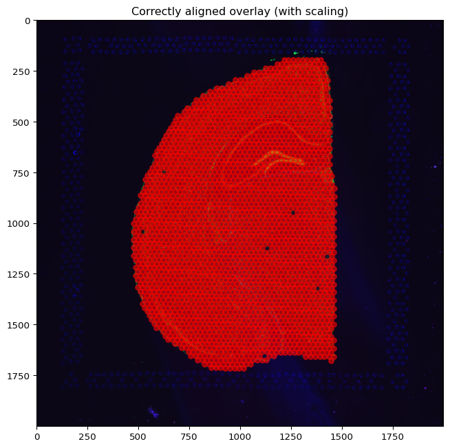
 'tissue_hires_scalef': np.float64(0.08250825),
 'tissue_lowres_scalef': np.float64(0.024752475)}

# Extract image (hires)
img = adata.uns['spatial'][library_id]['images']['hires']

# Unscaled coordinates
coords_unscaled = adata.obsm['spatial']

# Display the histology image
fig, ax = plt.subplots(figsize=(8, 8))
ax.imshow(img)

# Try plotting directly (we do not want this graph)
fig, ax = plt.subplots(figsize=(8, 8))
ax.imshow(img)
ax.scatter(coords_unscaled[:, 0], coords_unscaled[:, 1],
           s=30, c='red', alpha=0.6)
ax.set_title("Misaligned overlay (no scaling)")
plt.show()

# Get scale factor for hires image
scale = adata.uns['spatial'][library_id]['scalefactors']['tissue_hires_scalef']

# Apply scaling
coords_scaled = adata.obsm['spatial'] * scale

# Correct overlay
fig, ax = plt.subplots(figsize=(8, 8))
ax.imshow(img)
ax.scatter(coords_scaled[:, 0], coords_scaled[:, 1],
           s=30, c='red', alpha=0.6)
ax.set_title("Correctly aligned overlay (with scaling)")
# ax.invert_yaxis()  # sometimes needed
plt.show()

# Overlay gene expression data
gene = "Gad1"
fig, ax = plt.subplots(figsize=(8, 8))
ax.imshow(img)
sc = ax.scatter(coords_scaled[:, 0], coords_scaled[:, 1],
                c=adata[:, gene].X.toarray().flatten(),
                cmap='magma', s=30)
ax.set_title(f"{gene} expression aligned to tissue")
# ax.invert_yaxis() 
plt.colorbar(sc, ax=ax)
plt.show()