Species Barretts Relationships
Last updated: 2021-04-15
Checks: 7 0
Knit directory: esoph-micro-cancer-workflow/
This reproducible R Markdown analysis was created with workflowr (version 1.6.2). The Checks tab describes the reproducibility checks that were applied when the results were created. The Past versions tab lists the development history.
Great! Since the R Markdown file has been committed to the Git repository, you know the exact version of the code that produced these results.
Great job! The global environment was empty. Objects defined in the global environment can affect the analysis in your R Markdown file in unknown ways. For reproduciblity it’s best to always run the code in an empty environment.
The command set.seed(20200916) was run prior to running the code in the R Markdown file. Setting a seed ensures that any results that rely on randomness, e.g. subsampling or permutations, are reproducible.
Great job! Recording the operating system, R version, and package versions is critical for reproducibility.
Nice! There were no cached chunks for this analysis, so you can be confident that you successfully produced the results during this run.
Great job! Using relative paths to the files within your workflowr project makes it easier to run your code on other machines.
Great! You are using Git for version control. Tracking code development and connecting the code version to the results is critical for reproducibility.
The results in this page were generated with repository version b11a4b5. See the Past versions tab to see a history of the changes made to the R Markdown and HTML files.
Note that you need to be careful to ensure that all relevant files for the analysis have been committed to Git prior to generating the results (you can use wflow_publish or wflow_git_commit). workflowr only checks the R Markdown file, but you know if there are other scripts or data files that it depends on. Below is the status of the Git repository when the results were generated:
Ignored files:
    Ignored:    .Rhistory
    Ignored:    .Rproj.user/
    Ignored:    data/

Untracked files:
    Untracked:  analysis/picrust-campy.Rmd
    Untracked:  analysis/picrust-fuso.Rmd
    Untracked:  analysis/picrust-prevo.Rmd
    Untracked:  analysis/picrust-strepto.Rmd
    Untracked:  code/results-question-1.Rmd
    Untracked:  code/results-question-2.Rmd
    Untracked:  code/results-question-3.Rmd
    Untracked:  output/picrust_ec_stratefied_campy_data_results.csv
    Untracked:  output/picrust_ec_stratefied_fuso_data_results.csv
    Untracked:  output/picrust_ec_stratefied_prevo_data_results.csv
    Untracked:  output/picrust_ec_stratefied_strepto_data_results.csv
    Untracked:  output/picrust_ko_stratefied_campy_data_results.csv
    Untracked:  output/picrust_ko_stratefied_fuso_data_results.csv
    Untracked:  output/picrust_ko_stratefied_prevo_data_results.csv
    Untracked:  output/picrust_ko_stratefied_strepto_data_results.csv

Unstaged changes:
    Modified:   analysis/index.Rmd
    Modified:   analysis/picrust-analyses.Rmd
    Deleted:    analysis/results-question-1.Rmd
    Deleted:    analysis/results-question-2.Rmd
    Deleted:    analysis/results-question-3.Rmd
Note that any generated files, e.g. HTML, png, CSS, etc., are not included in this status report because it is ok for generated content to have uncommitted changes.
These are the previous versions of the repository in which changes were made to the R Markdown (analysis/species-sample-type-combined.Rmd) and HTML (docs/species-sample-type-combined.html) files. If you’ve configured a remote Git repository (see ?wflow_git_remote), click on the hyperlinks in the table below to view the files as they were in that past version.
| File | Version | Author | Date | Message |
|---|---|---|---|---|
| Rmd | b11a4b5 | noah-padgett | 2021-03-25 | updated picrust analyses and results figures |
| Rmd | 56180cd | noah-padgett | 2021-03-14 | updated analyses and violin plots |
| html | 56180cd | noah-padgett | 2021-03-14 | updated analyses and violin plots |
| Rmd | 092bf33 | noah-padgett | 2021-02-25 | fixed group error in violin plots |
| html | 092bf33 | noah-padgett | 2021-02-25 | fixed group error in violin plots |
| Rmd | f91e666 | noah-padgett | 2021-02-25 | violin updates |
| html | f91e666 | noah-padgett | 2021-02-25 | violin updates |
| Rmd | 13f1528 | alisonjung | 2021-02-18 | Barretts violin plot updates |
| Rmd | fe971b9 | noah-padgett | 2021-02-13 | violin plot scale fixed |
| Rmd | 285a2fb | noah-padgett | 2021-02-10 | updated violion plots |
| html | 285a2fb | noah-padgett | 2021-02-10 | updated violion plots |
Violin Plot Fuso
# merge datasets by subsetting to specific variables then merging
analysis.dat <- dat.16s.s %>%
  dplyr::mutate(ID = as.factor(accession.number)) %>%
  dplyr::select(OTU, sample_type, Abundance, ID, source)

dat <- dat.rna.s %>%
  dplyr::select(OTU, sample_type, Abundance, ID, source)
analysis.dat <- full_join(analysis.dat, dat)

dat <- dat.wgs.s %>%
  dplyr::select(OTU, sample_type, Abundance, ID, source)

analysis.dat <- full_join(analysis.dat, dat) %>%
  mutate(pres = ifelse(Abundance > 0, 1, 0)) %>%
  filter(OTU=="Fusobacterium nucleatum")# create a presence/absences variable


tb <- analysis.dat %>%
  filter(is.na(sample_type)==F)%>%
  group_by(sample_type, OTU) %>%
  summarise(
    N=n(),
    p = sum(pres, na.rm=T),
    percent = p/N*100
  )

kable(tb, format="html")%>%
kable_styling(full_width = T)| sample_type | OTU | N | p | percent |
|---|---|---|---|---|
| 16SrRNA Barrett’s (BO) | Fusobacterium nucleatum | 5 | 3 | 60.00000 |
| 16SrRNA Non-tumor (w/ Barrett’s history) | Fusobacterium nucleatum | 43 | 19 | 44.18605 |
| 16SrRNA Tumor (w/ Barrett’s history) | Fusobacterium nucleatum | 35 | 16 | 45.71429 |
| RNA-seq Non-tumor (w/ Barrett’s history) | Fusobacterium nucleatum | 3 | 2 | 66.66667 |
| RNA-seq Tumor (w/ Barrett’s history) | Fusobacterium nucleatum | 26 | 5 | 19.23077 |
| WGS Non-tumor (w/ Barrett’s history) | Fusobacterium nucleatum | 6 | 2 | 33.33333 |
| WGS Tumor (w/ Barrett’s history) | Fusobacterium nucleatum | 4 | 2 | 50.00000 |
analysis.dat <- analysis.dat %>%
  filter(is.na(sample_type)==F)%>%
  mutate(
    Abund = Abundance*100
  )

#root function
root<-function(x){
  x <- ifelse(x < 0, 0, x)
  x**(0.2)
}
#inverse root function
invroot<-function(x){
  x**(5)
}

# colors
cols <- c("16SrRNA Tumor (w/ Barrett's history)" = "#C0392B",
          "16SrRNA Non-tumor (w/ Barrett's history)"= "#336699",
          "16SrRNA Barrett's (BO)"= "#229667",
          "RNA-seq Tumor (w/ Barrett's history)"= "#C0392B",
          "RNA-seq Non-tumor (w/ Barrett's history)"= "#336699",
          "WGS Non-tumor (w/ Barrett's history)"= "#336699",
          "WGS Tumor (w/ Barrett's history) " = "#C0392B")
# "#2C3E50", "#2980B9", "#8E44AD", "#C0392B", "#D35400", "#F39C12", "#F1C40F", "#27AE60", "#196f3e"
#   mycolors = c()
#   mycolors$Tissue["T"]   = "#C0392B"
#   mycolors$Tissue["N"]   = "#336699"
#   mycolors$Tissue["BO"]  = "#229667"


p <- ggplot(analysis.dat, aes(sample_type, Abund, color=sample_type)) +
  geom_violin(scale="width", adjust=0.5)+
  geom_point(alpha=0.75)+
  scale_y_continuous(
    trans=scales::trans_new("root", root, invroot),
    breaks=c(0, 0.001,0.01, 0.1, 1,10,50, 100),
    labels = c(0, 0.001,0.01, 0.1, 1,10,50, 100),
    limits = c(0, 110)
  )+
  scale_color_manual(values=cols)+
  annotate(
    "text", x=c(1:7), y=c(rep(110, 7)),
    label=c(paste0(round(tb[1,5], 0),"% (",tb[1,4],"/",tb[1,3],")"),
            paste0(round(tb[2,5], 0),"% (",tb[2,4],"/",tb[2,3],")"),
            paste0(round(tb[3,5], 0),"% (",tb[3,4],"/",tb[3,3],")"),
            paste0(round(tb[4,5], 0),"% (",tb[4,4],"/",tb[4,3],")"),
            paste0(round(tb[5,5], 0),"% (",tb[5,4],"/",tb[5,3],")"),
            paste0(round(tb[6,5], 0),"% (",tb[6,4],"/",tb[6,3],")"),
            paste0(round(tb[7,5], 0),"% (",tb[7,4],"/",tb[7,3],")"))
  )+
  labs(x=NULL, y="% Abundance")+
  theme(
    axis.text.x = element_text(angle=30, hjust=0.95, vjust=0.95),
    legend.position = "none"
  )
p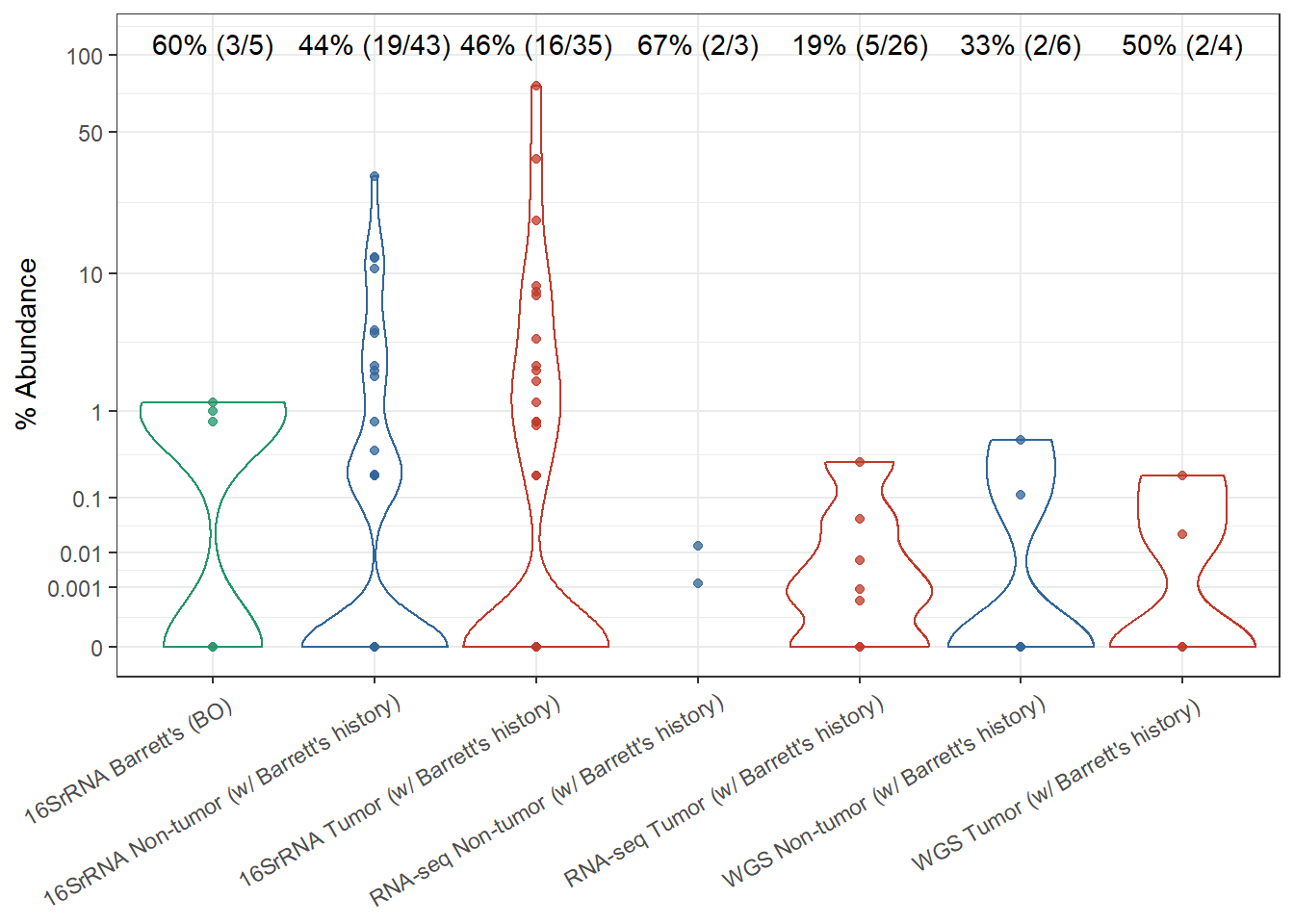
ggsave("output/Barretts_violin-fuso.pdf", p, units = "in", width = 10, height = 6)Violin Plot Strepto
# merge datasets by subsetting to specific variables then merging
analysis.dat <- dat.16s.s %>%
  dplyr::mutate(ID = as.factor(accession.number)) %>%
  dplyr::select(OTU, sample_type, Abundance, ID, source)

dat <- dat.rna.s %>%
  dplyr::select(OTU, sample_type, Abundance, ID, source)
analysis.dat <- full_join(analysis.dat, dat)

dat <- dat.wgs.s %>%
  dplyr::select(OTU, sample_type, Abundance, ID, source)

analysis.dat <- full_join(analysis.dat, dat) %>%
  mutate(pres = ifelse(Abundance > 0, 1, 0)) %>%
  filter(OTU%like%"Streptococcus")# create a presence/absences variable


tb <- analysis.dat %>%
  filter(is.na(sample_type)==F)%>%
  group_by(sample_type, OTU) %>%
  summarise(
    N=n(),
    p = sum(pres, na.rm=T),
    percent = p/N*100
  )

kable(tb, format="html")%>%
kable_styling(full_width = T)| sample_type | OTU | N | p | percent |
|---|---|---|---|---|
| 16SrRNA Barrett’s (BO) | Streptococcus spp. (not uniquely identified) | 5 | 5 | 100.00000 |
| 16SrRNA Non-tumor (w/ Barrett’s history) | Streptococcus spp. (not uniquely identified) | 43 | 41 | 95.34884 |
| 16SrRNA Tumor (w/ Barrett’s history) | Streptococcus spp. (not uniquely identified) | 35 | 33 | 94.28571 |
| RNA-seq Non-tumor (w/ Barrett’s history) | Streptococcus sanguinis | 3 | 2 | 66.66667 |
| RNA-seq Tumor (w/ Barrett’s history) | Streptococcus sanguinis | 26 | 6 | 23.07692 |
| WGS Non-tumor (w/ Barrett’s history) | Streptococcus sanguinis | 6 | 2 | 33.33333 |
| WGS Tumor (w/ Barrett’s history) | Streptococcus sanguinis | 4 | 2 | 50.00000 |
analysis.dat <- analysis.dat %>%
  filter(is.na(sample_type)==F)%>%
  mutate(
    Abund = Abundance*100
  )

#root function
root<-function(x){
  x <- ifelse(x < 0, 0, x)
  x**(0.2)
}
#inverse root function
invroot<-function(x){
  x**(5)
}

p <- ggplot(analysis.dat, aes(sample_type, Abund)) +
  geom_violin(scale="width", adjust=2)+
  geom_point(alpha=0.75)+
  scale_y_continuous(
    trans=scales::trans_new("root", root, invroot),
    breaks=c(0, 0.001,0.01, 0.1, 1,10,50, 100),
    labels = c(0, 0.001,0.01, 0.1, 1,10,50, 100),
    limits = c(0, 110)
  )+
  annotate(
    "text", x=c(1:7), y=c(rep(110, 7)),
    label=c(paste0(round(tb[1,5], 0),"% (",tb[1,4],"/",tb[1,3],")"),
            paste0(round(tb[2,5], 0),"% (",tb[2,4],"/",tb[2,3],")"),
            paste0(round(tb[3,5], 0),"% (",tb[3,4],"/",tb[3,3],")"),
            paste0(round(tb[4,5], 0),"% (",tb[4,4],"/",tb[4,3],")"),
            paste0(round(tb[5,5], 0),"% (",tb[5,4],"/",tb[5,3],")"),
            paste0(round(tb[6,5], 0),"% (",tb[6,4],"/",tb[6,3],")"),
            paste0(round(tb[7,5], 0),"% (",tb[7,4],"/",tb[7,3],")"))
  )+
  labs(x=NULL, y="% Abundance")+
  theme(
    axis.text.x = element_text(angle=30, hjust=0.95, vjust=0.95)
  )
p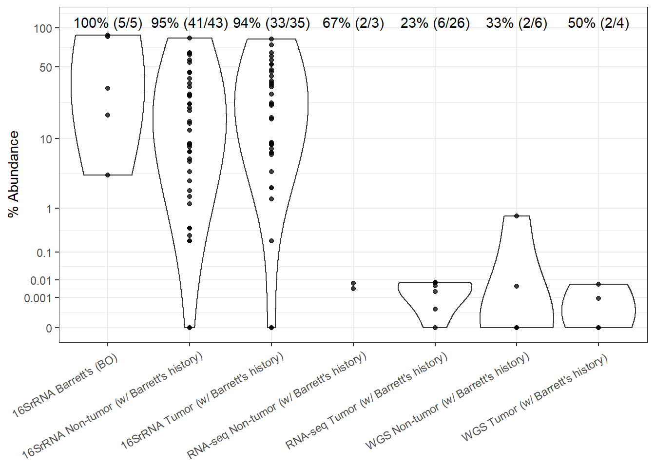
ggsave("output/Barretts_violin-strepto.pdf", p, units = "in", width = 10, height = 6)Violin Plot Campy
# merge datasets by subsetting to specific variables then merging
analysis.dat <- dat.16s.s %>%
  dplyr::mutate(ID = as.factor(accession.number)) %>%
  dplyr::select(OTU, sample_type, Abundance, ID, source)

dat <- dat.rna.s %>%
  dplyr::select(OTU, sample_type, Abundance, ID, source)
analysis.dat <- full_join(analysis.dat, dat)

dat <- dat.wgs.s %>%
  dplyr::select(OTU, sample_type, Abundance, ID, source)

analysis.dat <- full_join(analysis.dat, dat) %>%
  mutate(pres = ifelse(Abundance > 0, 1, 0)) %>%
  filter(OTU %like% "Campylobacter")# create a presence/absences variable


tb <- analysis.dat %>%
  filter(is.na(sample_type)==F)%>%
  group_by(sample_type, OTU) %>%
  summarise(
    N=n(),
    p = sum(pres, na.rm=T),
    percent = p/N*100
  )

kable(tb, format="html")%>%
kable_styling(full_width = T)| sample_type | OTU | N | p | percent |
|---|---|---|---|---|
| 16SrRNA Barrett’s (BO) | Campylobacter spp. (not uniquely identified) | 5 | 2 | 40.000000 |
| 16SrRNA Non-tumor (w/ Barrett’s history) | Campylobacter spp. (not uniquely identified) | 43 | 6 | 13.953488 |
| 16SrRNA Tumor (w/ Barrett’s history) | Campylobacter spp. (not uniquely identified) | 35 | 9 | 25.714286 |
| RNA-seq Non-tumor (w/ Barrett’s history) | Campylobacter concisus | 3 | 0 | 0.000000 |
| RNA-seq Tumor (w/ Barrett’s history) | Campylobacter concisus | 26 | 1 | 3.846154 |
| WGS Non-tumor (w/ Barrett’s history) | Campylobacter concisus | 6 | 1 | 16.666667 |
| WGS Tumor (w/ Barrett’s history) | Campylobacter concisus | 4 | 2 | 50.000000 |
analysis.dat <- analysis.dat %>%
  filter(is.na(sample_type)==F)%>%
  mutate(
    Abund = Abundance*100
  )

#root function
root<-function(x){
  x <- ifelse(x < 0, 0, x)
  x**(0.2)
}
#inverse root function
invroot<-function(x){
  x**(5)
}

p <- ggplot(analysis.dat, aes(sample_type, Abund)) +
  geom_violin(scale="width", adjust=2)+
  geom_point(alpha=0.75)+
  scale_y_continuous(
    trans=scales::trans_new("root", root, invroot),
    breaks=c(0, 0.001,0.01, 0.1, 1,10,50, 100),
    labels = c(0, 0.001,0.01, 0.1, 1,10,50, 100),
    limits = c(0, 110)
  )+
  annotate(
    "text", x=c(1:7), y=c(rep(110, 7)),
    label=c(paste0(round(tb[1,5], 0),"% (",tb[1,4],"/",tb[1,3],")"),
            paste0(round(tb[2,5], 0),"% (",tb[2,4],"/",tb[2,3],")"),
            paste0(round(tb[3,5], 0),"% (",tb[3,4],"/",tb[3,3],")"),
            paste0(round(tb[4,5], 0),"% (",tb[4,4],"/",tb[4,3],")"),
            paste0(round(tb[5,5], 0),"% (",tb[5,4],"/",tb[5,3],")"),
            paste0(round(tb[6,5], 0),"% (",tb[6,4],"/",tb[6,3],")"),
            paste0(round(tb[7,5], 0),"% (",tb[7,4],"/",tb[7,3],")"))
  )+
  labs(x=NULL, y="% Abundance")+
  theme(
    axis.text.x = element_text(angle=30, hjust=0.95, vjust=0.95)
  )
p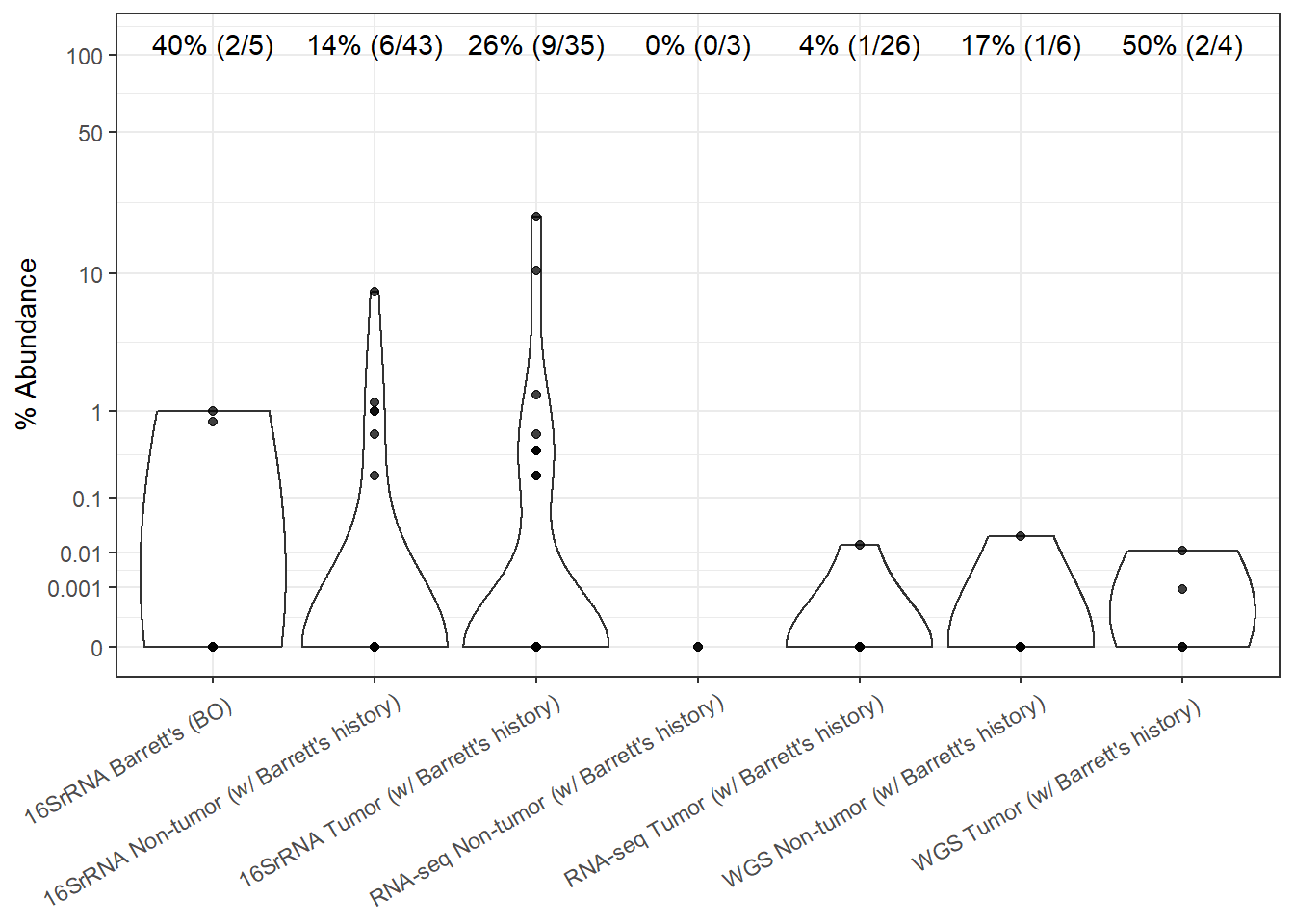
ggsave("output/Barretts_violin-campy.pdf", p, units = "in", width = 10, height = 6)Violin Plot Prevo
# merge datasets by subsetting to specific variables then merging
analysis.dat <- dat.16s.s %>%
  dplyr::mutate(ID = as.factor(accession.number)) %>%
  dplyr::select(OTU, sample_type, Abundance, ID, source)

dat <- dat.rna.s %>%
  dplyr::select(OTU, sample_type, Abundance, ID, source)
analysis.dat <- full_join(analysis.dat, dat)

dat <- dat.wgs.s %>%
  dplyr::select(OTU, sample_type, Abundance, ID, source)

analysis.dat <- full_join(analysis.dat, dat) %>%
  mutate(pres = ifelse(Abundance > 0, 1, 0)) %>%
  filter(OTU %like% "Prevotella")# create a presence/absences variable


tb <- analysis.dat %>%
  filter(is.na(sample_type)==F)%>%
  group_by(sample_type, OTU) %>%
  summarise(
    N=n(),
    p = sum(pres, na.rm=T),
    percent = p/N*100
  )

kable(tb, format="html")%>%
kable_styling(full_width = T)| sample_type | OTU | N | p | percent |
|---|---|---|---|---|
| 16SrRNA Barrett’s (BO) | Prevotella spp. | 5 | 4 | 80.00000 |
| 16SrRNA Non-tumor (w/ Barrett’s history) | Prevotella spp. | 43 | 28 | 65.11628 |
| 16SrRNA Tumor (w/ Barrett’s history) | Prevotella spp. | 35 | 27 | 77.14286 |
| RNA-seq Non-tumor (w/ Barrett’s history) | Prevotella denticola | 3 | 1 | 33.33333 |
| RNA-seq Non-tumor (w/ Barrett’s history) | Prevotella intermedia | 3 | 2 | 66.66667 |
| RNA-seq Non-tumor (w/ Barrett’s history) | Prevotella melaninogenica | 3 | 2 | 66.66667 |
| RNA-seq Non-tumor (w/ Barrett’s history) | Prevotella ruminicola | 3 | 1 | 33.33333 |
| RNA-seq Tumor (w/ Barrett’s history) | Prevotella denticola | 26 | 4 | 15.38462 |
| RNA-seq Tumor (w/ Barrett’s history) | Prevotella intermedia | 26 | 3 | 11.53846 |
| RNA-seq Tumor (w/ Barrett’s history) | Prevotella melaninogenica | 26 | 5 | 19.23077 |
| RNA-seq Tumor (w/ Barrett’s history) | Prevotella ruminicola | 26 | 0 | 0.00000 |
| WGS Non-tumor (w/ Barrett’s history) | Prevotella denticola | 6 | 1 | 16.66667 |
| WGS Non-tumor (w/ Barrett’s history) | Prevotella intermedia | 6 | 2 | 33.33333 |
| WGS Non-tumor (w/ Barrett’s history) | Prevotella melaninogenica | 6 | 1 | 16.66667 |
| WGS Non-tumor (w/ Barrett’s history) | Prevotella ruminicola | 6 | 0 | 0.00000 |
| WGS Tumor (w/ Barrett’s history) | Prevotella denticola | 4 | 1 | 25.00000 |
| WGS Tumor (w/ Barrett’s history) | Prevotella intermedia | 4 | 1 | 25.00000 |
| WGS Tumor (w/ Barrett’s history) | Prevotella melaninogenica | 4 | 3 | 75.00000 |
| WGS Tumor (w/ Barrett’s history) | Prevotella ruminicola | 4 | 0 | 0.00000 |
analysis.dat <- analysis.dat %>%
  filter(is.na(sample_type)==F)%>%
  mutate(
    Abund = Abundance*100
  )

#root function
root<-function(x){
  x <- ifelse(x < 0, 0, x)
  x**(0.2)
}
#inverse root function
invroot<-function(x){
  x**(5)
}

p <- ggplot(analysis.dat, aes(sample_type, Abund)) +
  geom_violin(scale="width", adjust=2)+
  geom_point(alpha=0.75)+
  scale_y_continuous(
    trans=scales::trans_new("root", root, invroot),
    breaks=c(0, 0.001,0.01, 0.1, 1,10,50, 100),
    labels = c(0, 0.001,0.01, 0.1, 1,10,50, 100),
    limits = c(0, 110)
  )+
  annotate(
    "text", x=c(1:7), y=c(rep(110, 7)),
    label=c(paste0(round(tb[1,5], 0),"% (",tb[1,4],"/",tb[1,3],")"),
            paste0(round(tb[2,5], 0),"% (",tb[2,4],"/",tb[2,3],")"),
            paste0(round(tb[3,5], 0),"% (",tb[3,4],"/",tb[3,3],")"),
            paste0(round(tb[4,5], 0),"% (",tb[4,4],"/",tb[4,3],")"),
            paste0(round(tb[5,5], 0),"% (",tb[5,4],"/",tb[5,3],")"),
            paste0(round(tb[6,5], 0),"% (",tb[6,4],"/",tb[6,3],")"),
            paste0(round(tb[7,5], 0),"% (",tb[7,4],"/",tb[7,3],")"))
  )+
  labs(x=NULL, y="% Abundance")+
  theme(
    axis.text.x = element_text(angle=30, hjust=0.95, vjust=0.95)
  )
p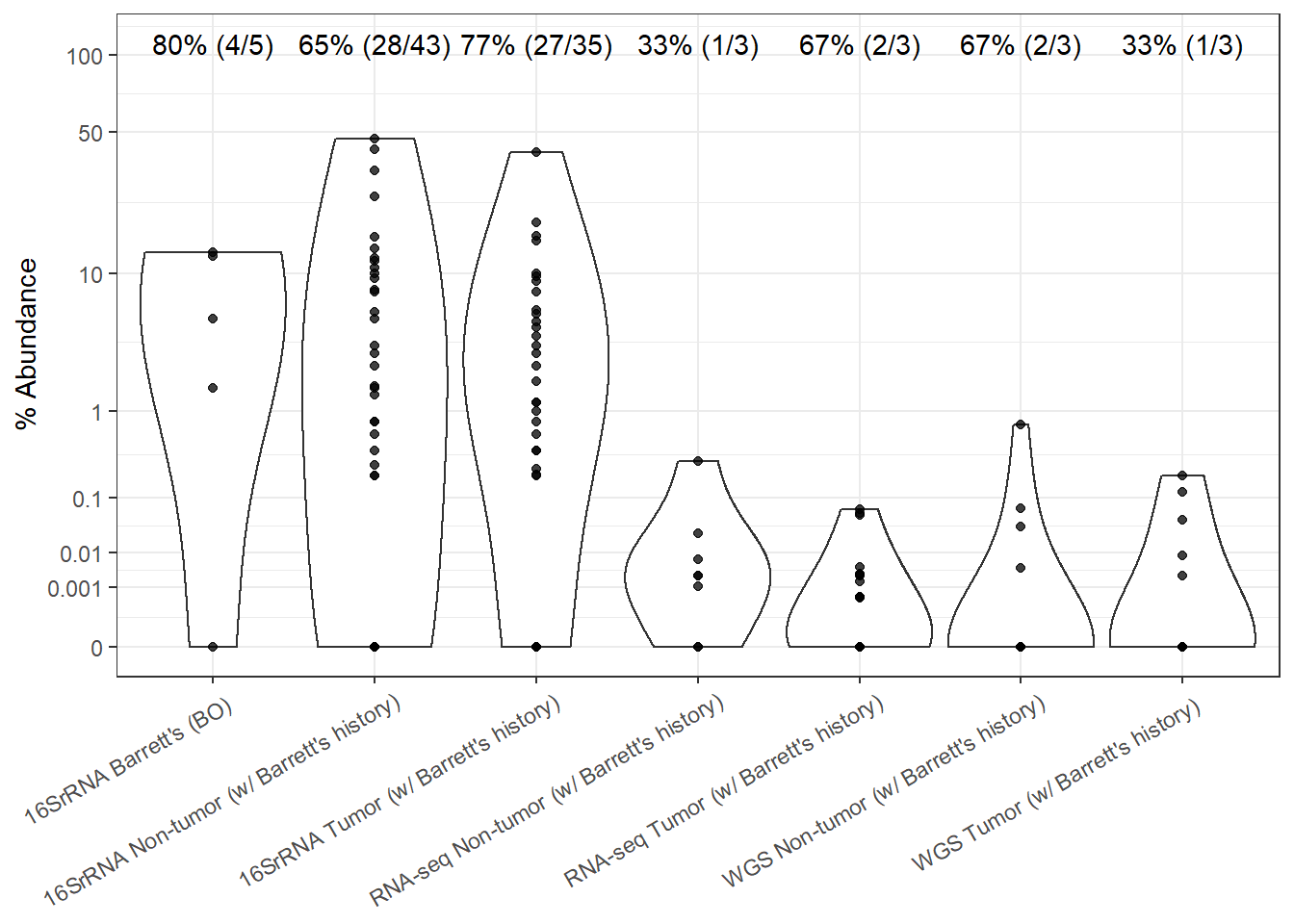
ggsave("output/Barretts_violin-prevo.pdf", p, units = "in", width = 10, height = 6)
sessionInfo()R version 4.0.5 (2021-03-31)
Platform: x86_64-w64-mingw32/x64 (64-bit)
Running under: Windows 10 x64 (build 19042)
Matrix products: default
locale:
[1] LC_COLLATE=English_United States.1252
[2] LC_CTYPE=English_United States.1252
[3] LC_MONETARY=English_United States.1252
[4] LC_NUMERIC=C
[5] LC_TIME=English_United States.1252
attached base packages:
[1] stats graphics grDevices utils datasets methods base
other attached packages:
[1] cowplot_1.1.1 dendextend_1.14.0 ggdendro_0.1.22 reshape2_1.4.4
[5] car_3.0-10 carData_3.0-4 gvlma_1.0.0.3 patchwork_1.1.1
[9] viridis_0.5.1 viridisLite_0.3.0 gridExtra_2.3 xtable_1.8-4
[13] kableExtra_1.3.4 MASS_7.3-53.1 data.table_1.14.0 readxl_1.3.1
[17] forcats_0.5.1 stringr_1.4.0 dplyr_1.0.5 purrr_0.3.4
[21] readr_1.4.0 tidyr_1.1.3 tibble_3.1.0 ggplot2_3.3.3
[25] tidyverse_1.3.0 lmerTest_3.1-3 lme4_1.1-26 Matrix_1.3-2
[29] vegan_2.5-7 lattice_0.20-41 permute_0.9-5 phyloseq_1.34.0
[33] workflowr_1.6.2
loaded via a namespace (and not attached):
[1] minqa_1.2.4 colorspace_2.0-0 rio_0.5.26
[4] ellipsis_0.3.1 rprojroot_2.0.2 XVector_0.30.0
[7] fs_1.5.0 rstudioapi_0.13 farver_2.1.0
[10] fansi_0.4.2 lubridate_1.7.10 xml2_1.3.2
[13] codetools_0.2-18 splines_4.0.5 knitr_1.31
[16] ade4_1.7-16 jsonlite_1.7.2 nloptr_1.2.2.2
[19] broom_0.7.5 cluster_2.1.1 dbplyr_2.1.0
[22] BiocManager_1.30.10 compiler_4.0.5 httr_1.4.2
[25] backports_1.2.1 assertthat_0.2.1 cli_2.3.1
[28] later_1.1.0.1 htmltools_0.5.1.1 prettyunits_1.1.1
[31] tools_4.0.5 igraph_1.2.6 gtable_0.3.0
[34] glue_1.4.2 Rcpp_1.0.6 Biobase_2.50.0
[37] cellranger_1.1.0 jquerylib_0.1.3 vctrs_0.3.6
[40] Biostrings_2.58.0 rhdf5filters_1.2.0 multtest_2.46.0
[43] svglite_2.0.0 ape_5.4-1 nlme_3.1-152
[46] iterators_1.0.13 xfun_0.21 ps_1.6.0
[49] openxlsx_4.2.3 rvest_1.0.0 lifecycle_1.0.0
[52] statmod_1.4.35 zlibbioc_1.36.0 scales_1.1.1
[55] hms_1.0.0 promises_1.2.0.1 parallel_4.0.5
[58] biomformat_1.18.0 rhdf5_2.34.0 curl_4.3
[61] yaml_2.2.1 sass_0.3.1 stringi_1.5.3
[64] highr_0.8 S4Vectors_0.28.1 foreach_1.5.1
[67] BiocGenerics_0.36.0 zip_2.1.1 boot_1.3-27
[70] systemfonts_1.0.1 rlang_0.4.10 pkgconfig_2.0.3
[73] evaluate_0.14 Rhdf5lib_1.12.1 tidyselect_1.1.0
[76] plyr_1.8.6 magrittr_2.0.1 R6_2.5.0
[79] IRanges_2.24.1 generics_0.1.0 DBI_1.1.1
[82] foreign_0.8-81 pillar_1.5.1 haven_2.3.1
[85] whisker_0.4 withr_2.4.1 mgcv_1.8-34
[88] abind_1.4-5 survival_3.2-10 modelr_0.1.8
[91] crayon_1.4.1 utf8_1.1.4 rmarkdown_2.7
[94] progress_1.2.2 grid_4.0.5 git2r_0.28.0
[97] webshot_0.5.2 reprex_1.0.0 digest_0.6.27
[100] httpuv_1.5.5 numDeriv_2016.8-1.1 stats4_4.0.5
[103] munsell_0.5.0 bslib_0.2.4