Results Output for Question 1
Last updated: 2021-01-14
Checks: 6 1
Knit directory: esoph-micro-cancer-workflow/
This reproducible R Markdown analysis was created with workflowr (version 1.6.2). The Checks tab describes the reproducibility checks that were applied when the results were created. The Past versions tab lists the development history.
The R Markdown is untracked by Git. To know which version of the R Markdown file created these results, you’ll want to first commit it to the Git repo. If you’re still working on the analysis, you can ignore this warning. When you’re finished, you can run wflow_publish to commit the R Markdown file and build the HTML.
Great job! The global environment was empty. Objects defined in the global environment can affect the analysis in your R Markdown file in unknown ways. For reproduciblity it’s best to always run the code in an empty environment.
The command set.seed(20200916) was run prior to running the code in the R Markdown file. Setting a seed ensures that any results that rely on randomness, e.g. subsampling or permutations, are reproducible.
Great job! Recording the operating system, R version, and package versions is critical for reproducibility.
Nice! There were no cached chunks for this analysis, so you can be confident that you successfully produced the results during this run.
Great job! Using relative paths to the files within your workflowr project makes it easier to run your code on other machines.
Great! You are using Git for version control. Tracking code development and connecting the code version to the results is critical for reproducibility.
The results in this page were generated with repository version 1d24c1f. See the Past versions tab to see a history of the changes made to the R Markdown and HTML files.
Note that you need to be careful to ensure that all relevant files for the analysis have been committed to Git prior to generating the results (you can use wflow_publish or wflow_git_commit). workflowr only checks the R Markdown file, but you know if there are other scripts or data files that it depends on. Below is the status of the Git repository when the results were generated:
Ignored files:
    Ignored:    .Rhistory
    Ignored:    .Rproj.user/
    Ignored:    analysis/figure/
    Ignored:    data/

Untracked files:
    Untracked:  analysis/data-check-for-RNAscope.Rmd
    Untracked:  analysis/results-question-1.Rmd
    Untracked:  analysis/results-question-2.Rmd
    Untracked:  code/barrets-stacked-plot.Rmd

Unstaged changes:
    Modified:   analysis/index.Rmd
    Modified:   analysis/test-of-replication.Rmd
Note that any generated files, e.g. HTML, png, CSS, etc., are not included in this status report because it is ok for generated content to have uncommitted changes.
There are no past versions. Publish this analysis with wflow_publish() to start tracking its development.
Question 1
Q1: is there a taxonomic signature shared between the barrett's samples?- Heatmap of relative abundance supervised by sample type: Barrett’s (BO), tumor-adjacent EAC-w/history of barrett’s, EAC-w/ history of barrett’s
- Stacked bar chart of phylum and genus abundance by sample type, same as above
- Additional comparison in TCGA; EAC w/history of Barrett’s vs EAC w/ no history of Barrett’s; same analyses as above
Summary of observations
NCI 16s data
# in long format
table(dat.16s$sample_type)
                                      0                           Barretts Only
                                  19800                                    1320
EAC-adjacent tissue w/ Barretts History         EAC tissues w/ Barretts History
                                  11352                                    9240
dat <- dat.16s %>% filter(OTU == "Fusobacterium_nucleatum")
table(dat$sample_type)
                                      0                           Barretts Only
                                     75                                       5
EAC-adjacent tissue w/ Barretts History         EAC tissues w/ Barretts History
                                     43                                      35
table(dat$Barretts.)
 N  Y
71 87
5 Barretts samples that were non-EAC tissue related.
TCGA RNAseq data
# in long format
table(dat.rna$sample_type)
                                      0 EAC-adjacent tissue w/ Barretts History
                                 112176                                    2337
        EAC tissues w/ Barretts History
                                  20254
dat <- dat.rna %>% filter(otu2 == "Fusobacterium nucleatum")
table(dat$sample_type)
                                      0 EAC-adjacent tissue w/ Barretts History
                                    144                                       3
        EAC tissues w/ Barretts History
                                     26
table(dat$Barrett.s.Esophagus.Reported)
           No Not Available           Yes
          113            31            29
TCGA WGS data
# in long format
table(dat.wgs$sample_type)
                                      0 EAC-adjacent tissue w/ Barretts History
                                 100491                                    4674
        EAC tissues w/ Barretts History
                                   3116
dat <- dat.wgs %>% filter(otu2 == "Fusobacterium nucleatum")
table(dat$sample_type)
                                      0 EAC-adjacent tissue w/ Barretts History
                                    129                                       6
        EAC tissues w/ Barretts History
                                      4
table(dat$Barrett.s.Esophagus.Reported)
           No Not Available           Yes
           54            47            10
Heatmaps
All OTUs (RA > 0.001)
plot.dat <- dat.16s %>% filter(sample_type != "0", Abundance > 0.001) %>%
  mutate(ID = as.factor(accession.number),
         Genus = substr(Genus, 4, 1000),
         Phylum = substr(Phylum, 4, 1000)) %>%
  select(sample_type, Phylum, Genus, ID, Abundance)
plot.dat <- na.omit(plot.dat)

p1 <- ggplot(plot.dat, aes(x = ID, y = Genus, fill = Abundance)) +
  geom_tile()+
  labs(title="NCI 16s Data", subtitle = "Genus Level Data",
       x = "ID/Accession Number") +
  facet_grid(.~sample_type, scales="free")+
  scale_fill_gradient(low="white", high="black", trans="sqrt", limits=c(0, 0.5)) +
  theme_classic()+
  theme(
    axis.text.x = element_text(angle = 90, hjust = 1, vjust=0.5),
    strip.text.y = element_text(angle = 0)
  )
p1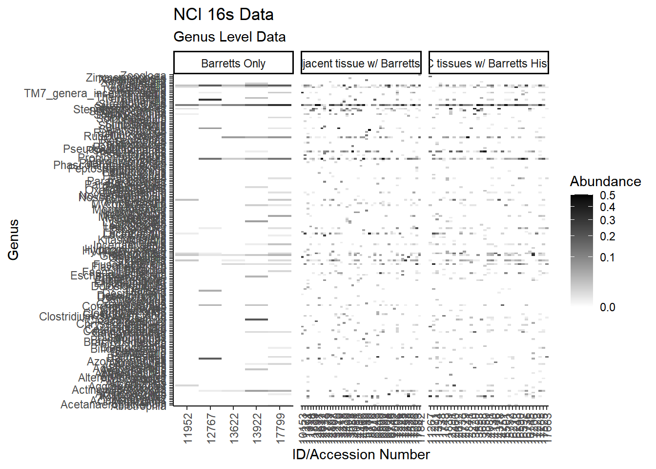
#ggsave("data/heatmap_nci16s_genus.pdf", p1, units="in", height=23, width=16)plot.dat <- dat.16s %>% filter(sample_type != "0") %>%
mutate(ID = as.factor(accession.number),
Genus = substr(Genus, 4, 1000),
Phylum = substr(Phylum, 4, 1000)) %>%
select(sample_type, Phylum, Genus, ID, Abundance)
plot.dat <- na.omit(plot.dat)
p1 <- ggplot(plot.dat, aes(x = ID, y = Phylum, fill = Abundance)) +
geom_tile()+
labs(title="NCI 16s Data", subtitle = "Phylum Level Data",
x = "ID/Accession Number") +
facet_grid(.~sample_type, scales="free")+
scale_fill_gradient(low="white", high="black", trans="sqrt", limits=c(0, 0.5)) +
theme_classic()+
theme(
axis.text.x = element_text(angle = 90, hjust = 1, vjust=0.5),
strip.text.y = element_text(angle = 0)
)
p1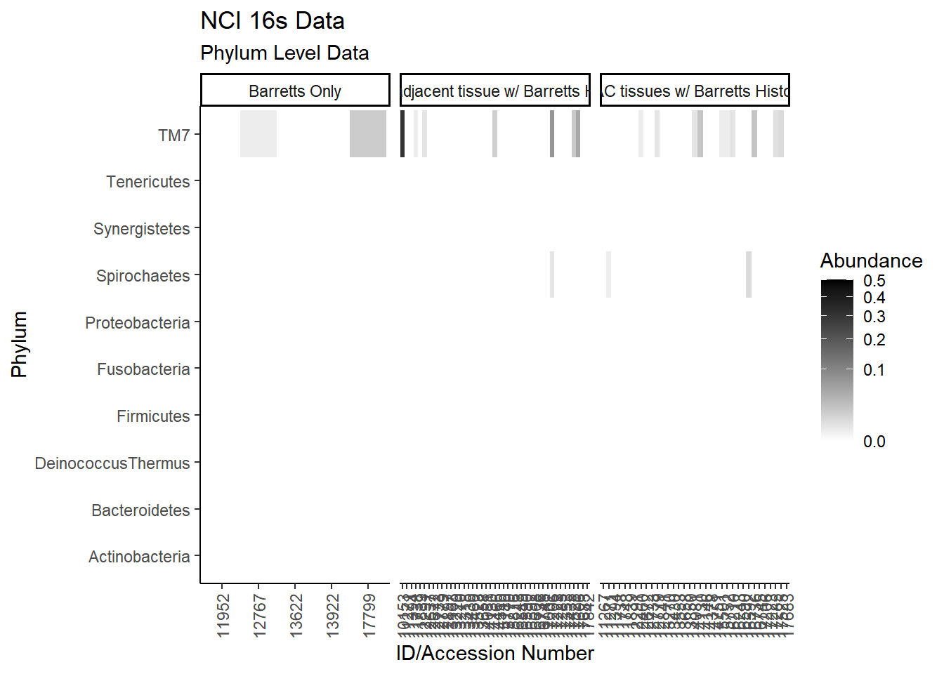
#ggsave("data/heatmap_nci16s_phylum.pdf", p1, units="in", height=10, width=16)plot.dat <- dat.rna %>% filter(sample_type != "0", Abundance > 0.001) %>%
select(sample_type, Phylum, Genus, Patient_ID, Abundance)
plot.dat <- na.omit(plot.dat)
p1 <- ggplot(plot.dat, aes(x = Patient_ID, y = Genus, fill = Abundance)) +
geom_tile()+
labs(title="TCGA RNAseq Data", subtitle = "Genus Level Data",
x = "ID/Accession Number") +
facet_grid(.~sample_type, scales="free")+
scale_fill_gradient(low="white", high="black", trans="sqrt", limits=c(0, 0.5)) +
theme_classic()+
theme(
axis.text.x = element_text(angle = 90, hjust = 1, vjust=0.5),
strip.text.y = element_text(angle = 0)
)
p1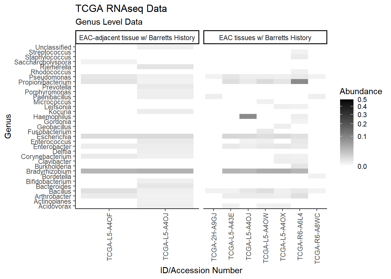
#ggsave("data/heatmap_tcgarna_genus.pdf", p1, units="in", height=23, width=16)plot.dat <- dat.rna %>% filter(sample_type != "0") %>%
select(sample_type, Phylum, Genus, Patient_ID, Abundance)
plot.dat <- na.omit(plot.dat)
p1 <- ggplot(plot.dat, aes(x = Patient_ID, y = Phylum, fill = Abundance)) +
geom_tile()+
labs(title="NCI 16s Data", subtitle = "Phylum Level Data",
x = "ID/Accession Number") +
facet_grid(.~sample_type, scales="free")+
scale_fill_gradient(low="white", high="black", trans="sqrt", limits=c(0, 0.5)) +
theme_classic()+
theme(
axis.text.x = element_text(angle = 90, hjust = 1, vjust=0.5),
strip.text.y = element_text(angle = 0)
)
p1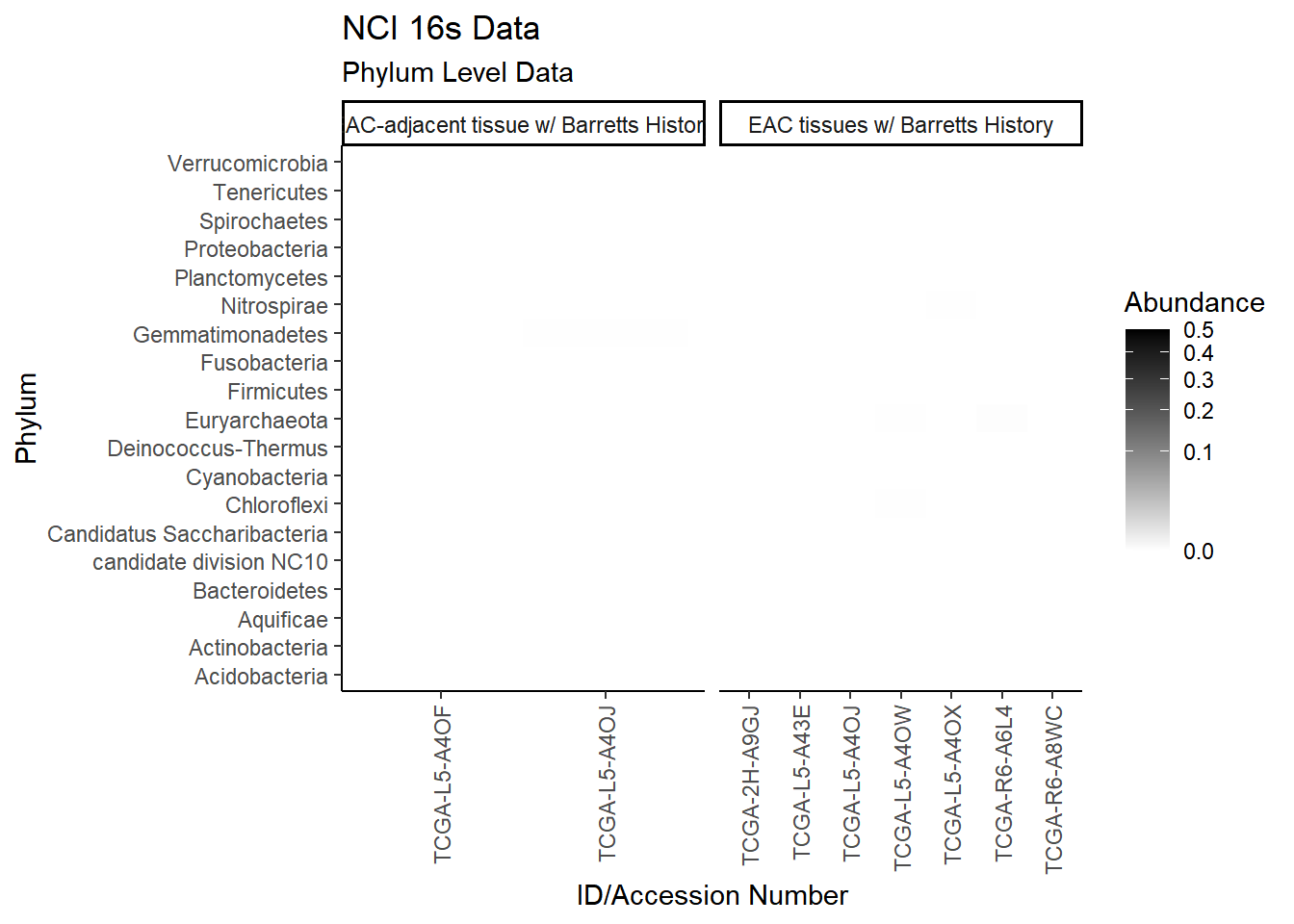
plot.dat <- dat.wgs %>% filter(sample_type != "0", Abundance > 0.001) %>%
  select(sample_type, Phylum, Genus, Patient_ID, Abundance)
plot.dat <- na.omit(plot.dat)

p1 <- ggplot(plot.dat, aes(x = Patient_ID, y = Genus, fill = Abundance)) +
  geom_tile()+
  labs(title="NCI 16s Data", subtitle = "Genus Level Data",
       x = "ID/Accession Number") +
  facet_grid(.~sample_type, scales="free")+
  scale_fill_gradient(low="white", high="black", trans="sqrt", limits=c(0, 0.5)) +
  theme_classic()+
  theme(
    axis.text.x = element_text(angle = 90, hjust = 1, vjust=0.5),
    strip.text.y = element_text(angle = 0)
  )
p1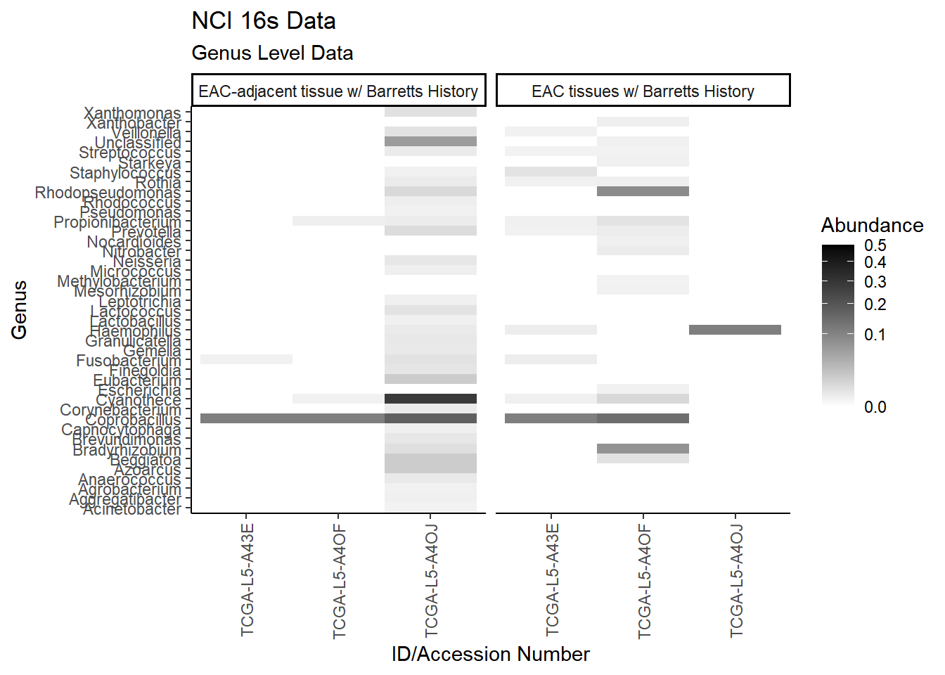
#ggsave("data/heatmap_nci16s_genus.pdf", p1, units="in", height=23, width=16)plot.dat <- dat.wgs %>% filter(sample_type != "0") %>%
select(sample_type, Phylum, Genus, Patient_ID, Abundance)
plot.dat <- na.omit(plot.dat)
p1 <- ggplot(plot.dat, aes(x = Patient_ID, y = Phylum, fill = Abundance)) +
geom_tile()+
labs(title="NCI 16s Data", subtitle = "Phylum Level Data",
x = "ID/Accession Number") +
facet_grid(.~sample_type, scales="free")+
scale_fill_gradient(low="white", high="black", trans="sqrt", limits=c(0, 0.5)) +
theme_classic()+
theme(
axis.text.x = element_text(angle = 90, hjust = 1, vjust=0.5),
strip.text.y = element_text(angle = 0)
)
p1
Specific OTUs
plot.dat <- dat.16s.s %>% filter(sample_type != "0") %>%
  mutate(ID = as.factor(accession.number),
         Genus = substr(Genus, 4, 1000),
         Phylum = substr(Phylum, 4, 1000)) %>%
  select(sample_type, Phylum, Genus, OTU, ID, Abundance)
plot.dat <- na.omit(plot.dat)

p1 <- ggplot(plot.dat, aes(x = ID, y = OTU, fill = Abundance)) +
  geom_tile()+
  labs(title="NCI 16s Data", y=NULL,
       x = "ID/Accession Number") +
  facet_grid(.~sample_type, scales="free")+
  scale_fill_gradient(low="white", high="black", trans="sqrt", limits=c(0, 0.5)) +
  theme_classic()+
  theme(
    axis.text.x = element_text(angle = 90, hjust = 1, vjust=0.5),
    strip.text.y = element_text(angle = 0)
  )
p1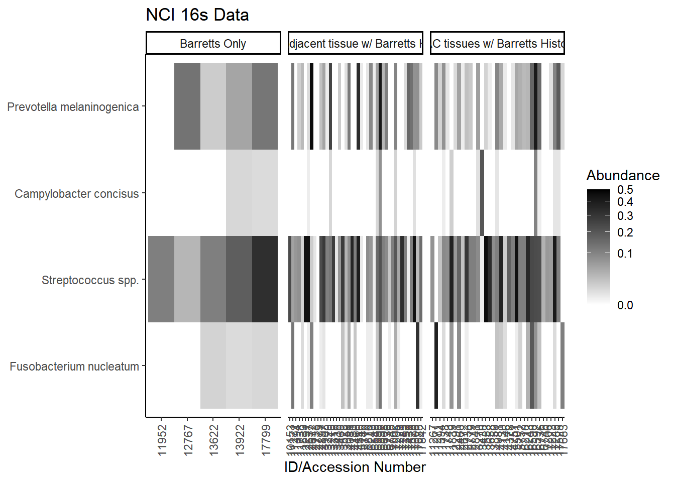
plot.dat <- dat.rna.s %>% filter(sample_type != "0", is.na(OTU1) == F) %>%
  select(sample_type, Phylum, Genus, OTU, Patient_ID, Abundance)
plot.dat <- na.omit(plot.dat)

p1 <- ggplot(plot.dat, aes(x = Patient_ID, y = OTU, fill = Abundance)) +
  geom_tile()+
  labs(title="TCGA RNAseq Data", y=NULL,
       x = "ID/Accession Number") +
  facet_grid(.~sample_type, scales="free")+
  scale_fill_gradient(low="white", high="black", trans="sqrt", limits=c(0, 0.5)) +
  theme_classic()+
  theme(
    axis.text.x = element_text(angle = 90, hjust = 1, vjust=0.5),
    strip.text.y = element_text(angle = 0)
  )
p1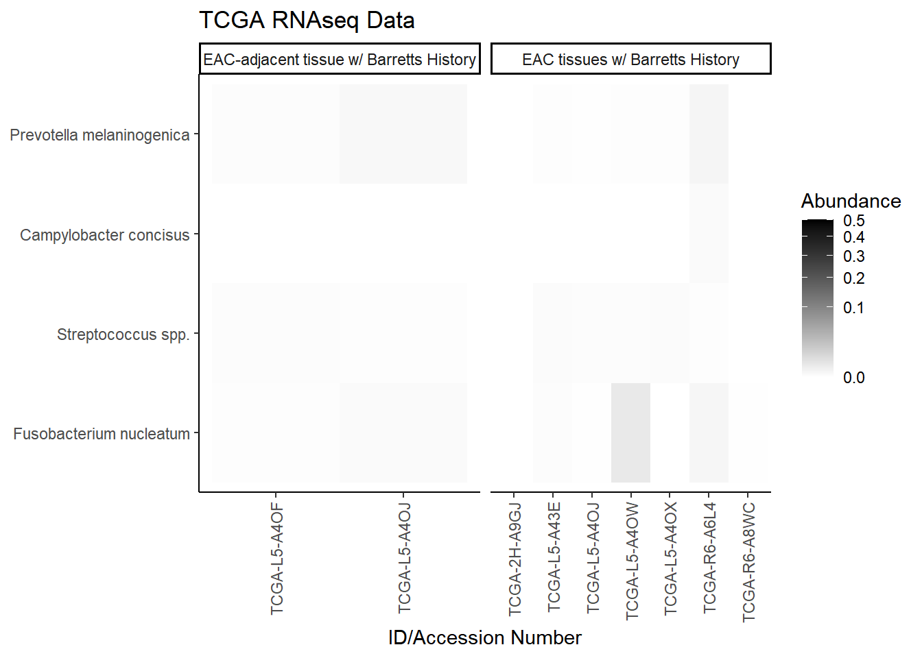
plot.dat <- dat.wgs.s %>% filter(sample_type != "0", is.na(OTU1) == F) %>%
  select(sample_type, Phylum, Genus, OTU, Patient_ID, Abundance)
plot.dat <- na.omit(plot.dat)

p1 <- ggplot(plot.dat, aes(x = Patient_ID, y = OTU, fill = Abundance)) +
  geom_tile()+
  labs(title="TCGA WGS Data", y=NULL,
       x = "ID/Accession Number") +
  facet_grid(.~sample_type, scales="free")+
  scale_fill_gradient(low="white", high="black", trans="sqrt", limits=c(0, 0.5)) +
  theme_classic()+
  theme(
    axis.text.x = element_text(angle = 90, hjust = 1, vjust=0.5),
    strip.text.y = element_text(angle = 0)
  )
p1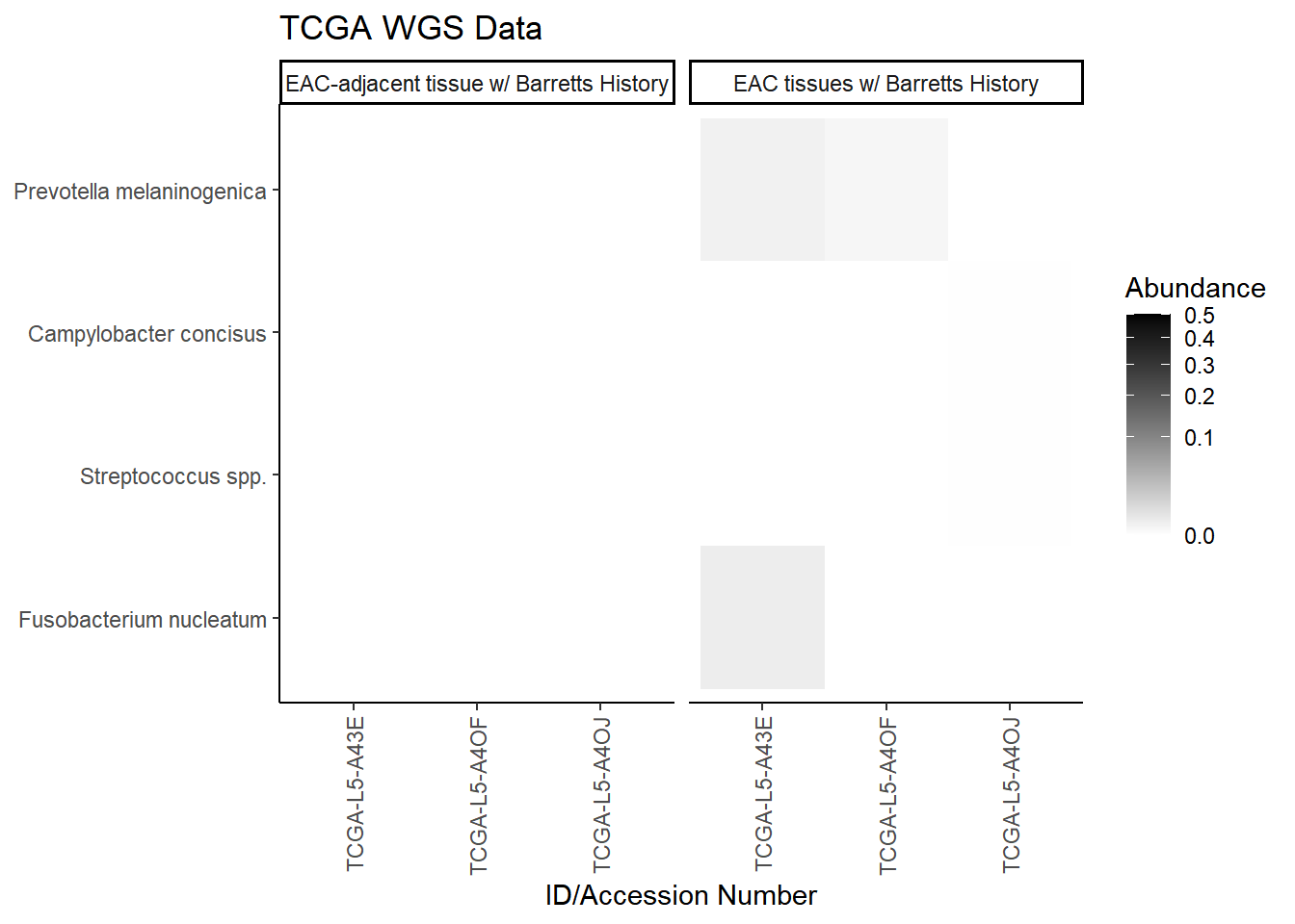
Stacked Bar Charts
All OTUs (RA > 0.001)
plot.dat <- dat.16s %>% filter(sample_type != "0", Abundance > 0.01 ) %>%
  mutate(ID = as.factor(accession.number),
         Genus = substr(Genus, 4, 1000),
         Phylum = substr(Phylum, 4, 1000))%>%
  dplyr::group_by(sample_type, Genus)%>%
  dplyr::summarise(
    Abundance = mean(Abundance, na.rm=T)
  )
`summarise()` regrouping output by 'sample_type' (override with `.groups` argument)p1 <- ggplot(plot.dat, aes(x=sample_type, y = Abundance, fill=Genus)) +
geom_bar(stat="identity")+
labs(title="NCI 16s Data",
subtitle = "Genus Level Data",
x = "Tissue Group",
y="Average Relative Abundance") +
theme_classic()+
theme(legend.position = "none")
p1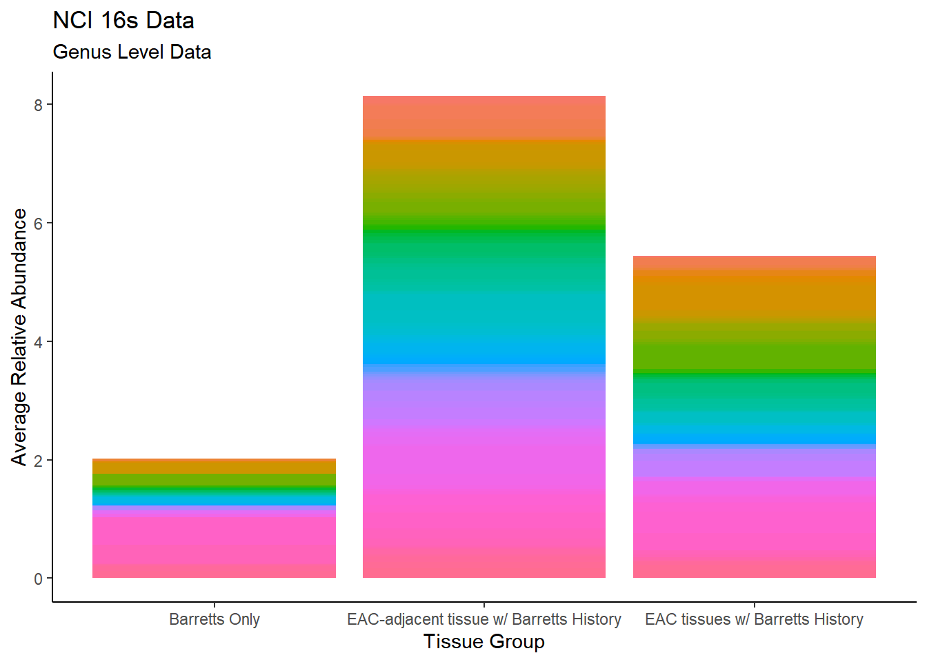
TOO MANY LEVELS FOR IT TO MAKE SENSE
plot.dat <- dat.16s %>% filter(sample_type != "0") %>%
  mutate(ID = as.factor(accession.number),
         Genus = substr(Genus, 4, 1000),
         Phylum = substr(Phylum, 4, 1000))%>%
  dplyr::group_by(sample_type, Phylum)%>%
  dplyr::summarise(
    Abundance = mean(Abundance, na.rm=T)
  )
`summarise()` regrouping output by 'sample_type' (override with `.groups` argument)p1 <- ggplot(plot.dat, aes(x=sample_type, y = Abundance, fill=Phylum)) +
geom_bar(stat="identity")+
labs(title="NCI 16s Data",
subtitle = "Phylum Level Data",
x = "Tissue Group",
y="Average Relative Abundance") +
theme_classic()
p1 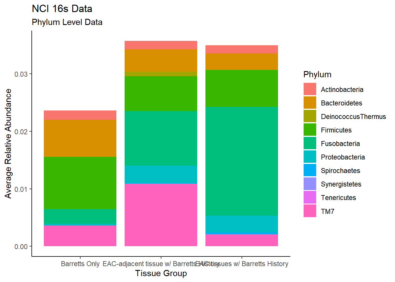
plot.dat <- dat.rna %>% filter(sample_type != "0", Abundance > 0.001)%>%
  dplyr::group_by(sample_type, Genus)%>%
  dplyr::summarise(
    Abundance = mean(Abundance, na.rm=T)
  )
`summarise()` regrouping output by 'sample_type' (override with `.groups` argument)p1 <- ggplot(plot.dat, aes(x=sample_type, y = Abundance, fill=Genus)) +
geom_bar(stat="identity")+
labs(title="TCGA RNAseq Data",
subtitle = "Genus Level Data",
x = "Tissue Group",
y="Average Relative Abundance") +
theme_classic()
p1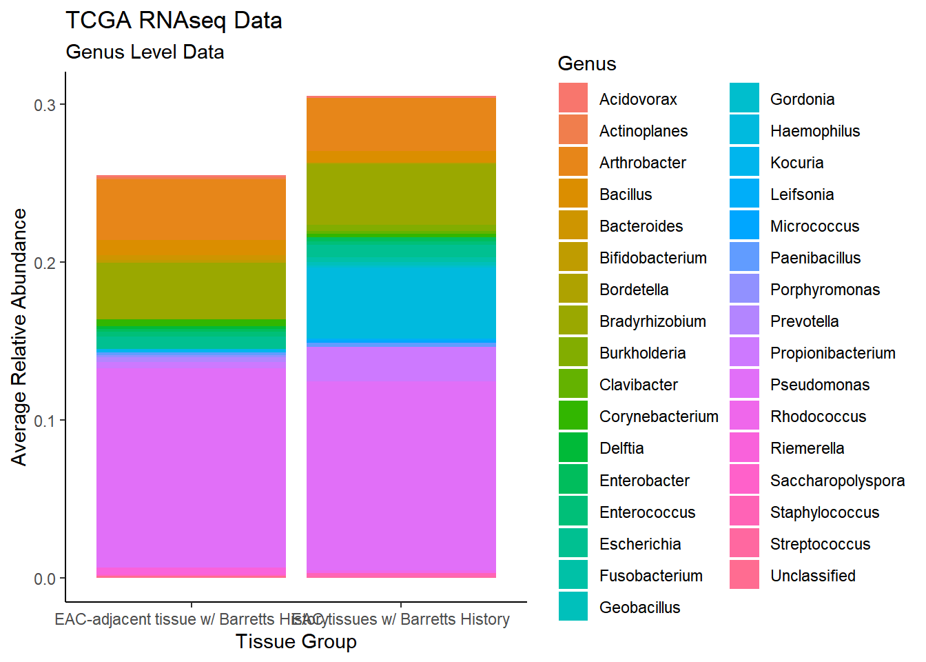
#ggsave("data/bar_tcgarna_genus.pdf", p1, units="in", height=23, width=16)plot.dat <- dat.rna %>% filter(sample_type != "0")%>%
dplyr::group_by(sample_type, Phylum)%>%
dplyr::summarise(
Abundance = mean(Abundance, na.rm=T)
)`summarise()` regrouping output by 'sample_type' (override with `.groups` argument)p1 <- ggplot(plot.dat, aes(x=sample_type, y = Abundance, fill=Phylum)) +
geom_bar(stat="identity")+
labs(title="TCGA RNAseq Data",
subtitle = "Phylum Level Data",
x = "Tissue Group",
y="Average Relative Abundance") +
theme_classic()
p1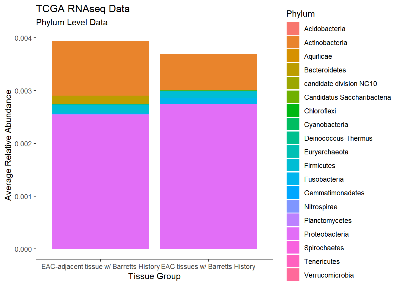
plot.dat <- dat.wgs %>% filter(sample_type != "0", Abundance > 0.001)%>%
  dplyr::group_by(sample_type, Genus)%>%
  dplyr::summarise(
    Abundance = mean(Abundance, na.rm=T)
  )
`summarise()` regrouping output by 'sample_type' (override with `.groups` argument)p1 <- ggplot(plot.dat, aes(x=sample_type, y = Abundance, fill=Genus)) +
geom_bar(stat="identity")+
labs(title="TCGA WGS Data",
subtitle = "Genus Level Data",
x = "Tissue Group",
y="Average Relative Abundance") +
theme_classic()
p1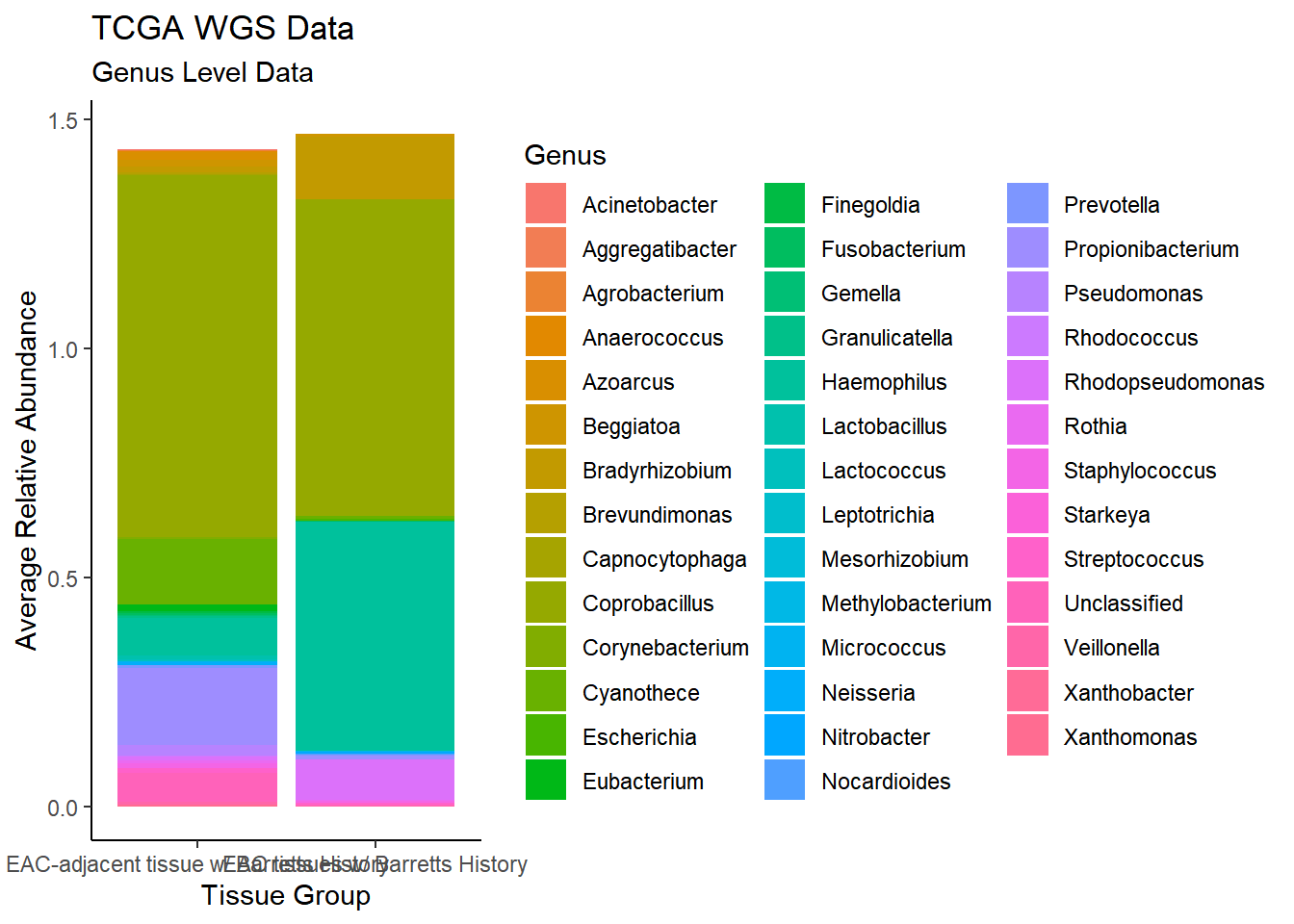
plot.dat <- dat.wgs %>% filter(sample_type != "0")%>%
  dplyr::group_by(sample_type, Phylum)%>%
  dplyr::summarise(
    Abundance = mean(Abundance, na.rm=T)
  )
`summarise()` regrouping output by 'sample_type' (override with `.groups` argument)p1 <- ggplot(plot.dat, aes(x=sample_type, y = Abundance, fill=Phylum)) +
geom_bar(stat="identity")+
labs(title="TCGA WGS Data",
subtitle = "Phylum Level Data",
x = "Tissue Group",
y="Average Relative Abundance") +
theme_classic()
p1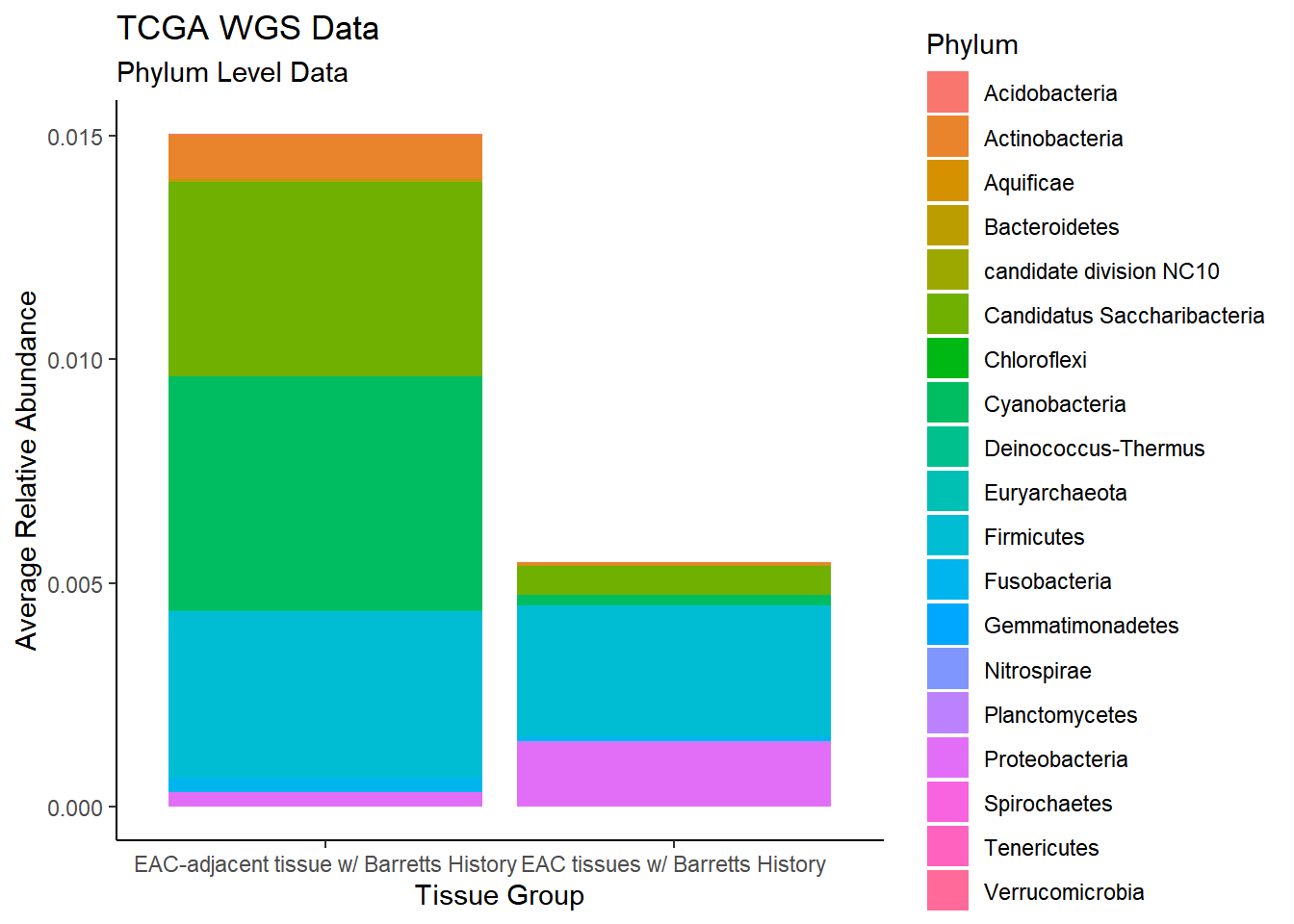
Specific OTUs
plot.dat <- dat.16s.s %>% filter(sample_type != "0") %>%
  mutate(ID = as.factor(accession.number),
         Genus = substr(Genus, 4, 1000),
         Phylum = substr(Phylum, 4, 1000))%>%
  dplyr::group_by(sample_type, OTU1)%>%
  dplyr::summarise(
    Abundance = mean(Abundance, na.rm=T)
  )
`summarise()` regrouping output by 'sample_type' (override with `.groups` argument)p1 <- ggplot(plot.dat, aes(x=sample_type, y = Abundance, fill=OTU1)) +
geom_bar(stat="identity")+
labs(title="NCI 16s Data",
x = "Tissue Group",
y="Average Relative Abundance") +
theme_classic()
p1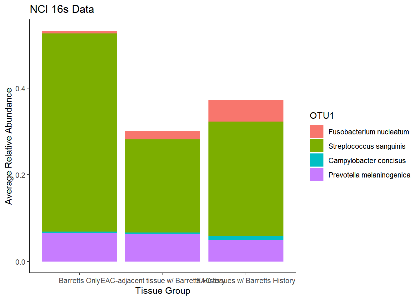
plot.dat <- dat.rna.s %>% filter(sample_type != "0", is.na(OTU1) == F)%>%
  dplyr::group_by(sample_type, OTU1)%>%
  dplyr::summarise(
    Abundance = mean(Abundance, na.rm=T)
  )
`summarise()` regrouping output by 'sample_type' (override with `.groups` argument)p1 <- ggplot(plot.dat, aes(x=sample_type, y = Abundance, fill=OTU1)) +
geom_bar(stat="identity")+
labs(title="NCI 16s Data",
x = "Tissue Group",
y="Average Relative Abundance") +
theme_classic()
p1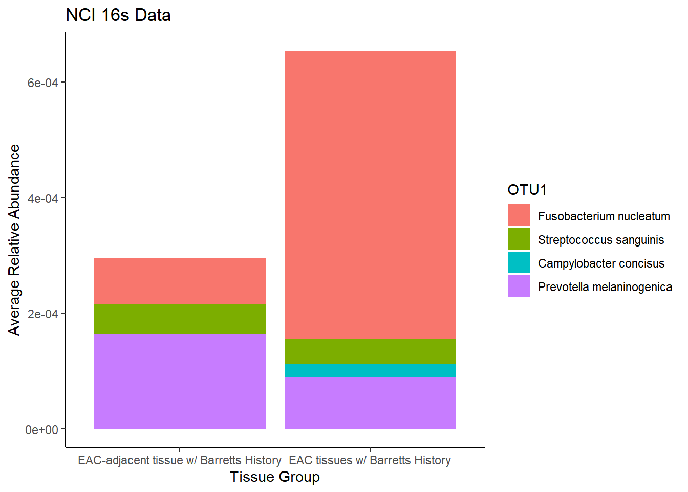
plot.dat <- dat.wgs.s %>% filter(sample_type != "0", is.na(OTU1) == F)%>%
  dplyr::group_by(sample_type, OTU1)%>%
  dplyr::summarise(
    Abundance = mean(Abundance, na.rm=T)
  )
`summarise()` regrouping output by 'sample_type' (override with `.groups` argument)p1 <- ggplot(plot.dat, aes(x=sample_type, y = Abundance, fill=OTU1)) +
geom_bar(stat="identity")+
labs(title="TCGA WGS Data",
x = "Tissue Group",
y="Average Relative Abundance") +
theme_classic()
p1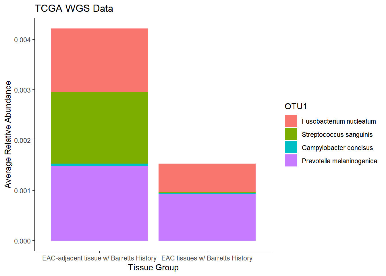
EAC Barretts to No Barretts Comparison
Heatmaps
All OTUs (RA > 0.001)
plot.dat <- dat.rna %>% filter(EACcomp != "0", Abundance > 0.001)

p1 <- ggplot(plot.dat, aes(x = Patient_ID, y = Genus, fill = Abundance)) +
  geom_tile()+
  labs(title="TCGA RNAseq Data", subtitle = "Genus Level Data",
       x = "ID/Accession Number") +
  facet_grid(.~EACcomp, scales="free")+
  scale_fill_gradient(low="white", high="black", trans="sqrt", limits=c(0, 0.5)) +
  theme_classic()+
  theme(
    axis.text.x = element_text(angle = 90, hjust = 1, vjust=0.5),
    strip.text.y = element_text(angle = 0)
  )
p1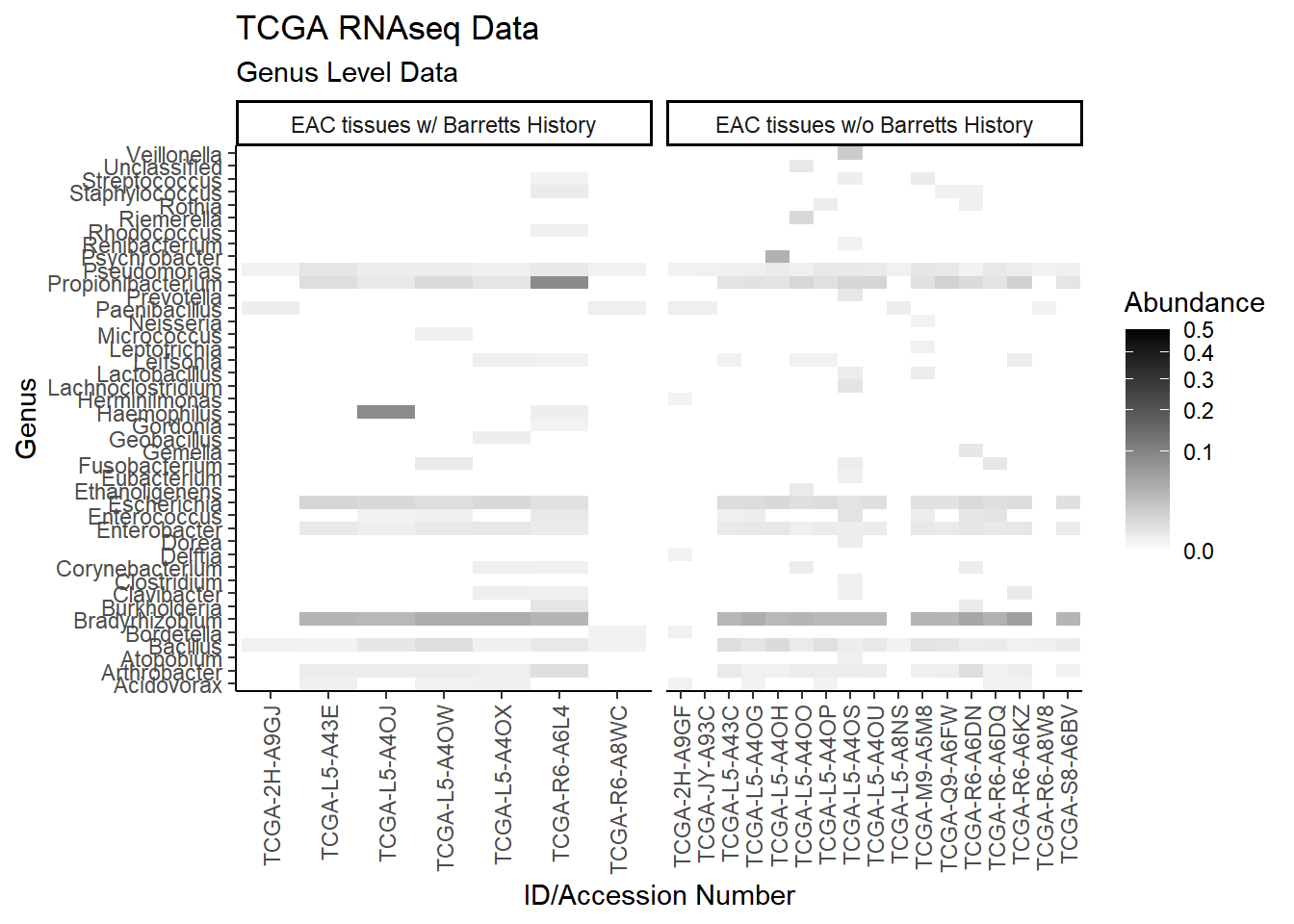
#ggsave("data/heatmap_tcgarna_genus.pdf", p1, units="in", height=23, width=16)plot.dat <- dat.rna %>% filter(EACcomp != "0") %>%
select(EACcomp, Phylum, Genus, Patient_ID, Abundance)
plot.dat <- na.omit(plot.dat)
p1 <- ggplot(plot.dat, aes(x = Patient_ID, y = Phylum, fill = Abundance)) +
geom_tile()+
labs(title="TCGA RNAseq Data", subtitle = "Phylum Level Data",
x = "ID/Accession Number") +
facet_grid(.~EACcomp, scales="free")+
scale_fill_gradient(low="white", high="black", trans="sqrt", limits=c(0, 0.001)) +
theme_classic()+
theme(
axis.text.x = element_text(angle = 90, hjust = 1, vjust=0.5),
strip.text.y = element_text(angle = 0)
)
p1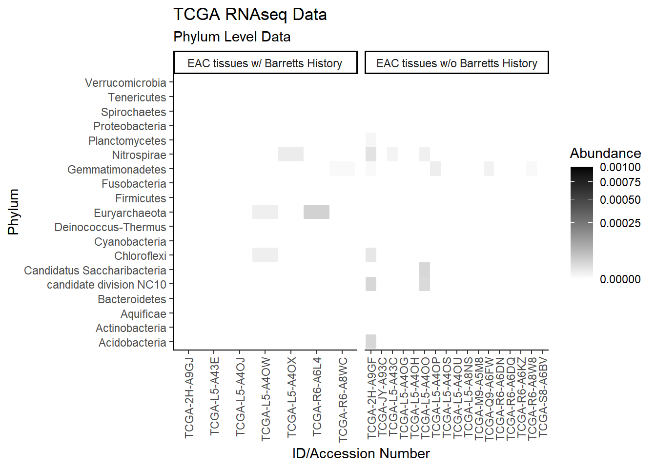
plot.dat <- dat.wgs %>% filter(EACcomp != "0", Abundance > 0.001) %>%
  select(EACcomp, Phylum, Genus, Patient_ID, Abundance)
plot.dat <- na.omit(plot.dat)

p1 <- ggplot(plot.dat, aes(x = Patient_ID, y = Genus, fill = Abundance)) +
  geom_tile()+
  labs(title="TCGA WGS Data", subtitle = "Genus Level Data",
       x = "ID/Accession Number") +
  facet_grid(.~EACcomp, scales="free")+
  scale_fill_gradient(low="white", high="black", trans="sqrt", limits=c(0, 0.5)) +
  theme_classic()+
  theme(
    axis.text.x = element_text(angle = 90, hjust = 1, vjust=0.5),
    strip.text.y = element_text(angle = 0)
  )
p1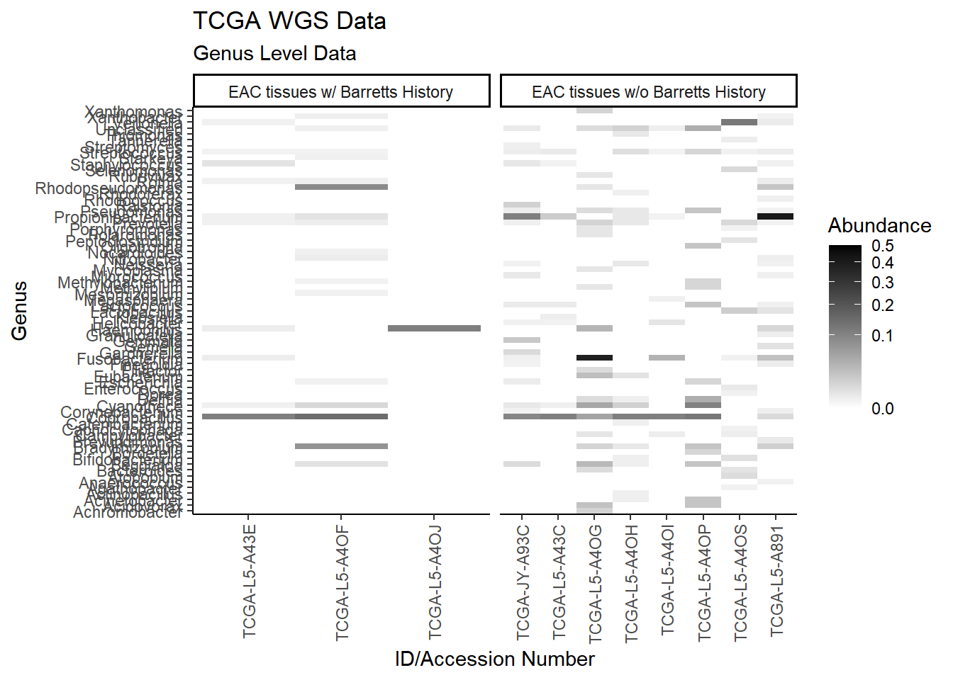
plot.dat <- dat.wgs %>% filter(EACcomp != "0") %>%
  select(EACcomp, Phylum, Genus, Patient_ID, Abundance)
plot.dat <- na.omit(plot.dat)

p1 <- ggplot(plot.dat, aes(x = Patient_ID, y = Phylum, fill = Abundance)) +
  geom_tile()+
  labs(title="TCGA WGS Data", subtitle = "Phylum Level Data",
       x = "ID/Accession Number") +
  facet_grid(.~EACcomp, scales="free")+
  scale_fill_gradient(low="white", high="black", trans="sqrt", limits=c(0, 0.001)) +
  theme_classic()+
  theme(
    axis.text.x = element_text(angle = 90, hjust = 1, vjust=0.5),
    strip.text.y = element_text(angle = 0)
  )
p1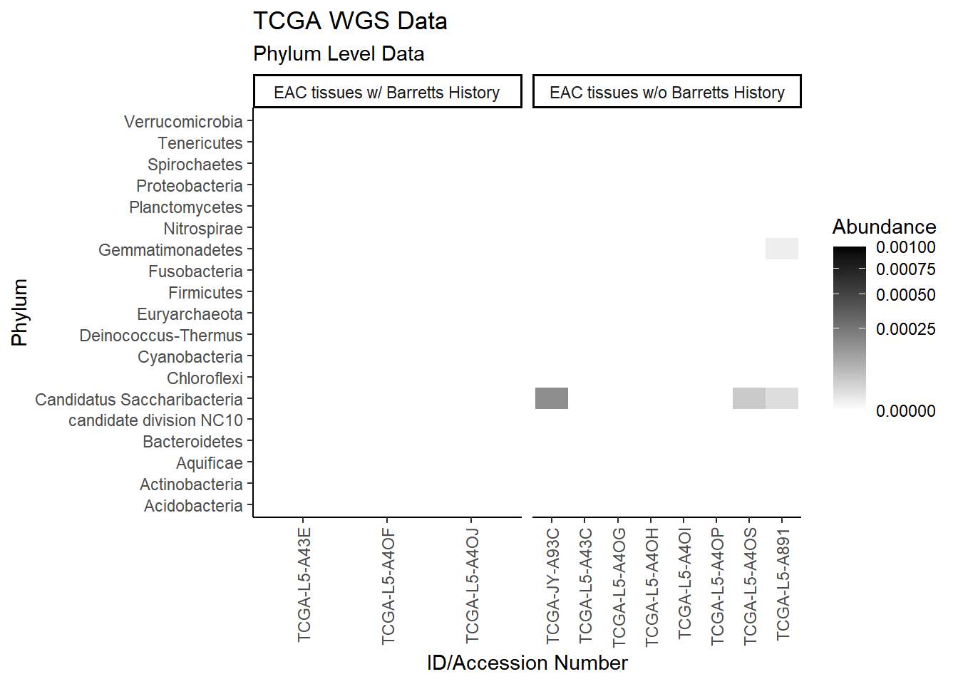
Specific OTUs
plot.dat <- dat.rna.s %>% filter(EACcomp != "0", is.na(OTU1) == F) %>%
  select(EACcomp, OTU1, Patient_ID, Abundance)
plot.dat <- na.omit(plot.dat)

p1 <- ggplot(plot.dat, aes(x = Patient_ID, y = OTU1, fill = Abundance)) +
  geom_tile()+
  labs(title="TCGA RNAseq Data", y=NULL,
       x = "ID/Accession Number") +
  facet_grid(.~EACcomp, scales="free")+
  scale_fill_gradient(low="white", high="black", trans="sqrt", limits=c(0, 0.1)) +
  theme_classic()+
  theme(
    axis.text.x = element_text(angle = 90, hjust = 1, vjust=0.5),
    strip.text.y = element_text(angle = 0)
  )
p1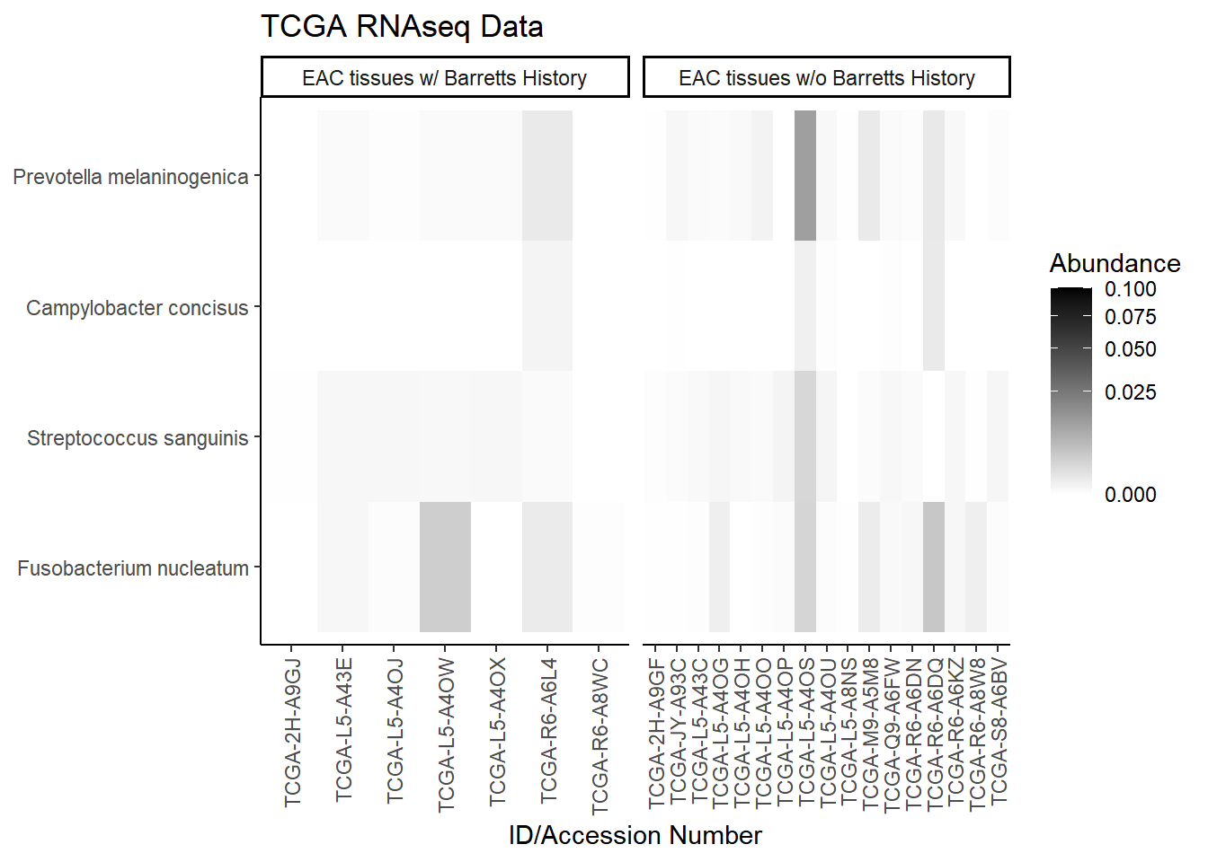
plot.dat <- dat.wgs.s %>% filter(EACcomp != "0", is.na(OTU1) == F) %>%
  select(EACcomp, OTU1, Patient_ID, Abundance)
plot.dat <- na.omit(plot.dat)


p1 <- ggplot(plot.dat, aes(x =Patient_ID, y = OTU1, fill = Abundance)) +
  geom_tile()+
  labs(title="TCGA WGS Data", y=NULL,
       x = "ID/Accession Number") +
  facet_grid(.~EACcomp, scales="free")+
  scale_fill_gradient(low="white", high="black", trans="sqrt", limits=c(0, 0.5)) +
  theme_classic()+
  theme(
    axis.text.x = element_text(angle = 90, hjust = 1, vjust=0.5),
    strip.text.y = element_text(angle = 0)
  )
p1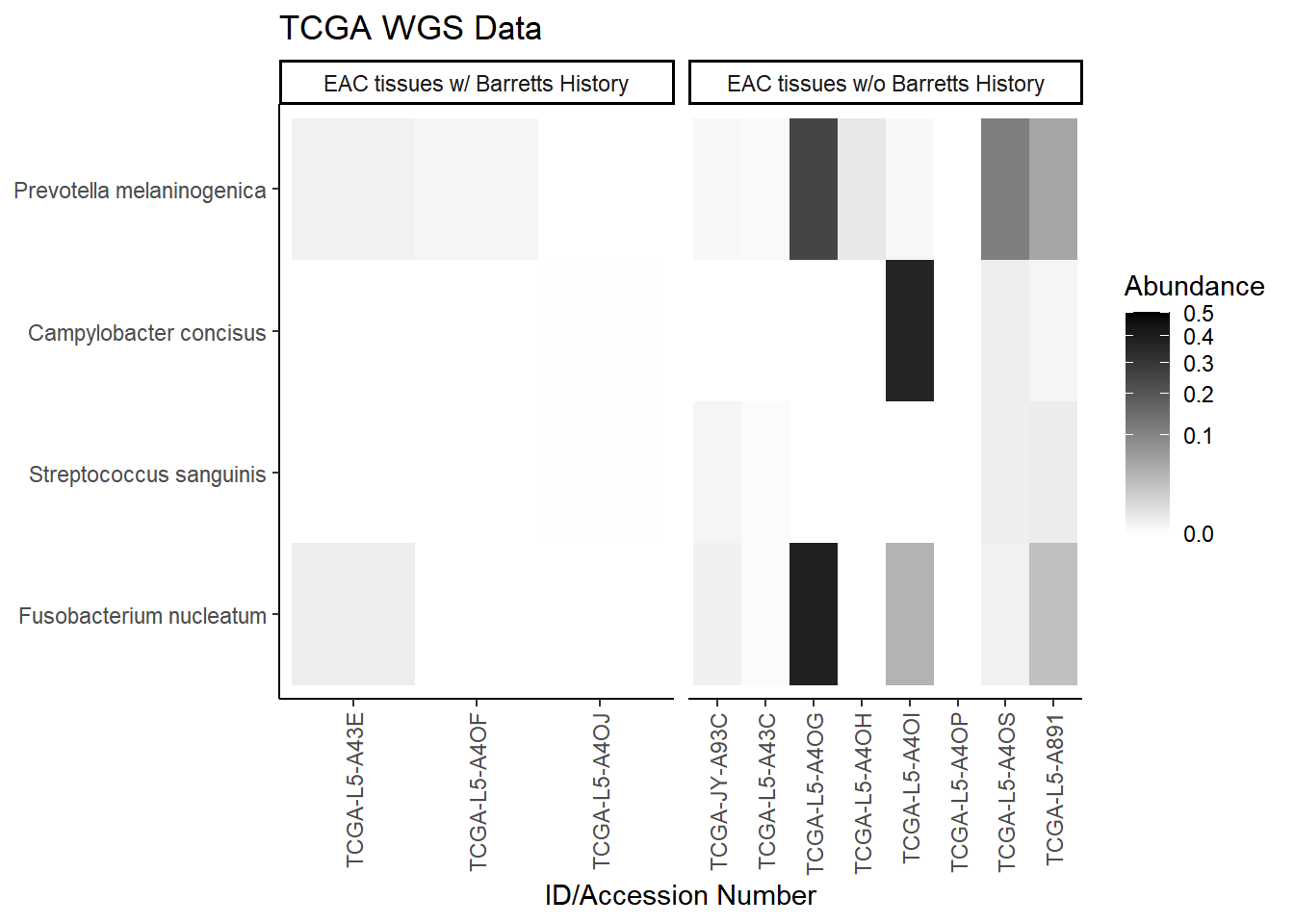
Stacked Bar Charts
All OTUs (RA > 0.001)
plot.dat <- dat.rna %>% filter(EACcomp != "0", Abundance > 0.001)%>%
  dplyr::group_by(EACcomp, Genus)%>%
  dplyr::summarise(
    Abundance = mean(Abundance, na.rm=T)
  )
`summarise()` regrouping output by 'EACcomp' (override with `.groups` argument)p1 <- ggplot(plot.dat, aes(x=EACcomp, y = Abundance, fill=Genus)) +
geom_bar(stat="identity")+
labs(title="TCGA RNAseq Data",
subtitle = "Genus Level Data",
x = "Tissue Group",
y="Average Relative Abundance") +
theme_classic()
p1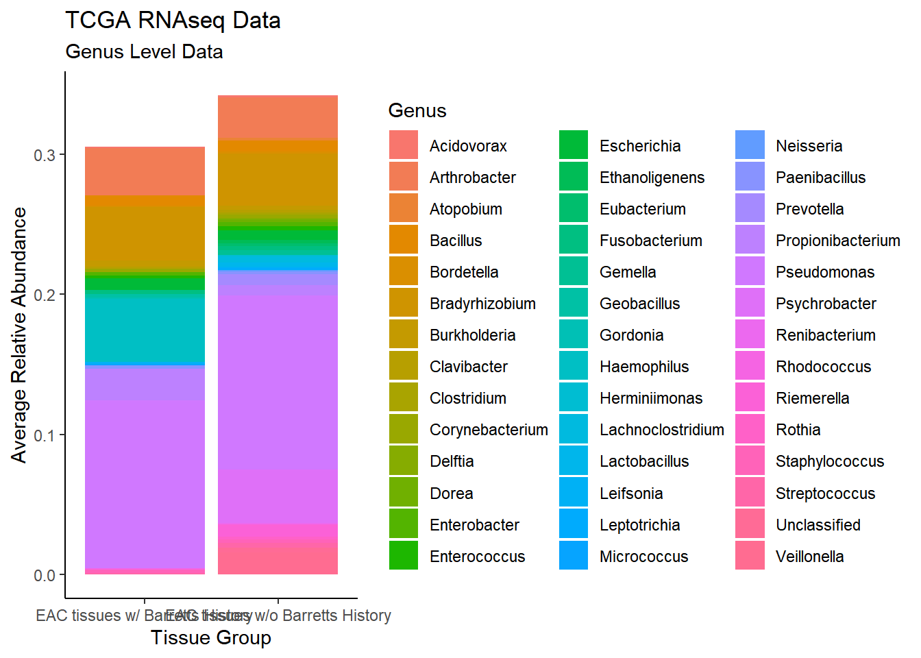
#ggsave("data/bar_tcgarna_genus.pdf", p1, units="in", height=23, width=16)plot.dat <- dat.rna %>% filter(EACcomp != "0")%>%
dplyr::group_by(EACcomp, Phylum)%>%
dplyr::summarise(
Abundance = mean(Abundance, na.rm=T)
)`summarise()` regrouping output by 'EACcomp' (override with `.groups` argument)p1 <- ggplot(plot.dat, aes(x=EACcomp, y = Abundance, fill=Phylum)) +
geom_bar(stat="identity")+
labs(title="TCGA RNAseq Data",
subtitle = "Phylum Level Data",
x = "Tissue Group",
y="Average Relative Abundance") +
theme_classic()
p1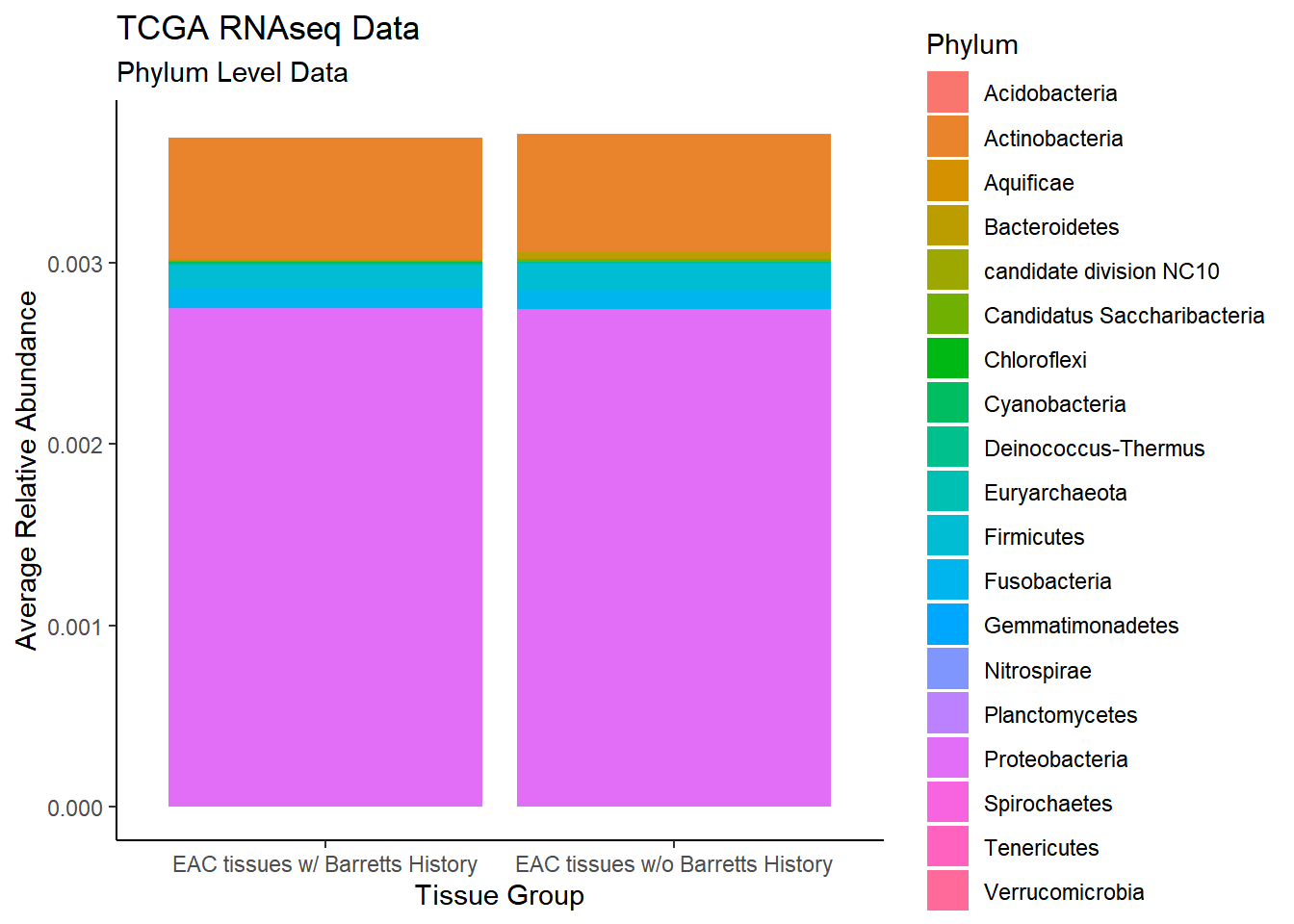
plot.dat <- dat.wgs %>% filter(EACcomp != "0", Abundance > 0.001)%>%
  dplyr::group_by(EACcomp, Genus)%>%
  dplyr::summarise(
    Abundance = mean(Abundance, na.rm=T)
  )
`summarise()` regrouping output by 'EACcomp' (override with `.groups` argument)p1 <- ggplot(plot.dat, aes(x=EACcomp, y = Abundance, fill=Genus)) +
geom_bar(stat="identity")+
labs(title="TCGA WGS Data",
subtitle = "Genus Level Data",
x = "Tissue Group",
y="Average Relative Abundance") +
theme_classic()
p1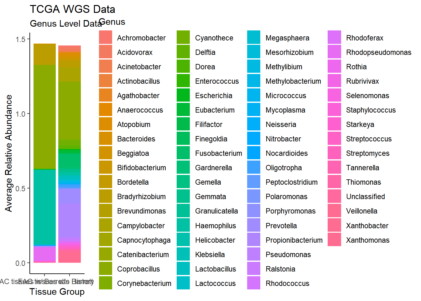
plot.dat <- dat.wgs %>% filter(EACcomp != "0")%>%
  dplyr::group_by(EACcomp, Phylum)%>%
  dplyr::summarise(
    Abundance = mean(Abundance, na.rm=T)
  )
`summarise()` regrouping output by 'EACcomp' (override with `.groups` argument)p1 <- ggplot(plot.dat, aes(x=EACcomp, y = Abundance, fill=Phylum)) +
geom_bar(stat="identity")+
labs(title="TCGA WGS Data",
subtitle = "Phylum Level Data",
x = "Tissue Group",
y="Average Relative Abundance") +
theme_classic()
p1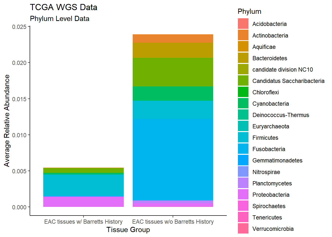
Specific OTUs
plot.dat <- dat.rna.s %>% filter(EACcomp != "0", is.na(OTU1) == F)%>%
  dplyr::group_by(EACcomp, OTU1)%>%
  dplyr::summarise(
    Abundance = mean(Abundance, na.rm=T)
  )
`summarise()` regrouping output by 'EACcomp' (override with `.groups` argument)p1 <- ggplot(plot.dat, aes(x=EACcomp, y = Abundance, fill=OTU1)) +
geom_bar(stat="identity")+
labs(title="TCGA RNA seq Data",
x = "Tissue Group",
y="Average Relative Abundance") +
theme_classic()
p1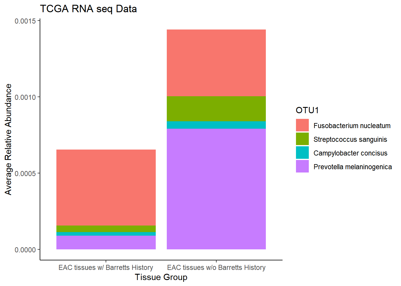
plot.dat <- dat.wgs.s %>% filter(EACcomp != "0", is.na(OTU1) == F)%>%
  dplyr::group_by(EACcomp, OTU1)%>%
  dplyr::summarise(
    Abundance = mean(Abundance, na.rm=T)
  )
`summarise()` regrouping output by 'EACcomp' (override with `.groups` argument)p1 <- ggplot(plot.dat, aes(x=EACcomp, y = Abundance, fill=OTU1)) +
geom_bar(stat="identity")+
labs(title="TCGA WGS Data",
x = "Tissue Group",
y="Average Relative Abundance") +
theme_classic()
p1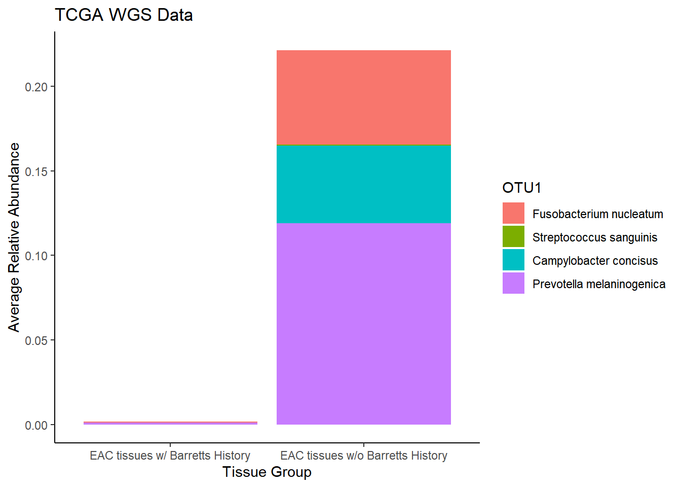
sessionInfo()R version 4.0.2 (2020-06-22)
Platform: x86_64-w64-mingw32/x64 (64-bit)
Running under: Windows 10 x64 (build 18363)
Matrix products: default
locale:
[1] LC_COLLATE=English_United States.1252
[2] LC_CTYPE=English_United States.1252
[3] LC_MONETARY=English_United States.1252
[4] LC_NUMERIC=C
[5] LC_TIME=English_United States.1252
attached base packages:
[1] stats graphics grDevices utils datasets methods base
other attached packages:
[1] car_3.0-8 carData_3.0-4 gvlma_1.0.0.3 patchwork_1.0.1
[5] viridis_0.5.1 viridisLite_0.3.0 gridExtra_2.3 xtable_1.8-4
[9] kableExtra_1.1.0 plyr_1.8.6 data.table_1.13.0 readxl_1.3.1
[13] forcats_0.5.0 stringr_1.4.0 dplyr_1.0.1 purrr_0.3.4
[17] readr_1.3.1 tidyr_1.1.1 tibble_3.0.3 ggplot2_3.3.2
[21] tidyverse_1.3.0 lmerTest_3.1-2 lme4_1.1-23 Matrix_1.2-18
[25] vegan_2.5-6 lattice_0.20-41 permute_0.9-5 phyloseq_1.32.0
[29] workflowr_1.6.2
loaded via a namespace (and not attached):
[1] minqa_1.2.4 colorspace_1.4-1 rio_0.5.16
[4] ellipsis_0.3.1 rprojroot_1.3-2 XVector_0.28.0
[7] fs_1.5.0 rstudioapi_0.11 farver_2.0.3
[10] fansi_0.4.1 lubridate_1.7.9 xml2_1.3.2
[13] codetools_0.2-16 splines_4.0.2 knitr_1.29
[16] ade4_1.7-15 jsonlite_1.7.0 nloptr_1.2.2.2
[19] broom_0.7.0 cluster_2.1.0 dbplyr_1.4.4
[22] BiocManager_1.30.10 compiler_4.0.2 httr_1.4.2
[25] backports_1.1.7 assertthat_0.2.1 cli_2.0.2
[28] later_1.1.0.1 htmltools_0.5.0 tools_4.0.2
[31] igraph_1.2.5 gtable_0.3.0 glue_1.4.1
[34] reshape2_1.4.4 Rcpp_1.0.5 Biobase_2.48.0
[37] cellranger_1.1.0 vctrs_0.3.2 Biostrings_2.56.0
[40] multtest_2.44.0 ape_5.4 nlme_3.1-148
[43] iterators_1.0.12 xfun_0.19 openxlsx_4.1.5
[46] rvest_0.3.6 lifecycle_0.2.0 statmod_1.4.34
[49] zlibbioc_1.34.0 MASS_7.3-51.6 scales_1.1.1
[52] hms_0.5.3 promises_1.1.1 parallel_4.0.2
[55] biomformat_1.16.0 rhdf5_2.32.2 curl_4.3
[58] yaml_2.2.1 stringi_1.4.6 S4Vectors_0.26.1
[61] foreach_1.5.0 BiocGenerics_0.34.0 zip_2.0.4
[64] boot_1.3-25 rlang_0.4.7 pkgconfig_2.0.3
[67] evaluate_0.14 Rhdf5lib_1.10.1 labeling_0.3
[70] tidyselect_1.1.0 magrittr_1.5 R6_2.4.1
[73] IRanges_2.22.2 generics_0.0.2 DBI_1.1.0
[76] foreign_0.8-80 pillar_1.4.6 haven_2.3.1
[79] withr_2.2.0 mgcv_1.8-31 abind_1.4-5
[82] survival_3.2-3 modelr_0.1.8 crayon_1.3.4
[85] rmarkdown_2.5 grid_4.0.2 blob_1.2.1
[88] git2r_0.27.1 reprex_0.3.0 digest_0.6.25
[91] webshot_0.5.2 httpuv_1.5.4 numDeriv_2016.8-1.1
[94] stats4_4.0.2 munsell_0.5.0