Disease investigated by ancestry
Last updated: 2022-02-17
Checks: 7 0
Knit directory: genomics_ancest_disease_dispar/
This reproducible R Markdown analysis was created with workflowr (version 1.6.2). The Checks tab describes the reproducibility checks that were applied when the results were created. The Past versions tab lists the development history.
Great! Since the R Markdown file has been committed to the Git repository, you know the exact version of the code that produced these results.
Great job! The global environment was empty. Objects defined in the global environment can affect the analysis in your R Markdown file in unknown ways. For reproduciblity it’s best to always run the code in an empty environment.
The command set.seed(20220216) was run prior to running the code in the R Markdown file. Setting a seed ensures that any results that rely on randomness, e.g. subsampling or permutations, are reproducible.
Great job! Recording the operating system, R version, and package versions is critical for reproducibility.
Nice! There were no cached chunks for this analysis, so you can be confident that you successfully produced the results during this run.
Great job! Using relative paths to the files within your workflowr project makes it easier to run your code on other machines.
Great! You are using Git for version control. Tracking code development and connecting the code version to the results is critical for reproducibility.
The results in this page were generated with repository version 7347b5d. See the Past versions tab to see a history of the changes made to the R Markdown and HTML files.
Note that you need to be careful to ensure that all relevant files for the analysis have been committed to Git prior to generating the results (you can use wflow_publish or wflow_git_commit). workflowr only checks the R Markdown file, but you know if there are other scripts or data files that it depends on. Below is the status of the Git repository when the results were generated:
Ignored files:
    Ignored:    data/gwas_catalog/

Untracked files:
    Untracked:  data/cdc/

Unstaged changes:
    Modified:   README.md
Note that any generated files, e.g. HTML, png, CSS, etc., are not included in this status report because it is ok for generated content to have uncommitted changes.
These are the previous versions of the repository in which changes were made to the R Markdown (analysis/disease_inves_by_ancest.Rmd) and HTML (docs/disease_inves_by_ancest.html) files. If you’ve configured a remote Git repository (see ?wflow_git_remote), click on the hyperlinks in the table below to view the files as they were in that past version.
| File | Version | Author | Date | Message |
|---|---|---|---|---|
| Rmd | 7347b5d | Isobel Beasley | 2022-02-17 | Add initial plotting using gwas cat stats |
library(dplyr)
library(ggplot2)

gwas_study_info = data.table::fread("data/gwas_catalog/gwas-catalog-v1.0.3-studies-r2022-02-02.tsv",
                                    sep = "\t",
                                    quote = "")

gwas_ancest_info = data.table::fread("./data/gwas_catalog/gwas_catalog-ancestry_r2022-02-02.tsv",
                                     sep = "\t",
                                     quote = "")

# Set up custom theme for ggplots
custom_theme <-
  list(
    theme_bw() +
      theme(
        panel.border = element_blank(),
        axis.line = element_line(),
        text = element_text(size = 16),
        legend.position = "bottom",
        strip.background = element_blank(),
        axis.text.x = element_text(angle = 90, hjust = 1, vjust = 0.5)
      )
  )
Plot figure Martin et al. 2019 like
For all ancestries
# code adapted from https://github.com/armartin/prs_disparities/blob/master/gwas_disparities_time.R

# Order GWAS catalog by date
gwas_ancest_info <- gwas_ancest_info %>% arrange(DATE)

# calculate cumulative number of individuals
gwas_ancest_info = gwas_ancest_info %>%
                   mutate(cum_num = cumsum(ifelse(is.na(`NUMBER OF INDIVDUALS`), 0, `NUMBER OF INDIVDUALS`)))


# plot cumulative numbers
gwas_ancest_info %>%
  group_by(DATE) %>%
  slice_max(`NUMBER OF INDIVDUALS`) %>%
  ggplot(aes(x=DATE,y=cum_num/1e6)) +
  geom_line() +
  #geom_area(position = 'stack') +
  scale_x_date(date_labels = '%Y', date_breaks = "2 years") +
  custom_theme +
  labs(x = "Year", y = "Individuals in GWAS catalog (millons)")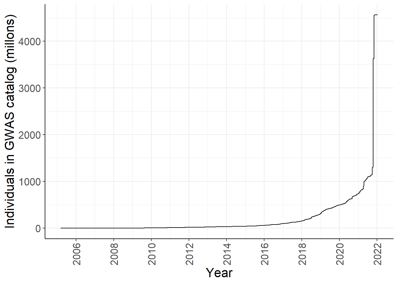
Group ancestry into broader categories
grouped_ancest = vector()

for(study_ancest in unique(gwas_ancest_info$`BROAD ANCESTRAL CATEGORY`)){

    if(study_ancest %in% c('Sub-Saharan African, African American or Afro-Caribbean',
                           'Sub-Saharan African, African unspecified',
                           'African-American or Afro-Caribbean')){


      grouped_ancest = append(grouped_ancest,'African')


    } else if(study_ancest %in% c('East Asian, Asian unspecified',
                                  'South Asian, East Asian ',
                                  'South Asian, South East Asian',
                                  'South Asian, South East Asian, East Asian',
                                   'South East Asian, East Asian',
                                  'South East Asian, South Asian, East Asian')) {


      grouped_ancest = append(grouped_ancest,'Asian unspecified')


    } else if(study_ancest == 'Greater Middle Eastern (Middle Eastern, North African or Persian)') {


      grouped_ancest = append(grouped_ancest,'Middle Eastern')


    } else if(study_ancest %in% c('Aboriginal Australian', 'Oceanian')) {


      grouped_ancest = append(grouped_ancest,'Oceanic')


    } else if(grepl(", ", study_ancest)) {


      grouped_ancest = append(grouped_ancest,'Multiple')


    } else if(study_ancest %in% "Hispanic or Latin American"){


      grouped_ancest = append(grouped_ancest,'Hispanic/Latin American')


     } else {

      grouped_ancest = append(grouped_ancest,study_ancest)
    }


  }


ancest_group = data.frame(group_ancest = grouped_ancest,
                         `BROAD ANCESTRAL CATEGORY` = unique(gwas_ancest_info$`BROAD ANCESTRAL CATEGORY`))

gwas_ancest_info = inner_join(
            gwas_ancest_info %>% mutate(BROAD.ANCESTRAL.CATEGORY = `BROAD ANCESTRAL CATEGORY`),
            ancest_group)
Joining, by = "BROAD.ANCESTRAL.CATEGORY"gwas_ancest_info %>%
group_by(group_ancest) %>%
summarise(n = sum(`NUMBER OF INDIVDUALS`, na.rm = TRUE))# A tibble: 18 x 2
group_ancest n
<chr> <dbl>
1 African 60441
2 African American or Afro-Caribbean 8278986
3 African unspecified 3028217
4 Asian unspecified 4697042
5 Central Asian 42945
6 East Asian 124056468
7 European 4235129752
8 Hispanic/Latin American 10840275
9 Middle Eastern 348192
10 Multiple 56292255
11 Native American 91973
12 NR 110448036
13 Oceanic 116432
14 Other 194359
15 Other admixed ancestry 107563
16 South Asian 6138158
17 South East Asian 170602
18 Sub-Saharan African 827401gwas_ancest_info %>%
group_by(group_ancest) %>%
mutate(ancest_cumsum = cumsum(`NUMBER OF INDIVDUALS`)) %>%
ggplot(aes(x=DATE,y=ancest_cumsum/(10^6), fill = group_ancest)) +
#geom_area() +
geom_area() +
scale_x_date(date_labels = '%Y', date_breaks = "2 years") +
theme_classic() +
labs(x = "Year", y = "Individuals in GWAS catalog (millons)") +
scale_fill_brewer(palette = "Set1")Warning: Removed 32641 rows containing missing values (position_stack).Warning in RColorBrewer::brewer.pal(n, pal): n too large, allowed maximum for palette Set1 is 9
Returning the palette you asked for with that many colors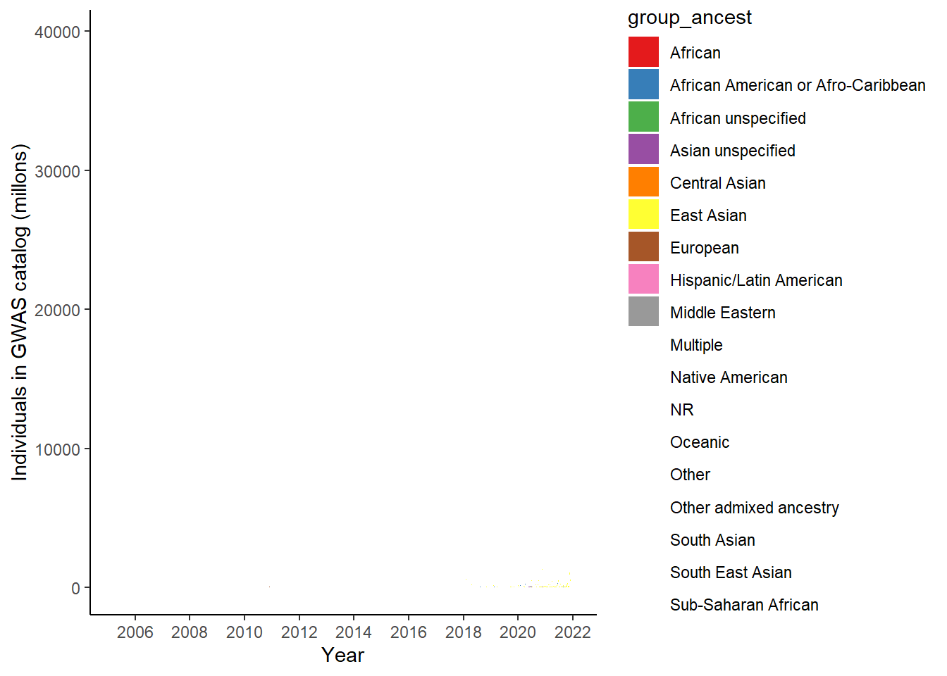
inner_join(
           gwas_study_info %>% select(`STUDY ACCESSION`, `DISEASE/TRAIT`, `MAPPED_TRAIT`),
           gwas_ancest_info %>% select(`STUDY ACCESSION`, `NUMBER OF INDIVDUALS`, `BROAD ANCESTRAL CATEGORY`)) %>%
  group_by(`BROAD ANCESTRAL CATEGORY`, `DISEASE/TRAIT`) %>%
  summarise(n = sum(`NUMBER OF INDIVDUALS`)) %>%
  group_by(`BROAD ANCESTRAL CATEGORY`) %>%
  slice_max(n,n = 5)
Joining, by = "STUDY ACCESSION"`summarise()` has grouped output by 'BROAD ANCESTRAL CATEGORY'. You can override using the `.groups` argument.# A tibble: 802 x 3
# Groups: BROAD ANCESTRAL CATEGORY [192]
`BROAD ANCESTRAL CATEGORY` `DISEASE/TRAIT` n
<chr> <chr> <int>
1 Aboriginal Australian Urinary albumin-to-creatin~ 746
2 Aboriginal Australian Otitis media 391
3 Aboriginal Australian Type 2 diabetes 391
4 Aboriginal Australian Body mass index 361
5 African American or Afro-Caribbean Cataracts 262576
6 African American or Afro-Caribbean Body mass index 228346
7 African American or Afro-Caribbean Type 2 diabetes 202731
8 African American or Afro-Caribbean Diastolic blood pressure 200474
9 African American or Afro-Caribbean Systolic blood pressure 200474
10 African American or Afro-Caribbean, Afric~ Type 2 diabetes 287510
# ... with 792 more rowsDisease statistics CDC
cdc_stats = data.table::fread("data/cdc/Underlying Cause of Death, 1999-2020.txt",
                              drop = c("Notes", "Race Code", "Cause of death Code")) %>%
             filter(!if_any(everything(), ~.x == ""))

cdc_stats %>%
  group_by(Race) %>%
  slice_max(Deaths,n=10)
# A tibble: 40 x 6
# Groups: Race [4]
Race `Cause of death` Deaths Population `Crude Rate` `Age Adjusted R~
<chr> <chr> <int> <int64> <chr> <chr>
1 America~ Atherosclerotic hea~ 15927 88362592 18.0 33.9
2 America~ Bronchus or lung, u~ 15334 88362592 17.4 28.3
3 America~ Acute myocardial in~ 13755 88362592 15.6 26.7
4 America~ Chronic obstructive~ 10500 88362592 11.9 22.0
5 America~ Atherosclerotic car~ 9090 88362592 10.3 16.7
6 America~ Unspecified diabete~ 8307 88362592 9.4 15.0
7 America~ Alcoholic cirrhosis~ 8129 88362592 9.2 10.7
8 America~ Stroke, not specifi~ 6055 88362592 6.9 13.8
9 America~ Pneumonia, unspecif~ 5728 88362592 6.5 12.5
10 America~ Unspecified dementia 5092 88362592 5.8 13.9
# ... with 30 more rows
sessionInfo()R version 4.1.0 (2021-05-18)
Platform: x86_64-w64-mingw32/x64 (64-bit)
Running under: Windows 10 x64 (build 19043)
Matrix products: default
locale:
[1] LC_COLLATE=English_Australia.1252 LC_CTYPE=English_Australia.1252
[3] LC_MONETARY=English_Australia.1252 LC_NUMERIC=C
[5] LC_TIME=English_Australia.1252
attached base packages:
[1] stats graphics grDevices utils datasets methods base
other attached packages:
[1] ggplot2_3.3.5 dplyr_1.0.6 workflowr_1.6.2
loaded via a namespace (and not attached):
[1] Rcpp_1.0.6 RColorBrewer_1.1-2 highr_0.9 pillar_1.6.1
[5] compiler_4.1.0 bslib_0.2.5.1 later_1.2.0 jquerylib_0.1.4
[9] git2r_0.29.0 tools_4.1.0 bit_4.0.4 digest_0.6.27
[13] gtable_0.3.0 jsonlite_1.7.2 evaluate_0.14 lifecycle_1.0.0
[17] tibble_3.1.2 pkgconfig_2.0.3 rlang_0.4.11 rstudioapi_0.13
[21] cli_3.1.0 DBI_1.1.1 yaml_2.2.1 xfun_0.24
[25] withr_2.4.2 stringr_1.4.0 knitr_1.33 generics_0.1.0
[29] fs_1.5.0 vctrs_0.3.8 sass_0.4.0 bit64_4.0.5
[33] grid_4.1.0 rprojroot_2.0.2 tidyselect_1.1.1 data.table_1.14.0
[37] glue_1.4.2 R6_2.5.0 fansi_0.4.2 rmarkdown_2.9
[41] farver_2.1.0 purrr_0.3.4 magrittr_2.0.1 whisker_0.4
[45] scales_1.1.1 promises_1.2.0.1 ellipsis_0.3.2 htmltools_0.5.1.1
[49] assertthat_0.2.1 colorspace_2.0-1 httpuv_1.6.1 labeling_0.4.2
[53] utf8_1.2.1 stringi_1.6.1 munsell_0.5.0 crayon_1.4.1