Fetching iCite Metrics for GWAS Catalog Publications
Isobel Beasley
Last updated: 2025-08-21
Checks: 7 0
Knit directory:
genomics_ancest_disease_dispar/
This reproducible R Markdown analysis was created with workflowr (version 1.7.1). The Checks tab describes the reproducibility checks that were applied when the results were created. The Past versions tab lists the development history.
Great! Since the R Markdown file has been committed to the Git repository, you know the exact version of the code that produced these results.
Great job! The global environment was empty. Objects defined in the global environment can affect the analysis in your R Markdown file in unknown ways. For reproduciblity it’s best to always run the code in an empty environment.
The command set.seed(20220216) was run prior to running
the code in the R Markdown file. Setting a seed ensures that any results
that rely on randomness, e.g. subsampling or permutations, are
reproducible.
Great job! Recording the operating system, R version, and package versions is critical for reproducibility.
Nice! There were no cached chunks for this analysis, so you can be confident that you successfully produced the results during this run.
Great job! Using relative paths to the files within your workflowr project makes it easier to run your code on other machines.
Great! You are using Git for version control. Tracking code development and connecting the code version to the results is critical for reproducibility.
The results in this page were generated with repository version 605013e. See the Past versions tab to see a history of the changes made to the R Markdown and HTML files.
Note that you need to be careful to ensure that all relevant files for
the analysis have been committed to Git prior to generating the results
(you can use wflow_publish or
wflow_git_commit). workflowr only checks the R Markdown
file, but you know if there are other scripts or data files that it
depends on. Below is the status of the Git repository when the results
were generated:
Ignored files:
    Ignored:    .Rproj.user/
    Ignored:    data/gwas_catalog/
    Ignored:    output/gwas_study_info_cohort_corrected.csv

Untracked files:
    Untracked:  data/.DS_Store
    Untracked:  renv/

Unstaged changes:
    Modified:   .Rprofile
    Modified:   code/collapse_diseases.R
Note that any generated files, e.g. HTML, png, CSS, etc., are not included in this status report because it is ok for generated content to have uncommitted changes.
These are the previous versions of the repository in which changes were
made to the R Markdown (analysis/icite_rcr.Rmd) and HTML
(docs/icite_rcr.html) files. If you’ve configured a remote
Git repository (see ?wflow_git_remote), click on the
hyperlinks in the table below to view the files as they were in that
past version.
| File | Version | Author | Date | Message |
|---|---|---|---|---|
| Rmd | d0edbb8 | IJbeasley | 2025-08-06 | Halfway through converting cohorts |
| html | 88e1648 | IJbeasley | 2025-08-05 | Build site. |
| Rmd | 852dd98 | IJbeasley | 2025-08-05 | Convert icite analysis to workflowr page |
knitr::opts_chunk$set(
  echo = TRUE,
  message = FALSE,
  warning = FALSE
)
library(httr)
library(jsonlite)
library(dplyr)
library(data.table)
library(purrr)
library(ggplot2)
Overview
- Retrieves citation metrics from NIH’s iCite API for publications listed in the GWAS Catalog (like in Reales & Wallace, 2023 - sharing gwas data results in more citations)
- Due to iCite API limitations, PMIDs of papers in the GWAS catalog are queried in chunks.
- Note: tried iciteR R package (as I believe Reales & Wallace do) but found it didn’t retrieve the complete set of metrics - I think because adding &format=csv to api call seems to cause problems example call: iCiteR::get_metrics(“27599104”)
1. Define Function to Query iCite API
Define a helper function that accepts a chunk of PMIDs and returns a data frame with citation data.
# Function to fetch a chunk of PMIDs from the iCite API
fetch_icite_chunk <- function(pmid_chunk) {
  pmid_vec <- paste0(pmid_chunk, collapse = ",")

  # Construct API URL
  url <- paste0("https://icite.od.nih.gov/api/pubs?pmids=",
                pmid_vec)

  # Perform GET request
  response <- GET(url)

  # Parse the response content as JSON
  data_list <- fromJSON(content(response, "text"), flatten = TRUE)

  # Convert to data frame
  pub_df <- as.data.frame(data_list)

  # Remove "data." prefix from column names
  pub_df <- pub_df |> rename_all(~gsub("data.", "", .x))

  # Drop large nested citation data (optional)
  pub_df <- pub_df |> select(-c(citedByPmidsByYear))

  return(pub_df)
}
2. Load and Clean GWAS Catalog Study Data
Extract unique PMIDs for papers from the GWAS catalog
# Load GWAS Catalog studies
gwas_study_info <- fread("data/gwas_catalog/gwas-catalog-v1.0.3.1-studies-r2025-07-21.tsv",
                         sep = "\t", quote = "")

# Standardize column names (remove spaces)
gwas_study_info <- gwas_study_info |> rename_all(~gsub(" ", "_", .x))

# Extract unique publication information
gwas_study_info <- gwas_study_info |>
  select(FIRST_AUTHOR, DATE, JOURNAL, PUBMED_ID) |>
  distinct()

# Vector of PMIDs
pmid <- gwas_study_info$PUBMED_ID
3. Fetch Citation Metrics from iCite
To comply with iCite rate limits, we split the PMIDs into batches (≤ 400 per request) and apply our fetch function.
# Split PMIDs into chunks of 400
pmid_chunks <- split(pmid, ceiling(seq_along(pmid) / 400))

# Fetch citation metrics for all chunks
all_results <- map_dfr(pmid_chunks, fetch_icite_chunk)
Confirm RCR calculations match provided equation
# Check if RCR ≈ citations_per_year / expected_citations_per_year
check = all_results |>
  select(field_citation_rate,
         expected_citations_per_year,
         citations_per_year,
         relative_citation_ratio) |>
  mutate(calculated_rcr = citations_per_year / expected_citations_per_year)

head(check)
field_citation_rate expected_citations_per_year citations_per_year
1 7.254935 2.838550 5.000000
2 7.241446 2.834556 3.428571
3 8.243854 3.116852 38.000000
4 8.075742 3.131311 87.083333
5 8.682365 3.545011 6.000000
6 8.981703 3.644344 45.200000
relative_citation_ratio calculated_rcr
1 1.761462 1.761462
2 1.209562 1.209562
3 12.191789 12.191789
4 27.810498 27.810498
5 1.692519 1.692519
6 12.402780 12.402780check = check |>
filter(!is.na(relative_citation_ratio))
sum(check$calculated_rcr == check$relative_citation_ratio)[1] 7012nrow(check)[1] 7012Visual exploration of data
4. Distribution of citation metrics
# Example: Distribution of Relative Citation Ratios (RCR)
ggplot(all_results, aes(x = relative_citation_ratio)) +
  geom_histogram(bins = 50) +
  theme_minimal() +
  labs(title = "Distribution of RCR among GWAS publications",
       x = "Relative Citation Ratio (RCR)",
       y = "Count")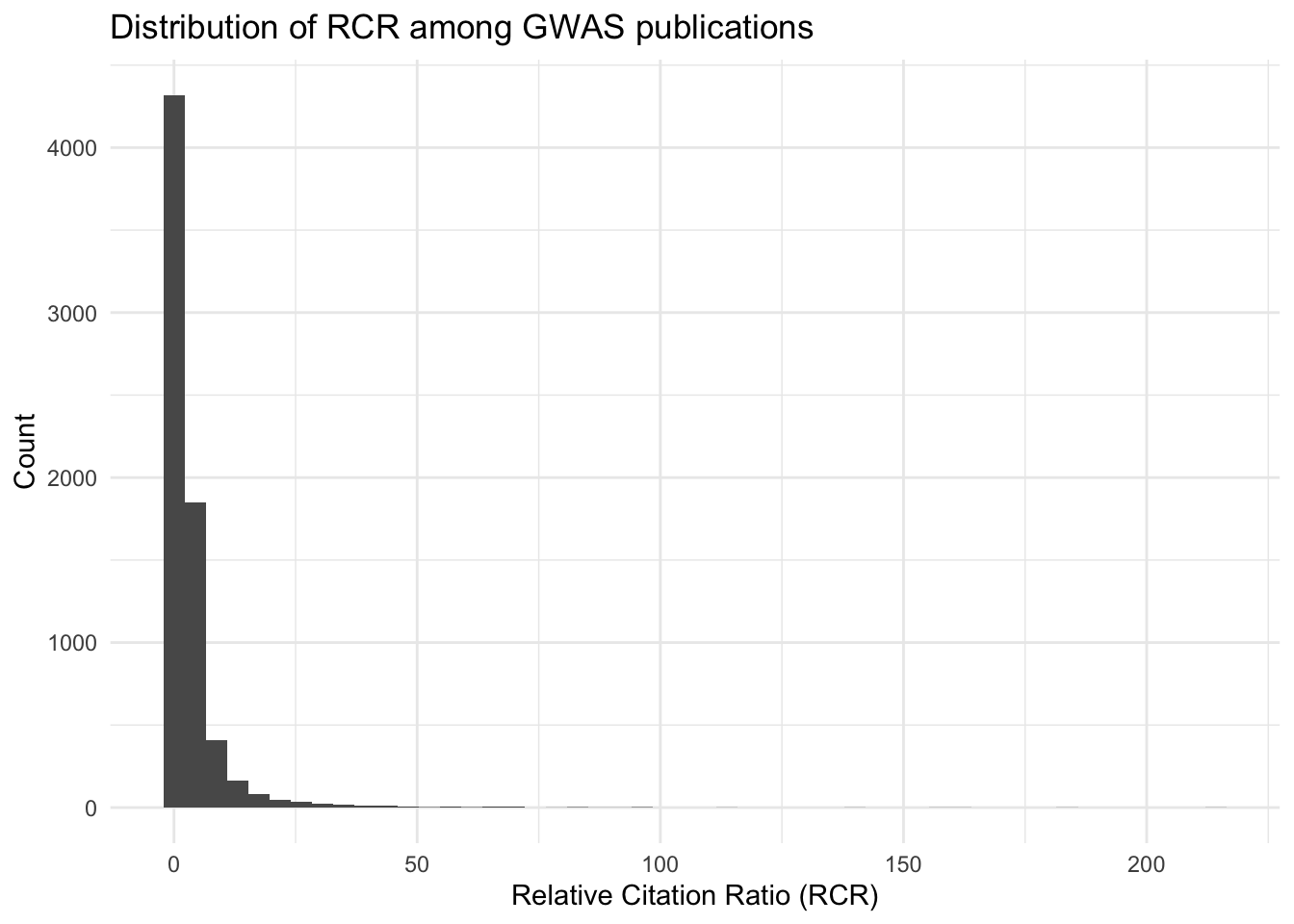
| Version | Author | Date |
|---|---|---|
| 88e1648 | IJbeasley | 2025-08-05 |
# Summary of citation counts
summary(all_results$relative_citation_ratio)
Min. 1st Qu. Median Mean 3rd Qu. Max. NA's
0.0000 0.7022 1.5072 3.6552 3.4473 214.2744 313 # Distribution of raw citation counts
ggplot(all_results, aes(x = citation_count)) +
geom_histogram() +
theme_bw() +
labs(title = "Distribution of Raw Citation Counts among GWAS catalog publications")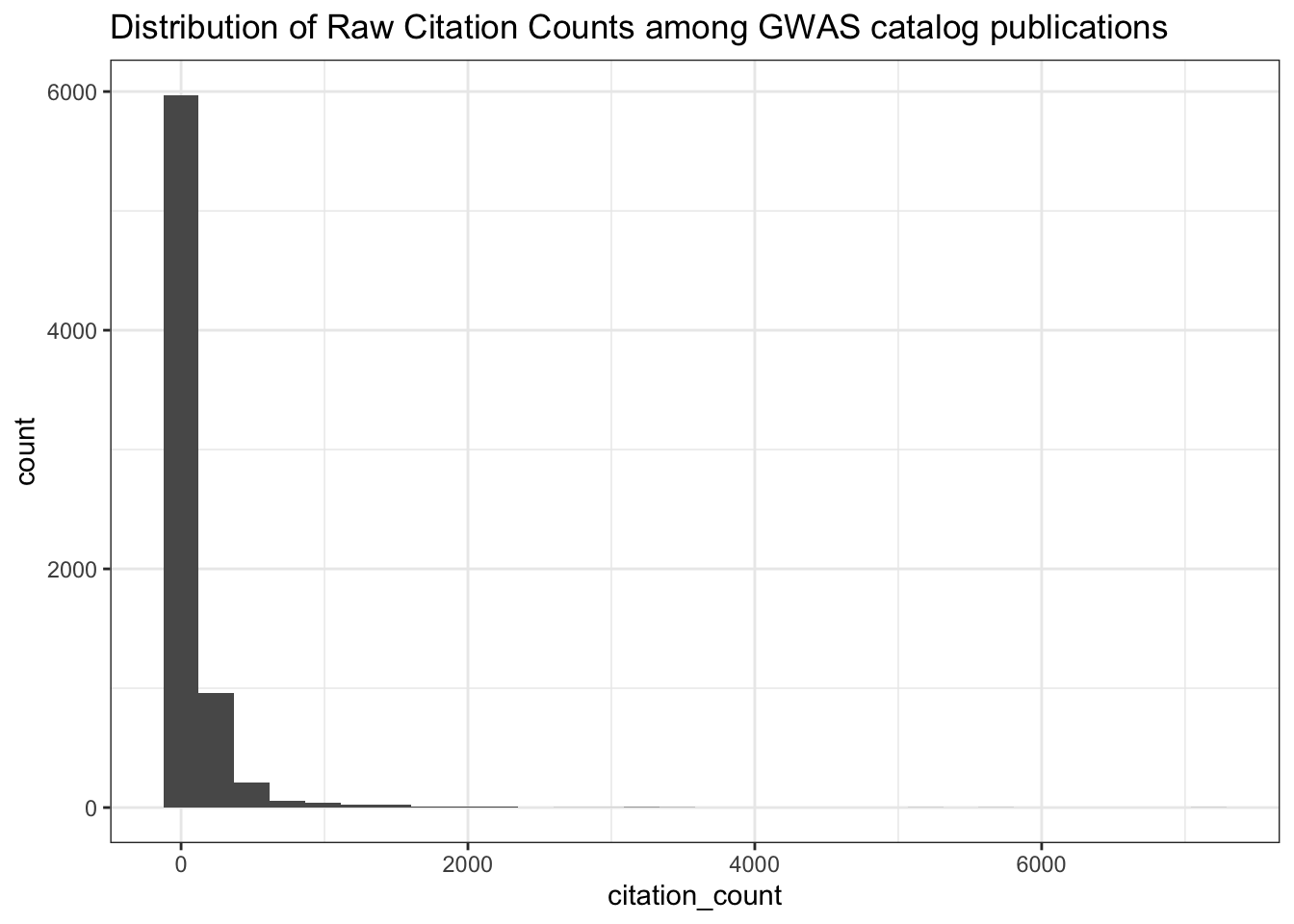
| Version | Author | Date |
|---|---|---|
| 88e1648 | IJbeasley | 2025-08-05 |
# Summary of citation counts
summary(all_results$citation_count)
Min. 1st Qu. Median Mean 3rd Qu. Max.
0.00 11.00 30.00 98.85 88.00 7167.00 5. Investigate Missing and Zero RCRs
# Publication Year of Papers with NA RCR
all_results |>
  filter(is.na(relative_citation_ratio)) |>
  ggplot(aes(x = year)) +
  geom_histogram() +
  scale_x_continuous(breaks = seq(min(all_results$year, na.rm = TRUE),
                                  max(all_results$year, na.rm = TRUE), 1)) +
  theme_bw() +
  labs(title = "Publication Year of Papers with NA RCR")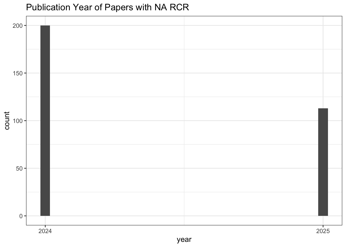
| Version | Author | Date |
|---|---|---|
| 88e1648 | IJbeasley | 2025-08-05 |
# Count of NA RCR publications
all_results |>
  filter(is.na(relative_citation_ratio)) |>
  nrow()
[1] 313# Values for other citation metrics for papers with
# NA RCR
all_results |>
filter(is.na(relative_citation_ratio)) |>
select(field_citation_rate,
expected_citations_per_year,
citation_count,
citations_per_year,
relative_citation_ratio) |>
head() field_citation_rate expected_citations_per_year citation_count
1 13.822219 NA 3
2 10.571710 NA 1
3 NA NA 0
4 14.848473 NA 2
5 8.535105 NA 1
6 5.326717 NA 4
citations_per_year relative_citation_ratio
1 3 NA
2 1 NA
3 0 NA
4 2 NA
5 1 NA
6 4 NA# Publication Year of Paper with zero RCR
all_results |>
filter(relative_citation_ratio == 0) |>
ggplot(aes(x = year)) +
geom_histogram() +
scale_x_continuous(breaks = seq(min(all_results$year, na.rm = TRUE),
max(all_results$year, na.rm = TRUE), 1)) +
theme_bw() +
labs(title = "Publication Year of Papers with Zero RCR")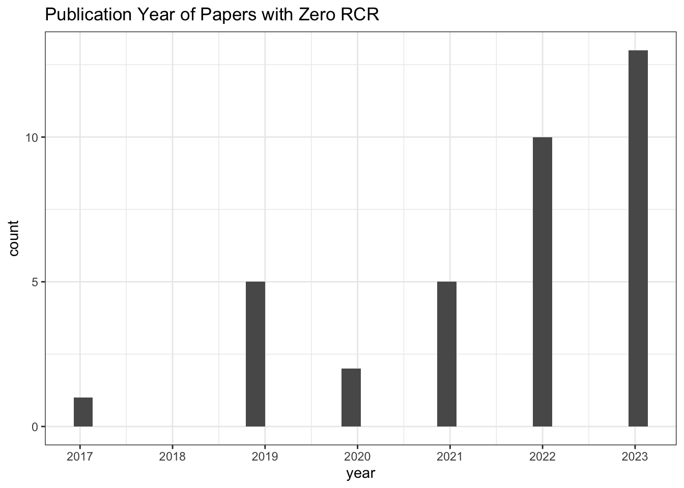
| Version | Author | Date |
|---|---|---|
| 88e1648 | IJbeasley | 2025-08-05 |
# Count of zero RCR publications
all_results |>
  filter(relative_citation_ratio == 0) |>
  nrow()
[1] 36# Values for other citation metrics for papers with
# zero RCR
all_results |>
filter(relative_citation_ratio == 0) |>
select(field_citation_rate,
expected_citations_per_year,
citation_count,
citations_per_year,
relative_citation_ratio) |>
head() field_citation_rate expected_citations_per_year citation_count
1 0.9545455 0.7909298 0
2 3.0000000 1.6893112 0
3 2.1426202 0.8013203 0
4 2.2334348 0.8352841 0
5 2.5710387 0.9615448 0
6 1.2419355 0.4644725 0
citations_per_year relative_citation_ratio
1 0 0
2 0 0
3 0 0
4 0 0
5 0 0
6 0 06. Correlations Between Citation Metrics
# Spearman correlation: citation count vs RCR
cor(all_results$citation_count,
    all_results$relative_citation_ratio,
    method = "spearman",
    use = "pairwise.complete.obs")
[1] 0.8763393# Spearman correlation: citations per year vs RCR
cor(all_results$citations_per_year,
all_results$relative_citation_ratio,
method = "spearman",
use = "pairwise.complete.obs")[1] 0.98679087. Relationships between citation metrics (scatterplots)
# RCR vs citation count (log x-axis)
ggplot(all_results, aes(x = citation_count + 1, y = relative_citation_ratio)) +
  scale_x_log10() +
  geom_point() +
  theme_bw()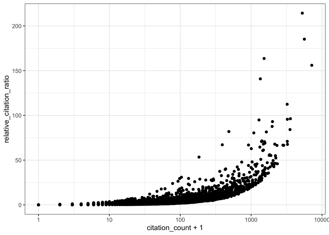
| Version | Author | Date |
|---|---|---|
| 88e1648 | IJbeasley | 2025-08-05 |
# RCR vs expected citations per year
ggplot(all_results, aes(x = expected_citations_per_year, y = relative_citation_ratio)) +
  scale_x_log10() +
  geom_point() +
  theme_bw()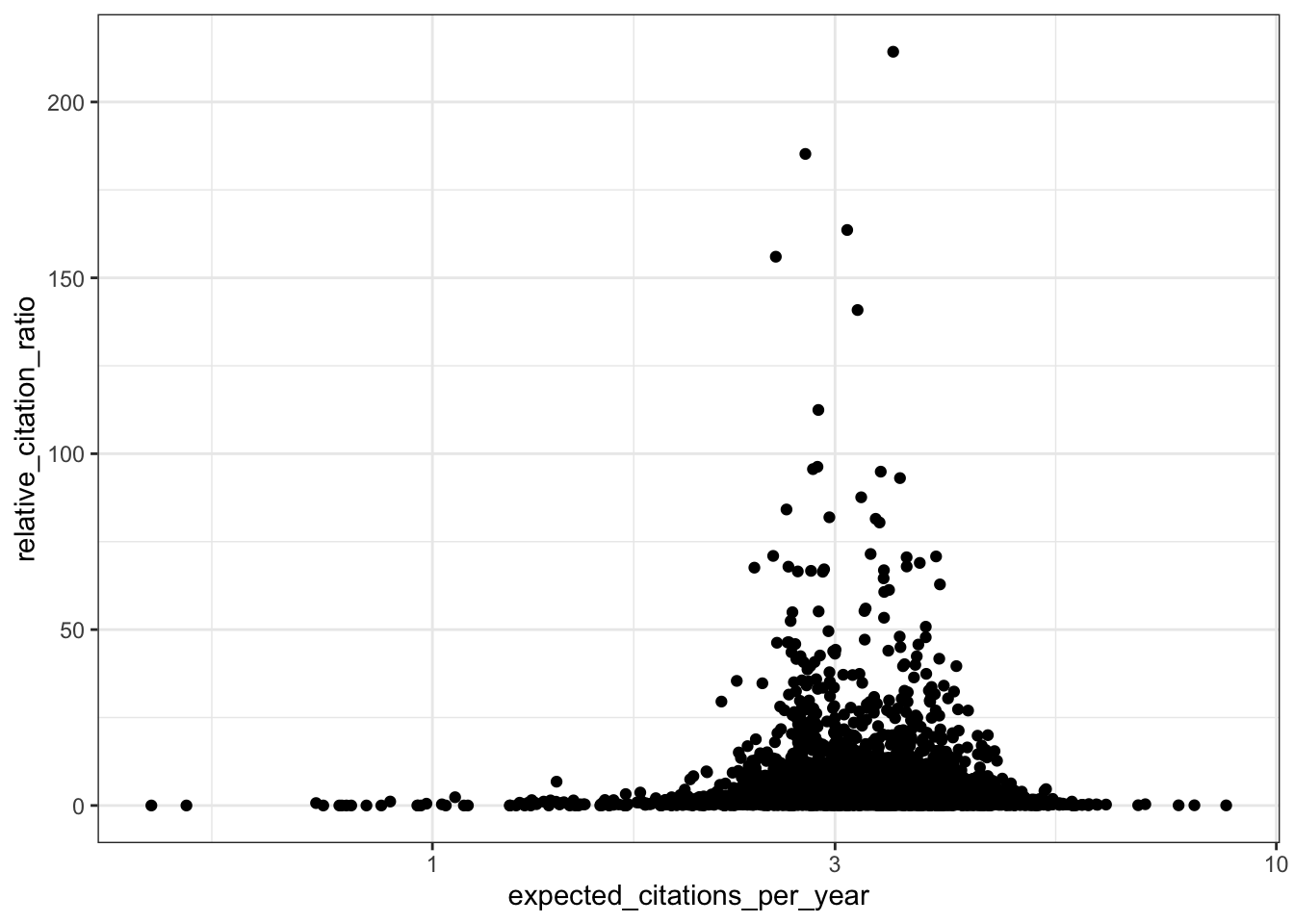
| Version | Author | Date |
|---|---|---|
| 88e1648 | IJbeasley | 2025-08-05 |
# RCR vs field citation rate
ggplot(all_results, aes(x = field_citation_rate, y = relative_citation_ratio)) +
  scale_x_log10() +
  geom_point() +
  theme_bw()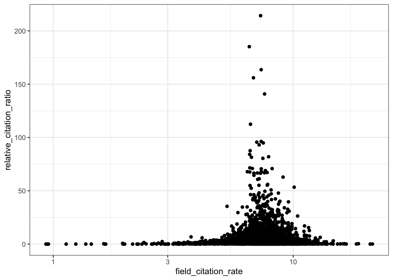
| Version | Author | Date |
|---|---|---|
| 88e1648 | IJbeasley | 2025-08-05 |
8. RCR Over Time (Like in Reales & Wallace)
Reales & Wallace observe bump in the RCR of papers published in the last two years (their conclusion is that citation metrics stabilise after two year) - do we observe the same trend?
# RCR vs publication year (raw scale)
all_results |>
  filter(!is.na(relative_citation_ratio), relative_citation_ratio != 0) |>
  ggplot(aes(x = year, y = relative_citation_ratio)) +
  geom_point() +
  theme_bw() +
  labs(x = 'Year')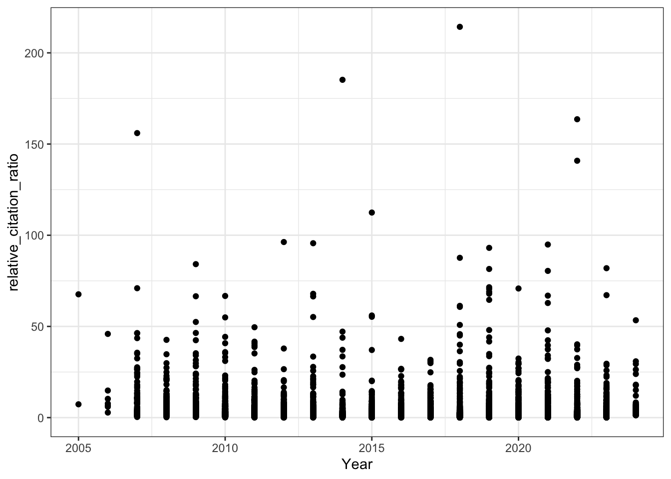
| Version | Author | Date |
|---|---|---|
| 88e1648 | IJbeasley | 2025-08-05 |
# RCR vs year (log y-axis)
all_results |>
  filter(!is.na(relative_citation_ratio), relative_citation_ratio != 0) |>
  ggplot(aes(x = year, y = relative_citation_ratio)) +
  scale_y_log10() +
  geom_point() +
  theme_bw() +
  labs(title = "RCR over time",
       x = 'Year')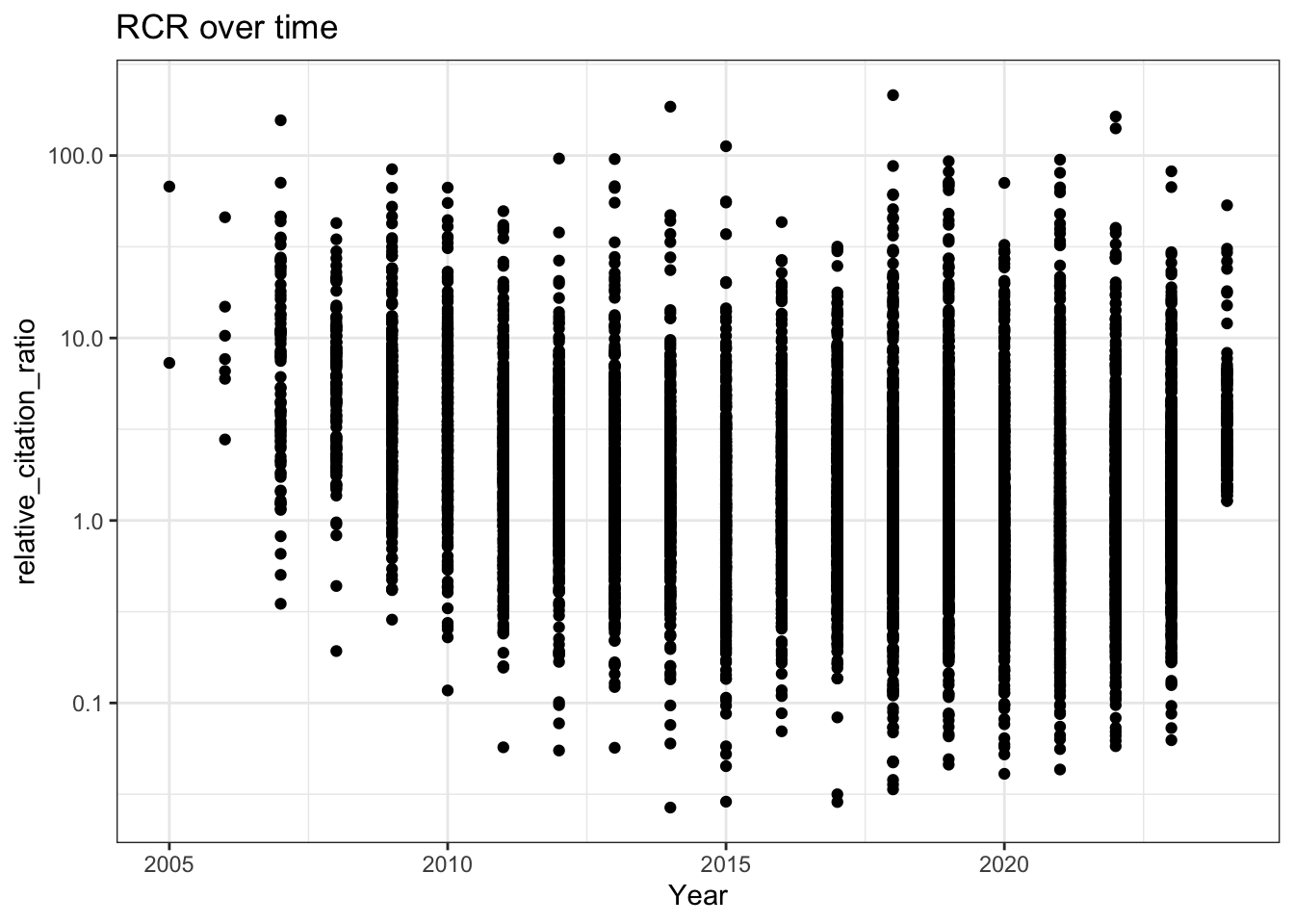
| Version | Author | Date |
|---|---|---|
| 88e1648 | IJbeasley | 2025-08-05 |
# Boxplot of RCRs per year
all_results |>
  filter(!is.na(relative_citation_ratio), relative_citation_ratio != 0) |>
  ggplot(aes(x = factor(year), y = relative_citation_ratio)) +
  geom_boxplot(outlier.size = 0.5) +
  scale_y_log10() +
  theme_bw() +
  labs(x = 'Year')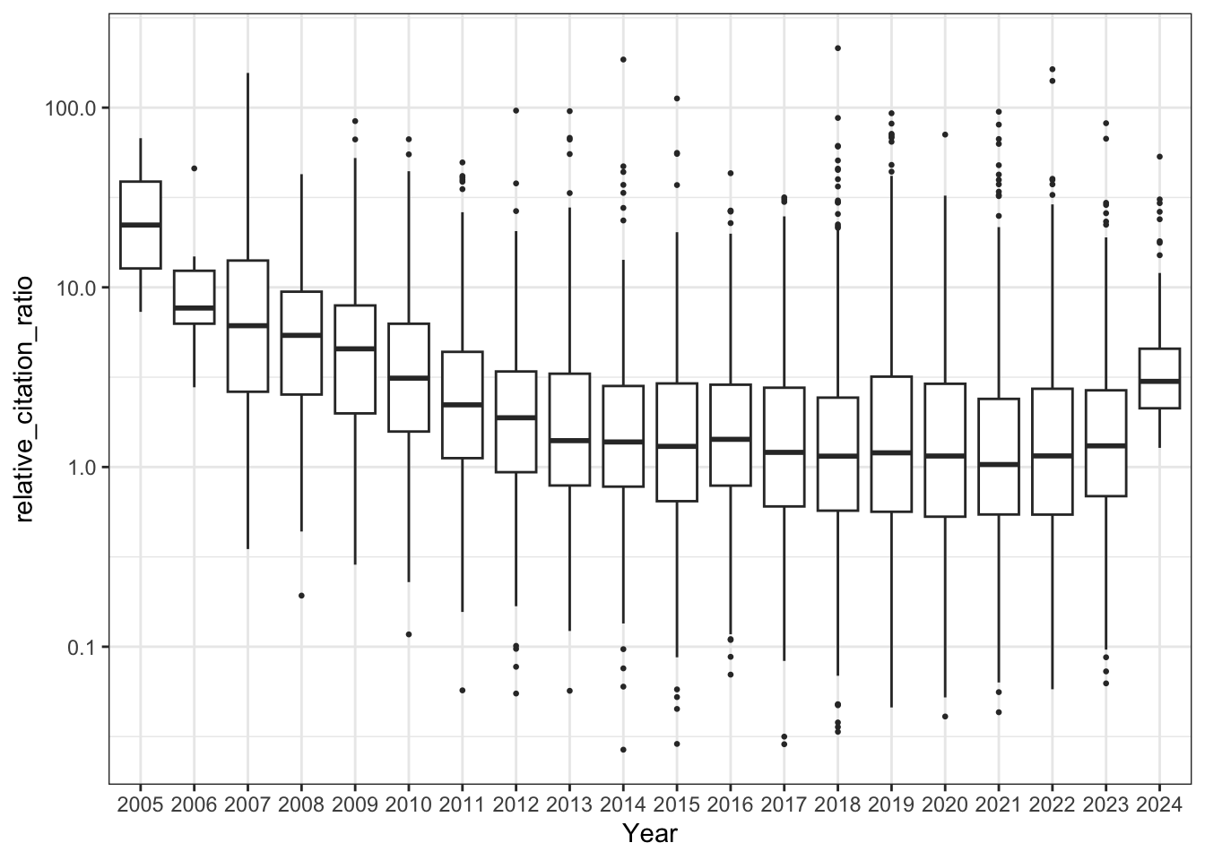
| Version | Author | Date |
|---|---|---|
| 88e1648 | IJbeasley | 2025-08-05 |
# Citations per year over time
all_results |>
  filter(!is.na(relative_citation_ratio), relative_citation_ratio != 0) |>
  ggplot(aes(x = year, y = citations_per_year)) +
  geom_point() +
  theme_bw()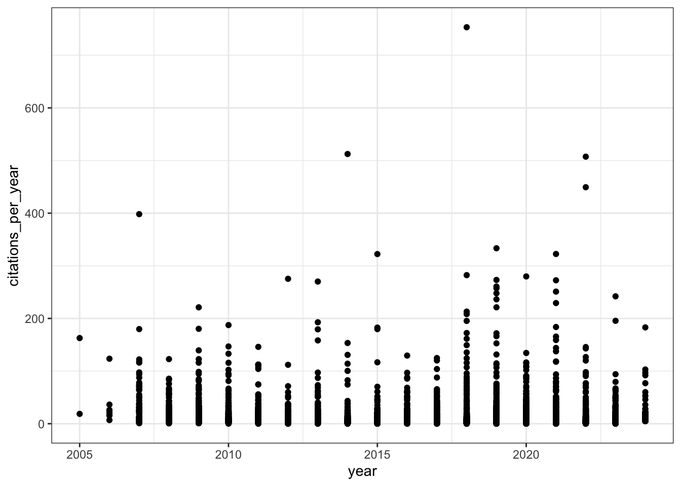
| Version | Author | Date |
|---|---|---|
| 88e1648 | IJbeasley | 2025-08-05 |
sessionInfo()R version 4.3.1 (2023-06-16)
Platform: aarch64-apple-darwin20 (64-bit)
Running under: macOS 15.6
Matrix products: default
BLAS: /Library/Frameworks/R.framework/Versions/4.3-arm64/Resources/lib/libRblas.0.dylib
LAPACK: /Library/Frameworks/R.framework/Versions/4.3-arm64/Resources/lib/libRlapack.dylib; LAPACK version 3.11.0
locale:
[1] en_US.UTF-8/en_US.UTF-8/en_US.UTF-8/C/en_US.UTF-8/en_US.UTF-8
time zone: America/Los_Angeles
tzcode source: internal
attached base packages:
[1] stats graphics grDevices datasets utils methods base
other attached packages:
[1] ggplot2_3.5.2 purrr_1.1.0 data.table_1.17.8 dplyr_1.1.4
[5] jsonlite_2.0.0 httr_1.4.7 workflowr_1.7.1
loaded via a namespace (and not attached):
[1] gtable_0.3.6 compiler_4.3.1 renv_1.0.3 promises_1.3.3
[5] tidyselect_1.2.1 Rcpp_1.1.0 stringr_1.5.1 git2r_0.36.2
[9] callr_3.7.6 later_1.4.2 jquerylib_0.1.4 scales_1.4.0
[13] yaml_2.3.10 fastmap_1.2.0 R6_2.6.1 labeling_0.4.3
[17] generics_0.1.4 curl_6.4.0 knitr_1.50 tibble_3.3.0
[21] rprojroot_2.1.0 RColorBrewer_1.1-3 bslib_0.9.0 pillar_1.11.0
[25] rlang_1.1.6 cachem_1.1.0 stringi_1.8.7 httpuv_1.6.16
[29] xfun_0.52 getPass_0.2-4 fs_1.6.6 sass_0.4.10
[33] cli_3.6.5 withr_3.0.2 magrittr_2.0.3 ps_1.9.1
[37] grid_4.3.1 digest_0.6.37 processx_3.8.6 rstudioapi_0.17.1
[41] lifecycle_1.0.4 vctrs_0.6.5 evaluate_1.0.4 glue_1.8.0
[45] farver_2.1.2 whisker_0.4.1 rmarkdown_2.29 tools_4.3.1
[49] pkgconfig_2.0.3 htmltools_0.5.8.1