Global burden of disease statistics
Isobel Beasley
2025-09-11
Last updated: 2025-09-11
Checks: 7 0
Knit directory:
genomics_ancest_disease_dispar/
This reproducible R Markdown analysis was created with workflowr (version 1.7.1). The Checks tab describes the reproducibility checks that were applied when the results were created. The Past versions tab lists the development history.
Great! Since the R Markdown file has been committed to the Git repository, you know the exact version of the code that produced these results.
Great job! The global environment was empty. Objects defined in the global environment can affect the analysis in your R Markdown file in unknown ways. For reproduciblity it’s best to always run the code in an empty environment.
The command set.seed(20220216) was run prior to running
the code in the R Markdown file. Setting a seed ensures that any results
that rely on randomness, e.g. subsampling or permutations, are
reproducible.
Great job! Recording the operating system, R version, and package versions is critical for reproducibility.
Nice! There were no cached chunks for this analysis, so you can be confident that you successfully produced the results during this run.
Great job! Using relative paths to the files within your workflowr project makes it easier to run your code on other machines.
Great! You are using Git for version control. Tracking code development and connecting the code version to the results is critical for reproducibility.
The results in this page were generated with repository version e692d81. See the Past versions tab to see a history of the changes made to the R Markdown and HTML files.
Note that you need to be careful to ensure that all relevant files for
the analysis have been committed to Git prior to generating the results
(you can use wflow_publish or
wflow_git_commit). workflowr only checks the R Markdown
file, but you know if there are other scripts or data files that it
depends on. Below is the status of the Git repository when the results
were generated:
Ignored files:
    Ignored:    .DS_Store
    Ignored:    .Rproj.user/
    Ignored:    analysis/figure/
    Ignored:    data/.DS_Store
    Ignored:    data/gwas_catalog/
    Ignored:    output/gwas_cat/
    Ignored:    output/gwas_study_info_cohort_corrected.csv
    Ignored:    output/gwas_study_info_trait_corrected.csv
    Ignored:    output/gwas_study_info_trait_ontology_info.csv
    Ignored:    output/gwas_study_info_trait_ontology_info_l1.csv
    Ignored:    output/gwas_study_info_trait_ontology_info_l2.csv
    Ignored:    output/trait_ontology/
    Ignored:    renv/

Untracked files:
    Untracked:  data/gbd/
    Untracked:  data/who/

Unstaged changes:
    Modified:   analysis/index.Rmd
    Deleted:    analysis/level_1_disease_group.Rmd
    Deleted:    analysis/non_ontology_trait_collapse.Rmd
    Deleted:    analysis/trait_ontology_collapse.Rmd
Note that any generated files, e.g. HTML, png, CSS, etc., are not included in this status report because it is ok for generated content to have uncommitted changes.
These are the previous versions of the repository in which changes were
made to the R Markdown (analysis/gbd_data_plots.Rmd) and
HTML (docs/gbd_data_plots.html) files. If you’ve configured
a remote Git repository (see ?wflow_git_remote), click on
the hyperlinks in the table below to view the files as they were in that
past version.
| File | Version | Author | Date | Message |
|---|---|---|---|---|
| Rmd | e692d81 | IJbeasley | 2025-09-11 | Initial investigation into gbd paf |
library(data.table)
library(dplyr)
Attaching package: 'dplyr'The following objects are masked from 'package:data.table':
between, first, lastThe following objects are masked from 'package:stats':
filter, lagThe following objects are masked from 'package:base':
intersect, setdiff, setequal, unionlibrary(ggplot2)
library(stringr)gbd_data <- data.table::fread(here::here("data/gbd/IHME-GBD_2021_DATA-aa22a7fd-1.csv"))Global disease burden - top 15 non-communicable diseases by DALYs (2019)
gbd_data |>
slice_max(n = 15, order_by = val) |>
ggplot(aes(x = reorder(cause, val), y = val)) +
geom_col(fill = "steelblue") +
geom_errorbar(aes(ymin = lower, ymax = upper), width = 0.3) +
coord_flip() +
labs(
x = "Disease",
y = "DALYs (rate per 100,000)",
title = "Non-communicable diseases with the greatest global disease durden (DALYs - 2019)"
) +
theme_minimal(base_size = 14)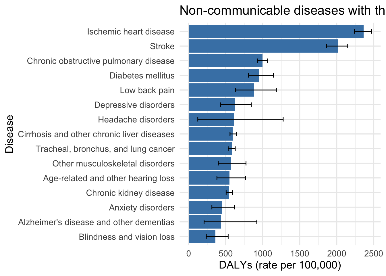 ## Distribution of DALYs (rate per 100,000) for non-communicable
diseases (2019)
## Distribution of DALYs (rate per 100,000) for non-communicable
diseases (2019)
gbd_data |>
  ggplot(aes(x = val)) +
  geom_histogram(bins = 30, fill = "steelblue", color = "black") +
  labs(
    x = "DALYs (rate per 100,000)",
    y = "# non-communicable diseases",
    title = "Distribution of DALYs (rate per 100,000) for non-communicable diseases (2019)"
  ) +
  theme_minimal(base_size = 14)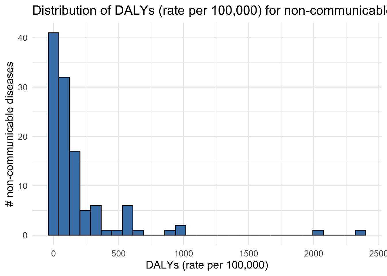
top_non_comm_diseases <- gbd_data |>
  slice_max(n = 15, order_by = val)

top_non_comm_diseases_daly = top_non_comm_diseases |> pull(val)
top_non_comm_diseases = top_non_comm_diseases |> pull(cause)
Global disease burden - Population Attributable Fraction (PAF) for top 15 non-communicable diseases by DALYs (2019)
Load + basic processing of GBD PAF data
gbd_paf_dir <- "data/gbd/IHME_GBD_2021_RISK_1990_2021_RESULTS_APPENDIX_TABLES"

paf_file <- paste0(gbd_paf_dir,
                     "/IHME_GBD_2021_RISK_1990_2021_RESULTS_APPENDIX_TABLE_S1_GLOBAL_Y2024M05D14.XLSX")

gbd_paf_data <- readxl::read_xlsx(here::here(paf_file),
                                  skip = 1
                                  )

# Clean column names
names(gbd_paf_data) <- names(gbd_paf_data) |>
  stringr::str_replace_all("\\r|\\n", " ") |>   # remove carriage returns/newlines
  stringr::str_squish() |>                     # trim extra spaces
  stringr::str_replace_all(" ", "_") |># replace spaces with underscores
  stringr::str_replace("^([0-9]{4})_(.*)$", "\\2_\\1")

# Clean all character cells
gbd_paf_data <- gbd_paf_data |>
  dplyr::mutate(across(where(is.character),
                ~ .x |> stringr::str_replace_all("\\r|\\n", " ") |> stringr::str_squish()))

head(gbd_paf_data)
# A tibble: 6 × 41
Risk_Name Deaths_PAF_1990 Deaths_PAF_2000 Deaths_PAF_2010 Deaths_PAF_2021
<chr> <chr> <chr> <chr> <chr>
1 All risk fact… 59·6 (57·1 – 6… 59·9 (57·4 – 6… 59·7 (56·8 – 6… 50·2 (46·9 – 5…
2 Environmental… 27·3 (24·3 – 3… 25·6 (22·8 – 2… 24·5 (21·8 – 2… 18·9 (16·3 – 2…
3 Unsafe water,… 6·84 (4·83 – 8… 4·91 (3·30 – 6… 3·64 (2·33 – 4… 1·79 (1·07 – 2…
4 Unsafe water … 4·71 (2·76 – 6… 3·34 (1·86 – 4… 2·46 (1·23 – 3… 1·18 (0·547 – …
5 Diarrhoeal di… 74·2 (43·8 – 9… 73·7 (43·0 – 9… 72·1 (40·7 – 9… 68·8 (36·6 – 8…
6 Unsafe sanita… 4·05 (3·13 – 5… 2·81 (2·15 – 3… 1·99 (1·50 – 2… 0·877 (0·624 –…
# ℹ 36 more variables: `Deaths_(in_thousands)_1990` <chr>,
# `Deaths_(in_thousands)_2000` <chr>, `Deaths_(in_thousands)_2010` <chr>,
# `Deaths_(in_thousands)_2021` <chr>,
# `all-age_Deaths_rate_(per_100,000)_1990` <chr>,
# `all-age_Deaths_rate_(per_100,000)_2000` <chr>,
# `all-age_Deaths_rate_(per_100,000)_2010` <chr>,
# `all-age_Deaths_rate_(per_100,000)_2021` <chr>, …Grouping and filtering of GBD PAF data
# remove risk factor rows
gbd_paf_data = gbd_paf_data |>
  rowwise() |>
  mutate(causal_group = ifelse(grepl("All causes", Risk_Name), Risk_Name, NA)) |>
  ungroup() |>
  tidyr::fill(causal_group, .direction = "down") |>
  relocate(causal_group, .before = Risk_Name)


gbd_paf_data = gbd_paf_data |>
  filter(!grepl("All causes", Risk_Name)) |>
  mutate(causal_group = stringr::str_remove_all(causal_group, ": All causes"))


head(gbd_paf_data)
# A tibble: 6 × 42
causal_group Risk_Name Deaths_PAF_1990 Deaths_PAF_2000 Deaths_PAF_2010
<chr> <chr> <chr> <chr> <chr>
1 Unsafe water source Diarrhoe… 74·2 (43·8 – 9… 73·7 (43·0 – 9… 72·1 (40·7 – 9…
2 Unsafe sanitation Diarrhoe… 63·6 (57·9 – 6… 62·1 (56·4 – 6… 58·5 (52·6 – 6…
3 No access to handwa… Diarrhoe… 23·6 (3·36 – 4… 23·8 (3·38 – 4… 22·7 (3·23 – 4…
4 No access to handwa… Lower re… 14·7 (-10·7 – … 14·0 (-10·3 – … 12·6 (-9·07 – …
5 Ambient particulate… Diarrhoe… 0·256 (0·157 –… 0·216 (0·135 –… 0·176 (0·105 –…
6 Ambient particulate… Lower re… 9·26 (1·83 – 1… 10·0 (2·02 – 1… 10·9 (2·02 – 1…
# ℹ 37 more variables: Deaths_PAF_2021 <chr>,
# `Deaths_(in_thousands)_1990` <chr>, `Deaths_(in_thousands)_2000` <chr>,
# `Deaths_(in_thousands)_2010` <chr>, `Deaths_(in_thousands)_2021` <chr>,
# `all-age_Deaths_rate_(per_100,000)_1990` <chr>,
# `all-age_Deaths_rate_(per_100,000)_2000` <chr>,
# `all-age_Deaths_rate_(per_100,000)_2010` <chr>,
# `all-age_Deaths_rate_(per_100,000)_2021` <chr>, …gbd_paf_data |>
select(causal_group, Risk_Name, DALYs_PAF_2021, 'all-age_DALYs_rate_(per_100,000)_2021') |>
distinct() |>
arrange(Risk_Name)# A tibble: 707 × 4
causal_group Risk_Name DALYs_PAF_2021 all-age_DALYs_rate_(…¹
<chr> <chr> <chr> <chr>
1 Drug use Acute he… 1·04 (0·630 –… 0·3 (0·1 – 0·4)
2 Drug use Acute he… 28·1 (19·3 – … 0·9 (0·4 – 1·7)
3 Occupational exposure to ben… Acute ly… 0·728 (0·212 … 0·3 (0·1 – 0·6)
4 Occupational exposure to for… Acute ly… 0·274 (0·222 … 0·1 (0·1 – 0·2)
5 Smoking Acute ly… 2·70 (0·988 –… 1·3 (0·4 – 2·2)
6 High body-mass index Acute ly… 4·02 (2·99 – … 1·9 (1·2 – 2·5)
7 Occupational exposure to ben… Acute my… 0·829 (0·243 … 0·4 (0·1 – 0·7)
8 Occupational exposure to for… Acute my… 0·264 (0·223 … 0·1 (0·1 – 0·2)
9 Smoking Acute my… 7·47 (2·76 – … 3·9 (1·4 – 6·7)
10 High body-mass index Acute my… 7·76 (5·79 – … 4·1 (3·0 – 5·3)
# ℹ 697 more rows
# ℹ abbreviated name: ¹`all-age_DALYs_rate_(per_100,000)_2021`Looking into 2021 PAF data for top 15 non-communicable diseases by DALYs (2019)
gbd_paf_data <- gbd_paf_data |>
  # Work just on the DALYs_PAF_2021 column
  mutate(DALYs_PAF_2021 = str_replace_all(DALYs_PAF_2021, "·", ".")) |>  # replace middle dot with .
  tidyr::extract(
    DALYs_PAF_2021,
    into = c("val", "lower", "upper"),
    regex = "([0-9.]+) \\(([-0-9.]+) – ([-0-9.]+)\\)",
    convert = TRUE
  )


gbd_paf_data |>
  select(val, lower, upper, Risk_Name)|>
  filter(Risk_Name == "Chronic kidney disease")
# A tibble: 0 × 4
# ℹ 4 variables: val <dbl>, lower <dbl>, upper <dbl>, Risk_Name <chr>gbd_paf_plot_data =
gbd_paf_data |>
select(val, lower, upper, Risk_Name) |>
filter(grepl(paste0(top_non_comm_diseases, collapse = "|"), Risk_Name)) |>
mutate(Risk_Name =
case_when(grepl("Chronic kidney disease due to", Risk_Name) ~ "Chronic kidney disease",
TRUE ~ Risk_Name
)) |>
group_by(Risk_Name) |>
summarise(val = sum(val, na.rm = TRUE),
lower = sum(lower, na.rm = TRUE),
upper = sum(upper, na.rm = TRUE)
)
left_join(gbd_paf_plot_data,
data.frame(Risk_Name = top_non_comm_diseases,
daly = top_non_comm_diseases),
by = "Risk_Name") |>
mutate(Risk_Name = factor(Risk_Name, levels = unique(Risk_Name))) |>
ggplot(aes(x = reorder(Risk_Name, val), y = val)) +
geom_col(fill = "steelblue") +
geom_errorbar(aes(ymin = lower, ymax = upper), width = 0.3) +
coord_flip() +
labs(
x = "Risk factor",
y = "Population Attributable Fraction (%)",
title = "Risk factors with the greatest global disease burden (PAF - 2021)"
) +
theme_minimal(base_size = 14)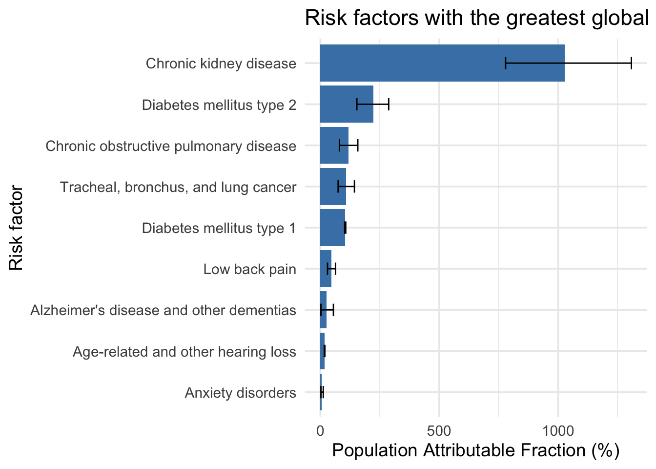
sessionInfo()R version 4.3.1 (2023-06-16)
Platform: aarch64-apple-darwin20 (64-bit)
Running under: macOS 15.6.1
Matrix products: default
BLAS: /Library/Frameworks/R.framework/Versions/4.3-arm64/Resources/lib/libRblas.0.dylib
LAPACK: /Library/Frameworks/R.framework/Versions/4.3-arm64/Resources/lib/libRlapack.dylib; LAPACK version 3.11.0
locale:
[1] en_US.UTF-8/en_US.UTF-8/en_US.UTF-8/C/en_US.UTF-8/en_US.UTF-8
time zone: America/Los_Angeles
tzcode source: internal
attached base packages:
[1] stats graphics grDevices datasets utils methods base
other attached packages:
[1] stringr_1.5.1 ggplot2_3.5.2 dplyr_1.1.4 data.table_1.17.8
[5] workflowr_1.7.1
loaded via a namespace (and not attached):
[1] sass_0.4.10 utf8_1.2.6 generics_0.1.4 tidyr_1.3.1
[5] renv_1.0.3 stringi_1.8.7 digest_0.6.37 magrittr_2.0.3
[9] evaluate_1.0.4 grid_4.3.1 RColorBrewer_1.1-3 fastmap_1.2.0
[13] cellranger_1.1.0 rprojroot_2.1.0 jsonlite_2.0.0 processx_3.8.6
[17] whisker_0.4.1 ps_1.9.1 promises_1.3.3 httr_1.4.7
[21] purrr_1.1.0 scales_1.4.0 jquerylib_0.1.4 cli_3.6.5
[25] rlang_1.1.6 withr_3.0.2 cachem_1.1.0 yaml_2.3.10
[29] tools_4.3.1 httpuv_1.6.16 here_1.0.1 vctrs_0.6.5
[33] R6_2.6.1 lifecycle_1.0.4 git2r_0.36.2 fs_1.6.6
[37] pkgconfig_2.0.3 callr_3.7.6 pillar_1.11.0 bslib_0.9.0
[41] later_1.4.2 gtable_0.3.6 glue_1.8.0 Rcpp_1.1.0
[45] xfun_0.52 tibble_3.3.0 tidyselect_1.2.1 rstudioapi_0.17.1
[49] knitr_1.50 farver_2.1.2 htmltools_0.5.8.1 rmarkdown_2.29
[53] labeling_0.4.3 compiler_4.3.1 getPass_0.2-4 readxl_1.4.5