alt_mediation

Introduction

An alternative mediation analysis examining the possibility of a species:frequency interaction term effect, as proposed by Reviewer 3.

# This script contains functions for fitting
# a linear model under the limma framework
# where the sample covariate value is differnet for each gene
# in this case, and includes and interaction term of condition and linear covariate
# note that the dimension of the expression matrix
# is the same as the dimension of the covariate matrix

library(limma)

Warning: package 'limma' was built under R version 3.4.3

library(assertthat)

library(data.table)

Warning: package 'data.table' was built under R version 3.4.4

lmFit_varying <- function(object, group_vector = NULL, cov_matrix = NULL,
#                   ndups = 1, spacing = 1, block = NULL, 
                   weights = NULL, method = "ls", ...) 
{
  # match dimension of design matrix and covariate matrix
  # the function will stop executing if their dimensions are not the same
  assertthat::assert_that(are_equal(dim(object),dim(cov_matrix)))

  fit <- lm.series_varying(M=object, cov_matrix=cov_matrix,
                           group_vector = group_vector, 
                           weights = weights)
    
  fit$genes <- rownames(object)
  fit$Amean <- rowMeans(object, na.rm = TRUE)
  fit$method <- method
  fit$design <- design
  new("MArrayLM", fit)
}

#' modified lm.series for interaction analysis
#' 
#' @description main worker inside lmFit for our model of interest
#' 
#' @param object matrix of log-expression
#' @param design a vector of sample labels. use model.matrix to make design matrix.
#' @param cov_matrix matrix of covariate values. should be the same dimension
#'         as object.
#'         
#' @author Joyce Hsiao
lm.series_varying <- function (M, cov_matrix,
    group_vector = NULL, weights = NULL)
{
  
  M <- as.matrix(M)
  narrays <- ncol(M)
  
  # make design matrix (not including covariates)
  design <- model.matrix(~group_vector)
  
  # compute the number of regression coefs. to be estimated
  nbeta <- ncol(design) + 2
  
  # make coeffcient names
  coef.names <- c(colnames(design), "HiC", "interact")
  if (is.null(colnames(design))){
    coef.names <- c(paste("x", 1:ncol(design), sep = ""), "HiC", "interact")
  }

  # for every gene, affirm that the expression weights are
  # finite and non-zero
  if (!is.null(weights)) {
    weights <- asMatrixWeights(weights, dim(M))
    weights[weights <= 0] <- NA
    M[!is.finite(weights)] <- NA
  }
  
  ngenes <- nrow(M)
  stdev.unscaled <- beta <- matrix(NA, ngenes, nbeta, dimnames = list(rownames(M), 
                                                                      coef.names))
  

  # start estimating beta coefficients here
  beta <- stdev.unscaled
  sigma <- rep(NA, ngenes)
  df.residual <- rep(0, ngenes)
  for (i in 1:ngenes) {
#    print(i)
    cc <- as.vector(unlist(cov_matrix[i,]))
    design_gene <- model.matrix(~group_vector+cc+cc*group_vector)
    colnames(design_gene) <- coef.names
    y <- as.vector(M[i, ])
    obs <- is.finite(y)
    if (sum(obs) > 0) {
      X <- design_gene[obs, , drop = FALSE]
      y <- y[obs]
      if (is.null(weights)) 
        out <- lm.fit(X, y)
      else {
        w <- as.vector(weights[i, obs])
        out <- lm.wfit(X, y, w)
      }
      est <- !is.na(out$coef)
      beta[i, ] <- out$coef
      stdev.unscaled[i, est] <- sqrt(diag(chol2inv(out$qr$qr, 
                                                   size = out$rank)))
      df.residual[i] <- out$df.residual
      if (df.residual[i] > 0) 
        sigma[i] <- sqrt(mean(out$effects[-(1:out$rank)]^2))
    }
  }
  QR <- qr(design_gene)
  cov.coef <- chol2inv(QR$qr, size = QR$rank)
  est <- QR$pivot[1:QR$rank]
  dimnames(cov.coef) <- list(coef.names[est], coef.names[est])
  list(coefficients = beta, stdev.unscaled = stdev.unscaled, 
       sigma = sigma, df.residual = df.residual, cov.coefficients = cov.coef, 
       pivot = QR$pivot, rank = QR$rank)
}


df <- fread("~/Desktop/Hi-C/joyce_mediation/HiC.data")

df_hic <- df[,c(1,9:16)]
head(df_hic)

             genes A_21792_HIC B_28126_HIC C_3649_HIC D_40300_HIC
1: ENSG00000160087  1.08688722   0.9308794  0.8452477   0.4076793
2: ENSG00000127054  0.79030376   0.5512300  0.6384713   0.5998139
3: ENSG00000240731  0.79030376   0.5512300  0.6384713   0.5998139
4: ENSG00000224051  0.37733343   0.4628101  0.6796571   0.9807702
5: ENSG00000107404  0.61419647   0.5646673  0.0951685   0.2700779
6: ENSG00000175756 -0.02453671   0.6407394  0.9644112   1.0124547
   E_28815_HIC F_28834_HIC  G_3624_HIC H_3651_HIC
1:   0.9411242  1.09245242  0.49777463 0.58755514
2:   0.5308121  0.67897911  0.65454221 0.49264758
3:   0.5308121  0.67897911  0.65454221 0.49264758
4:   0.2967155  0.20317751  1.02449016 0.62904609
5:   0.7123887  0.92062137 -0.03499986 0.09947955
6:   0.2476291  0.01584516  0.90435656 0.92436061

df_counts <- readRDS("~/Desktop/Hi-C/joyce_mediation/count.data.RDS")
df_counts <- data.frame(df_counts)
df_counts$genes <- rownames(df_counts)

library(tidyverse)

Warning: package 'tidyverse' was built under R version 3.4.2

── Attaching packages ────────────────────────────────── tidyverse 1.2.1 ──

✔ ggplot2 3.1.0       ✔ purrr   0.3.2  
✔ tibble  2.1.1       ✔ dplyr   0.8.0.1
✔ tidyr   0.8.3       ✔ stringr 1.4.0  
✔ readr   1.3.1       ✔ forcats 0.4.0  

Warning: package 'tibble' was built under R version 3.4.4

Warning: package 'tidyr' was built under R version 3.4.4

Warning: package 'readr' was built under R version 3.4.4

Warning: package 'purrr' was built under R version 3.4.4

Warning: package 'dplyr' was built under R version 3.4.4

Warning: package 'stringr' was built under R version 3.4.4

Warning: package 'forcats' was built under R version 3.4.4

── Conflicts ───────────────────────────────────── tidyverse_conflicts() ──
✖ dplyr::between()   masks data.table::between()
✖ dplyr::filter()    masks stats::filter()
✖ dplyr::first()     masks data.table::first()
✖ tibble::has_name() masks assertthat::has_name()
✖ dplyr::lag()       masks stats::lag()
✖ dplyr::last()      masks data.table::last()
✖ purrr::transpose() masks data.table::transpose()

# merge count data with the HiC dataframe
df_combo <- left_join(df_hic, df_counts)

Joining, by = "genes"

# Hi-C
cov_matrix <- df_combo[,2:9]
counts <- df_combo[,10:17]
rownames(counts) <- df_combo$genes
rownames(cov_matrix) <- df_combo$genes
species <- factor(c(1,1,2,2,1,1,2,2))
design <- model.matrix(~species)

# compute weights
v <- voom(counts,design=model.matrix(~species), plot=T)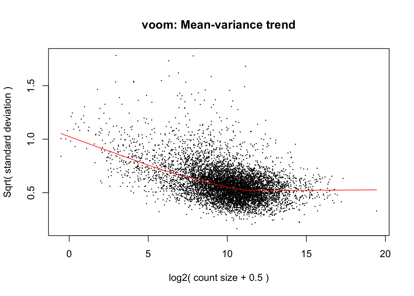

weights <- v$weights
log2cpm <- v$E

fit <- lmFit_varying(object=log2cpm, group_vector=species, cov_matrix=cov_matrix,
                     weights=weights)

fit <- eBayes(fit, robust=TRUE)
myintergenes <- topTable(fit, coef=4, number=Inf)
sum(myintergenes$adj.P.Val<=0.05) #With multiple testing correction, none are significant.

[1] 0

sum(myintergenes$P.Value<=0.05)

[1] 395

#sum(mygenes %in% filter(myintergenes, adj.P.Val<=0.8)$ID)

colors <- c(rep("black", 2), rep("red", 2), rep("black", 2), rep("red", 2))
plot(log2cpm[rownames(log2cpm)=="ENSG00000170561",], cov_matrix[rownames(log2cpm)=="ENSG00000170561",], col=colors)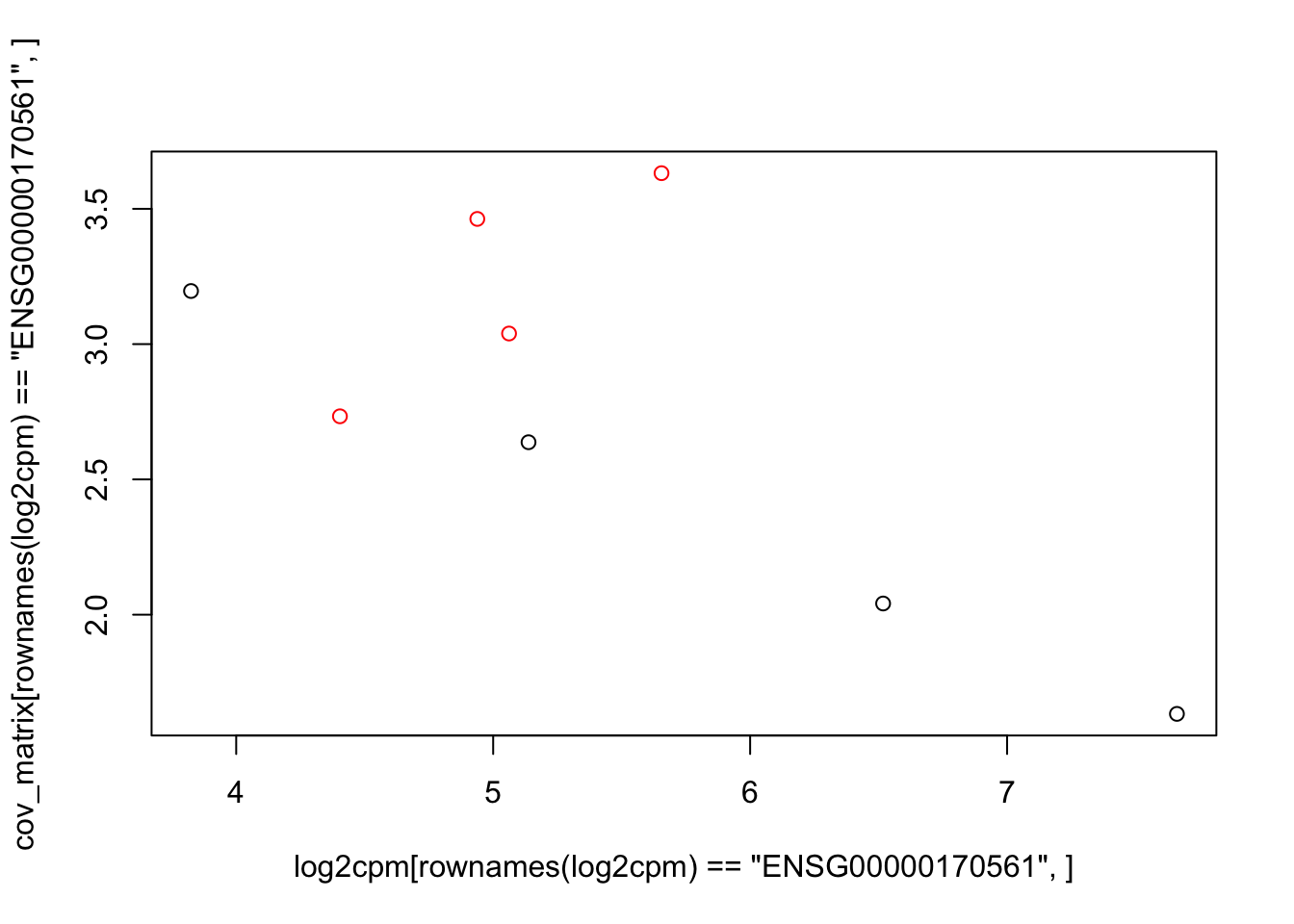

plot(log2cpm[rownames(log2cpm)=="ENSG00000280143",], cov_matrix[rownames(log2cpm)=="ENSG00000280143",], col=colors)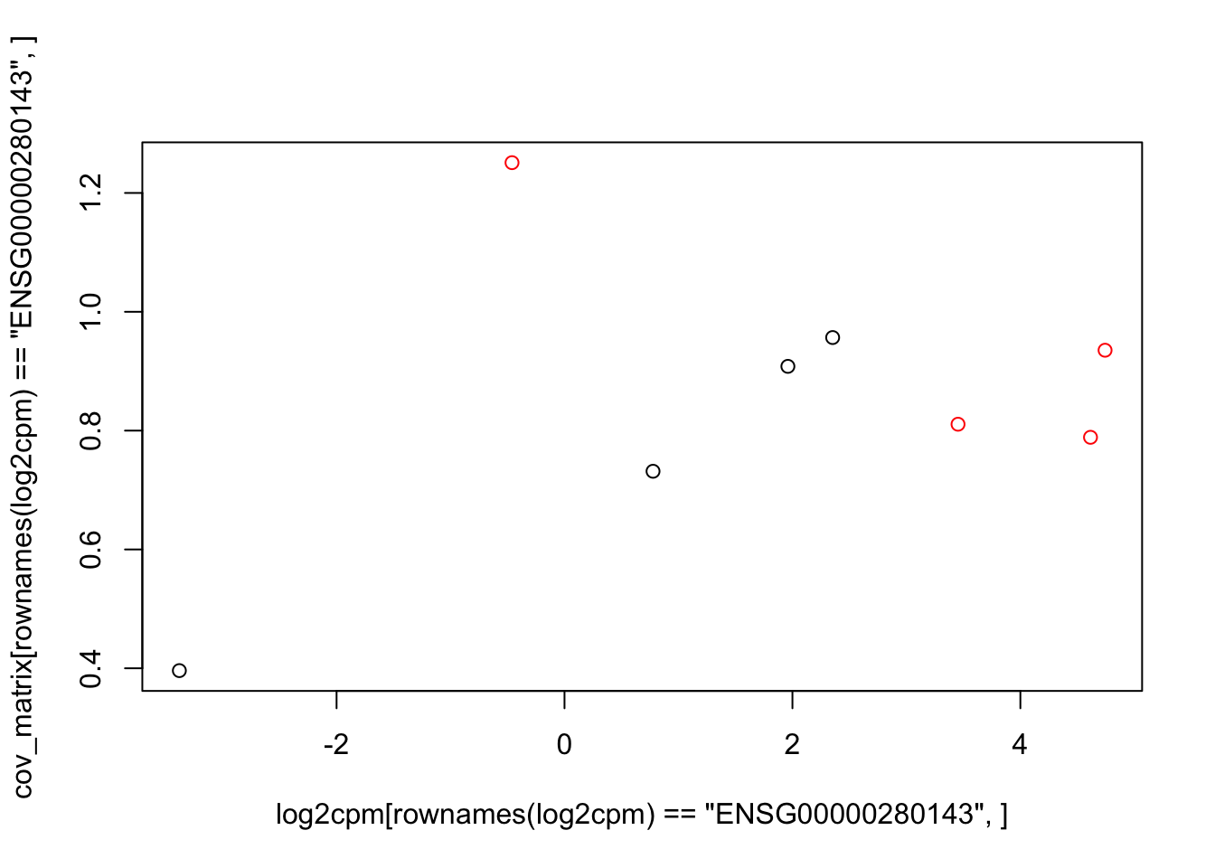

plot(log2cpm[rownames(log2cpm)=="ENSG00000124486",], cov_matrix[rownames(log2cpm)=="ENSG00000124486",], col=colors)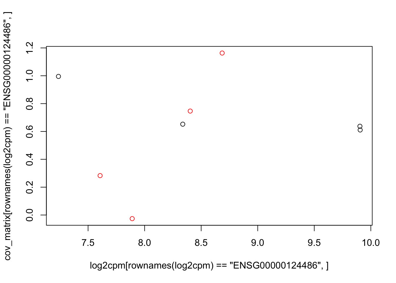

plot(log2cpm[rownames(log2cpm)=="ENSG00000100167",], cov_matrix[rownames(log2cpm)=="ENSG00000100167",], col=colors)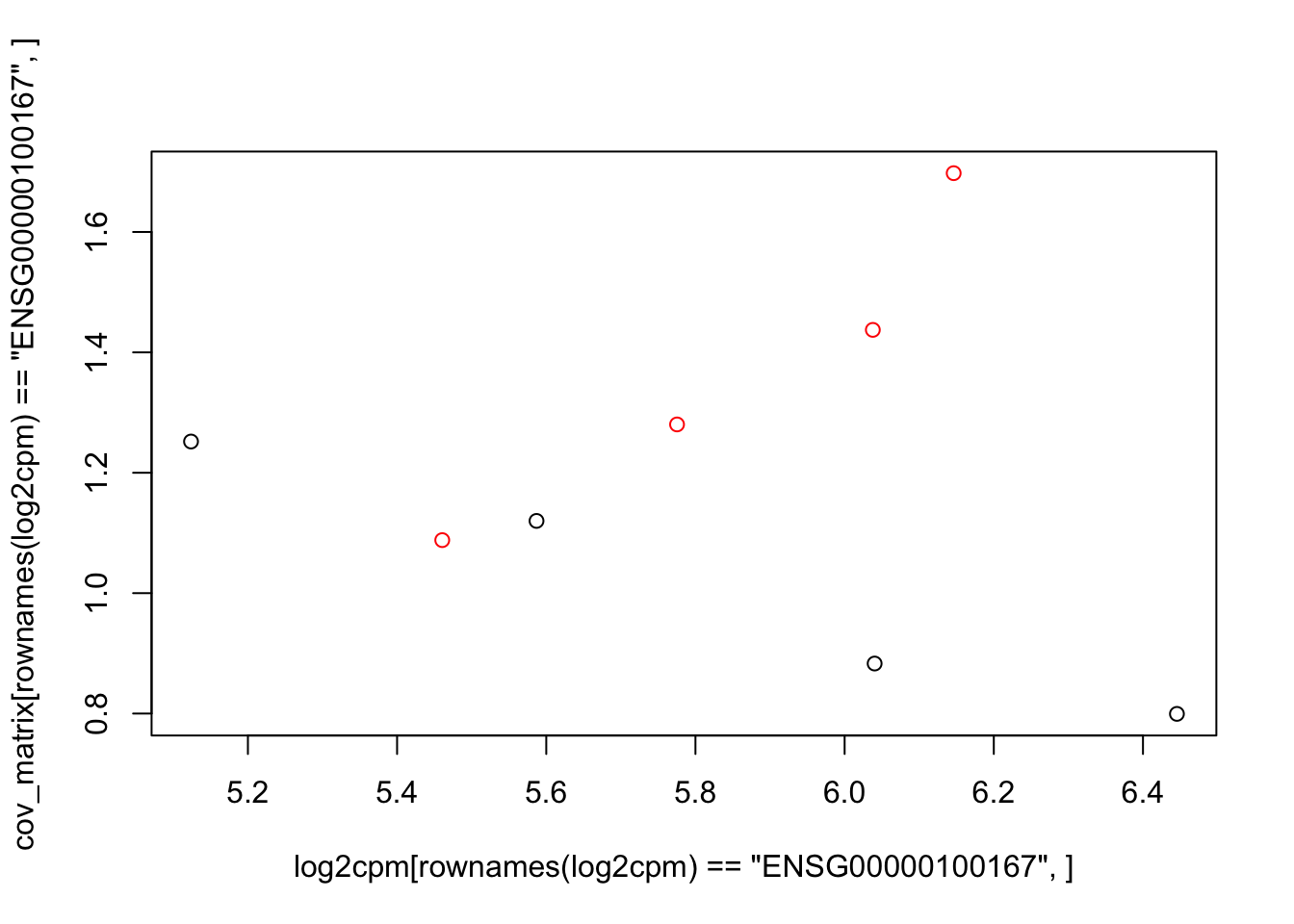

plot(log2cpm[rownames(log2cpm)=="ENSG00000188070",], cov_matrix[rownames(log2cpm)=="ENSG00000188070",], col=colors)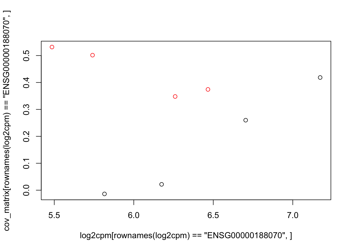

plot(log2cpm[rownames(log2cpm)=="ENSG00000169442",], cov_matrix[rownames(log2cpm)=="ENSG00000169442",], col=colors)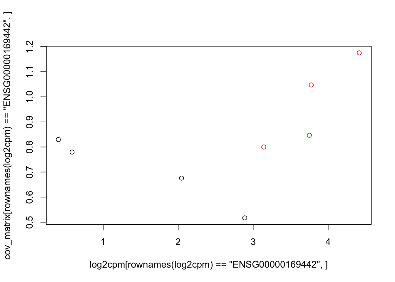

plot(log2cpm[rownames(log2cpm)=="ENSG00000170775",], cov_matrix[rownames(log2cpm)=="ENSG00000170775",], col=colors)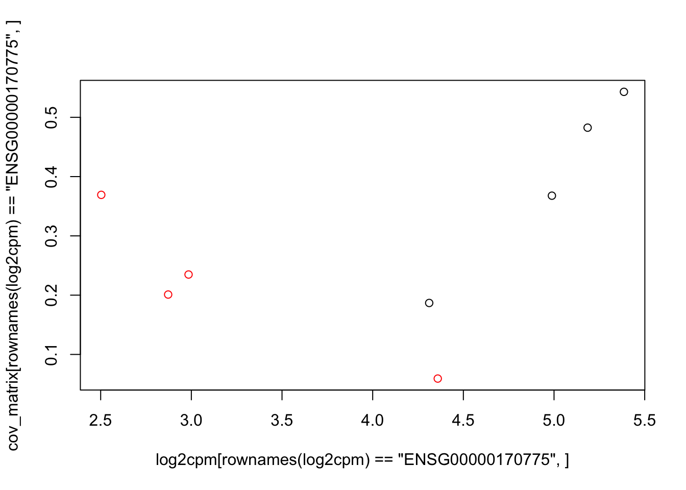

plot(log2cpm[rownames(log2cpm)=="ENSG00000267886",], cov_matrix[rownames(log2cpm)=="ENSG00000267886",], col=colors)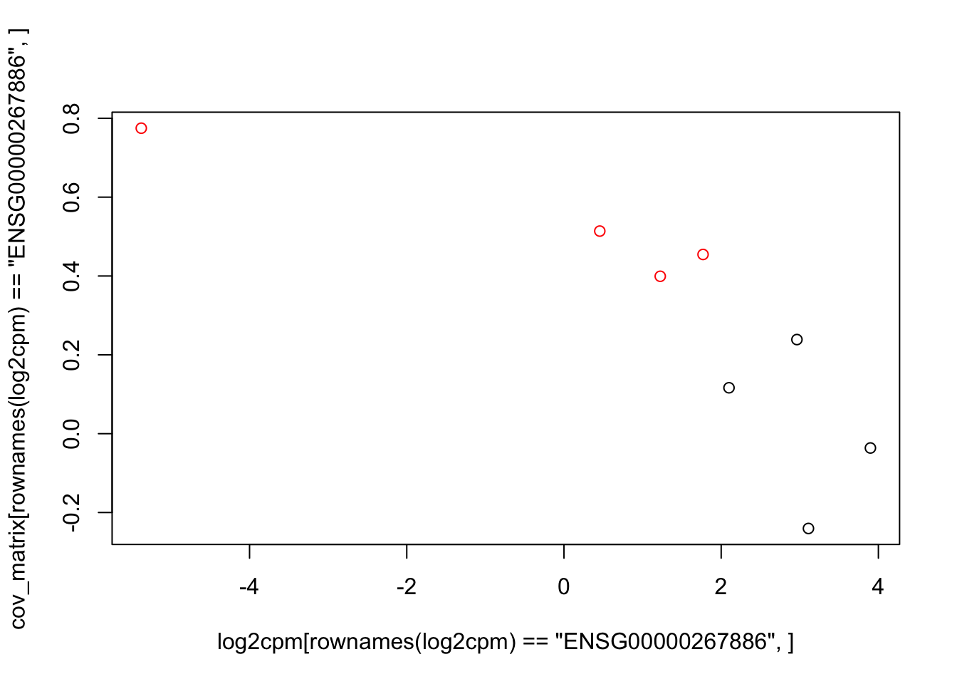

plot(log2cpm[rownames(log2cpm)=="ENSG00000228709",], cov_matrix[rownames(log2cpm)=="ENSG00000228709",], col=colors)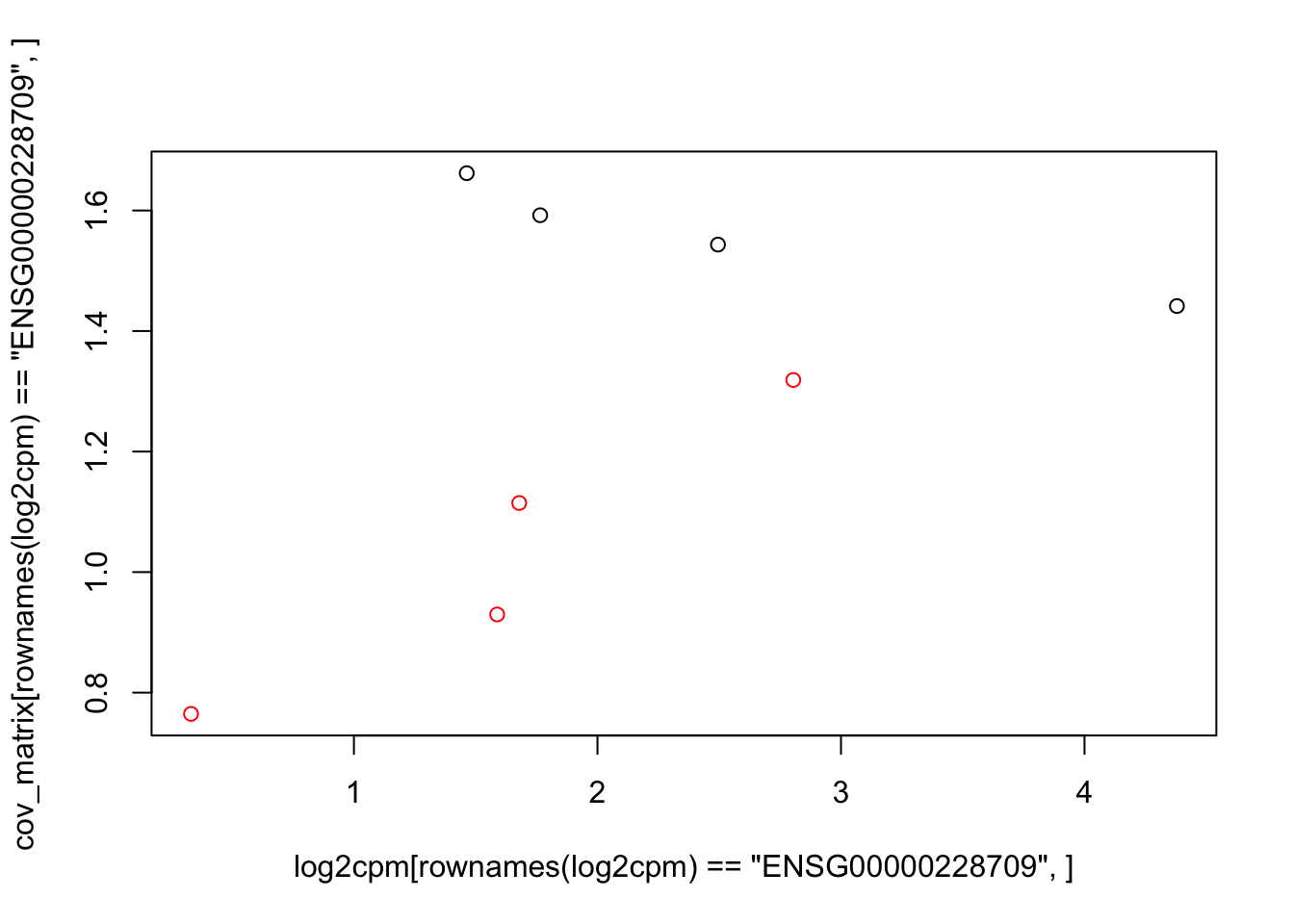

plot(log2cpm[rownames(log2cpm)=="ENSG00000178718",], cov_matrix[rownames(log2cpm)=="ENSG00000178718",], col=colors)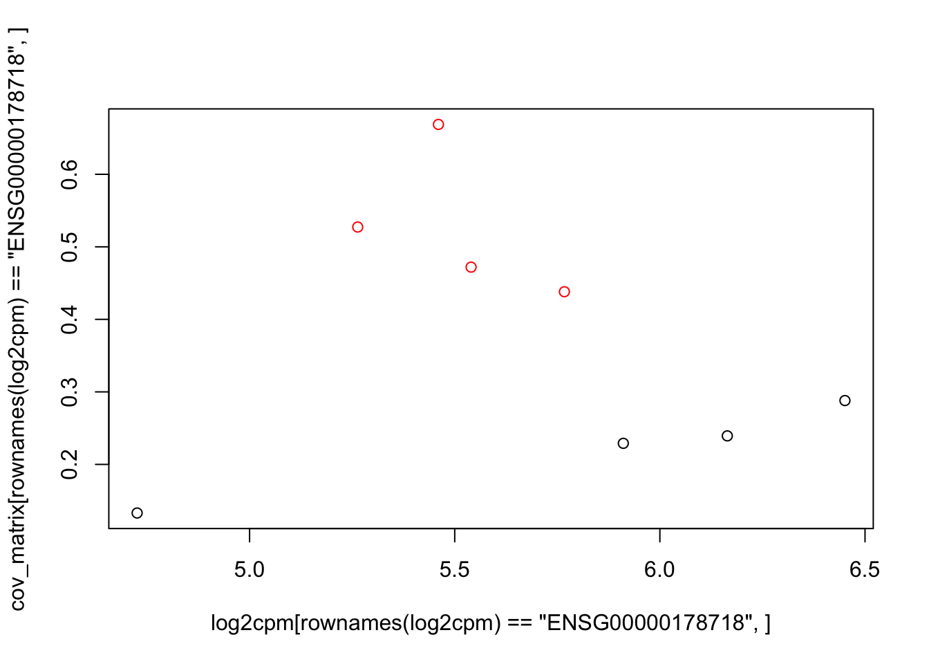

plot(log2cpm[rownames(log2cpm)=="ENSG00000133636",], cov_matrix[rownames(log2cpm)=="ENSG00000133636",], col=colors)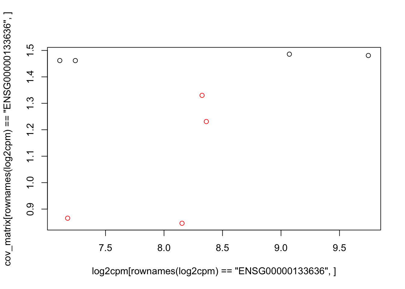

plot(log2cpm[rownames(log2cpm)=="ENSG00000204252",], cov_matrix[rownames(log2cpm)=="ENSG00000204252",], col=colors)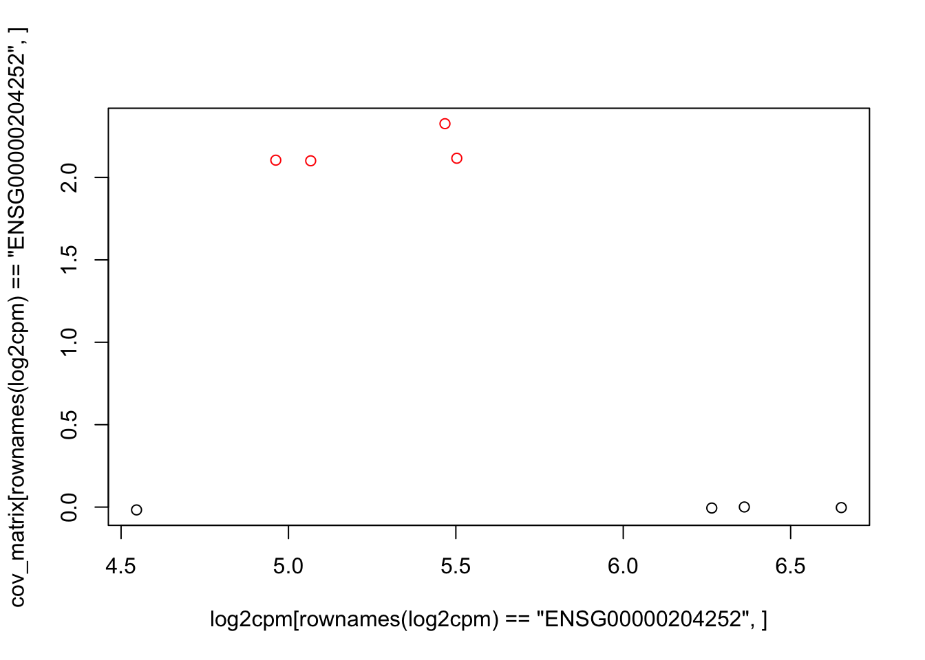

Session information

sessionInfo()

R version 3.4.0 (2017-04-21)
Platform: x86_64-apple-darwin15.6.0 (64-bit)
Running under: OS X El Capitan 10.11.6

Matrix products: default
BLAS: /Library/Frameworks/R.framework/Versions/3.4/Resources/lib/libRblas.0.dylib
LAPACK: /Library/Frameworks/R.framework/Versions/3.4/Resources/lib/libRlapack.dylib

locale:
[1] en_US.UTF-8/en_US.UTF-8/en_US.UTF-8/C/en_US.UTF-8/en_US.UTF-8

attached base packages:
[1] stats     graphics  grDevices utils     datasets  methods   base     

other attached packages:
 [1] forcats_0.4.0     stringr_1.4.0     dplyr_0.8.0.1    
 [4] purrr_0.3.2       readr_1.3.1       tidyr_0.8.3      
 [7] tibble_2.1.1      ggplot2_3.1.0     tidyverse_1.2.1  
[10] data.table_1.12.0 assertthat_0.2.1  limma_3.34.9     

loaded via a namespace (and not attached):
 [1] statmod_1.4.30   tidyselect_0.2.5 xfun_0.5         haven_2.1.0     
 [5] lattice_0.20-38  colorspace_1.4-1 generics_0.0.2   htmltools_0.3.6 
 [9] yaml_2.2.0       rlang_0.3.3      pillar_1.3.1     glue_1.3.1      
[13] withr_2.1.2      modelr_0.1.4     readxl_1.3.1     plyr_1.8.4      
[17] munsell_0.5.0    gtable_0.3.0     workflowr_1.2.0  cellranger_1.1.0
[21] rvest_0.3.2      evaluate_0.13    knitr_1.22       broom_0.5.1     
[25] Rcpp_1.0.1       scales_1.0.0     backports_1.1.3  jsonlite_1.6    
[29] fs_1.2.7         hms_0.4.2        digest_0.6.18    stringi_1.4.3   
[33] grid_3.4.0       rprojroot_1.3-2  cli_1.1.0        tools_3.4.0     
[37] magrittr_1.5     lazyeval_0.2.2   crayon_1.3.4     whisker_0.3-2   
[41] pkgconfig_2.0.2  xml2_1.2.0       lubridate_1.7.4  rmarkdown_1.12  
[45] httr_1.4.0       rstudioapi_0.10  R6_2.4.0         nlme_3.1-137    
[49] git2r_0.25.2     compiler_3.4.0