Overlaying Hi-C with Gene Expression
Ittai Eres
2019-03-14
Last updated: 2019-03-14
Checks: 6 0
Knit directory: HiCiPSC/
This reproducible R Markdown analysis was created with workflowr (version 1.2.0). The Report tab describes the reproducibility checks that were applied when the results were created. The Past versions tab lists the development history.
Great! Since the R Markdown file has been committed to the Git repository, you know the exact version of the code that produced these results.
Great job! The global environment was empty. Objects defined in the global environment can affect the analysis in your R Markdown file in unknown ways. For reproduciblity it’s best to always run the code in an empty environment.
The command set.seed(20190311) was run prior to running the code in the R Markdown file. Setting a seed ensures that any results that rely on randomness, e.g. subsampling or permutations, are reproducible.
Great job! Recording the operating system, R version, and package versions is critical for reproducibility.
Nice! There were no cached chunks for this analysis, so you can be confident that you successfully produced the results during this run.
Great! You are using Git for version control. Tracking code development and connecting the code version to the results is critical for reproducibility. The version displayed above was the version of the Git repository at the time these results were generated.
Note that you need to be careful to ensure that all relevant files for the analysis have been committed to Git prior to generating the results (you can use wflow_publish or wflow_git_commit). workflowr only checks the R Markdown file, but you know if there are other scripts or data files that it depends on. Below is the status of the Git repository when the results were generated:
Ignored files:
    Ignored:    .DS_Store
    Ignored:    code/.DS_Store
    Ignored:    data/.DS_Store
    Ignored:    output/.DS_Store

Untracked files:
    Untracked:  Rplot.jpeg
    Untracked:  S2A.jpeg
    Untracked:  S2B.jpeg
    Untracked:  data/Chimp_orthoexon_extended_info.txt
    Untracked:  data/Human_orthoexon_extended_info.txt
    Untracked:  data/Meta_data.txt
    Untracked:  data/chimp_lengths.txt
    Untracked:  data/counts_iPSC.txt
    Untracked:  data/final.10kb.homer.df
    Untracked:  data/final.juicer.10kb.KR
    Untracked:  data/final.juicer.10kb.VC
    Untracked:  data/human_lengths.txt
    Untracked:  output/DC_regions.txt
    Untracked:  output/IEE.RPKM.RDS
    Untracked:  output/IEE_voom_object.RDS
    Untracked:  output/data.4.filtered.lm.QC
    Untracked:  output/data.4.fixed.init.LM
    Untracked:  output/data.4.fixed.init.QC
    Untracked:  output/data.4.init.LM
    Untracked:  output/data.4.init.QC
    Untracked:  output/data.4.lm.QC
    Untracked:  output/full.data.10.init.LM
    Untracked:  output/full.data.10.init.QC
    Untracked:  output/full.data.10.lm.QC
Note that any generated files, e.g. HTML, png, CSS, etc., are not included in this status report because it is ok for generated content to have uncommitted changes.
These are the previous versions of the R Markdown and HTML files. If you’ve configured a remote Git repository (see ?wflow_git_remote), click on the hyperlinks in the table below to view them.
| File | Version | Author | Date | Message |
|---|---|---|---|---|
| Rmd | a6451a3 | Ittai Eres | 2019-03-14 | Add gene expression overlay (still needs more modification); update index |
First, load necessary libraries: limma, plyr, tidyr, data.table, reshape2, cowplot, plotly, dplyr, Hmisc, gplots, stringr, heatmaply, RColorBrewer, edgeR, tidyverse, and compiler
Preparing the gene expression data
Here I read in a dataframe of counts summarized at the gene-level, then do some pre-processing and normalization to obtain a voom object to later run linear modeling analyses on.
#Read in counts data, create DGEList object out of them and convert to log counts per million (CPM). Also read in metadata.
setwd("/Users/ittaieres/HiCiPSC")
counts <- fread("data/counts_iPSC.txt", header=TRUE, data.table=FALSE, stringsAsFactors = FALSE, na.strings=c("NA",""))
colnames(counts) <- c("genes", "C-3649", "G-3624", "H-3651", "D-40300", "F-28834", "B-28126", "E-28815", "A-21792")
rownames(counts) <- counts$genes
counts <- counts[,-1]
dge <- DGEList(counts, genes=rownames(counts))

#Now, convert counts into RPKM to account for gene length differences between species. First load in and re-organize metadata, then the gene lengths for both species, and then the function to convert counts to RPKM.
meta_data <- fread("data/Meta_data.txt", sep="\t",stringsAsFactors = FALSE,header=T,na.strings=c("NA",""))
meta_data$fullID <- c("C-3649", "H-3651", "B-28126", "D-40300", "G-3624", "A-21792", "E-28815", "F-28834")
ord <- data.frame(fullID=colnames(counts)) #Pull order of samples from expression object
left_join(ord, meta_data, by="fullID") -> group_ref #left join meta data to this to make sure sample IDs correct
Warning: Column `fullID` joining factor and character vector, coercing into
character vector#Read in human and chimp gene lengths for the RPKM function:
human_lengths<- fread("data/human_lengths.txt", sep="\t",stringsAsFactors = FALSE,header=T,na.strings=c("NA",""))
chimp_lengths<- fread("data/chimp_lengths.txt", sep="\t",stringsAsFactors = FALSE,header=T,na.strings=c("NA",""))
#The function for RPKM conversion.
vRPKM <- function(expr.obj,chimp_lengths,human_lengths,meta4) {
if (is.null(expr.obj$E)) {
meta4%>%filter(SP=="C" & fullID %in% colnames(counts))->chimp_meta
meta4%>%filter(SP=="H" & fullID %in% colnames(counts))->human_meta
#using RPKM function:
#Put genes in correct order:
expr.obj$genes %>%select(Geneid=genes)%>%
left_join(.,chimp_lengths,by="Geneid")%>%select(Geneid,ch.length)->chlength
expr.obj$genes %>%select(Geneid=genes)%>%
left_join(.,human_lengths,by="Geneid")%>%select(Geneid,hu.length)->hulength
#Chimp RPKM
expr.obj$genes$Length<-(chlength$ch.length)
RPKMc=rpkm(expr.obj,normalized.lib.sizes=TRUE, log=TRUE)
RPKMc[,colnames(RPKMc) %in% chimp_meta$fullID]->rpkm_chimp
#Human RPKM
expr.obj$genes$Length<-hulength$hu.length
RPKMh=rpkm(expr.obj,normalized.lib.sizes=TRUE, log=TRUE)
RPKMh[,colnames(RPKMh) %in% human_meta$fullID]->rpkm_human
cbind(rpkm_chimp,rpkm_human)->allrpkm
expr.obj$E <- allrpkm
return(expr.obj)
}
else {
#Pull out gene order from voom object and add in gene lengths from feature counts file
#Put genes in correct order:
expr.obj$genes %>%select(Geneid=genes)%>%
left_join(.,chimp_lengths,by="Geneid")%>%select(Geneid,ch.length)->chlength
expr.obj$genes %>%select(Geneid=genes)%>%
left_join(.,human_lengths,by="Geneid")%>%select(Geneid,hu.length)->hulength
#Filter meta data to be able to separate human and chimp
meta4%>%filter(SP=="C")->chimp_meta
meta4%>%filter(SP=="H")->human_meta
#Pull out the expression data in cpm to convert to RPKM
expr.obj$E->forRPKM
forRPKM[,colnames(forRPKM) %in% chimp_meta$fullID]->rpkm_chimp
forRPKM[,colnames(forRPKM) %in% human_meta$fullID]->rpkm_human
#Make log2 in KB:
row.names(chlength)=chlength$Geneid
chlength %>% select(-Geneid)->chlength
as.matrix(chlength)->chlength
row.names(hulength)=hulength$Geneid
hulength %>% select(-Geneid)->hulength
as.matrix(hulength)->hulength
log2(hulength/1000)->l2hulength
log2(chlength/1000)->l2chlength
#Subtract out log2 kb:
sweep(rpkm_chimp, 1,l2chlength,"-")->chimp_rpkm
sweep(rpkm_human, 1,l2hulength,"-")->human_rpkm
colnames(forRPKM)->column_order
cbind(chimp_rpkm,human_rpkm)->vRPKMS
#Put RPKMS back into the VOOM object:
expr.obj$E <- (vRPKMS[,colnames(vRPKMS) %in% column_order])
return(expr.obj)
}
}
dge <- vRPKM(dge, chimp_lengths, human_lengths, group_ref) #Normalize via log2 RPKM.
#A typical low-expression filtering step: use default prior count adding (0.25), and filtering out anything that has fewer than half the individuals within each species having logCPM less than 1.5 (so want 2 humans AND 2 chimps with log2CPM >= 1.5)
lcpms <- cpm(dge$counts, log=TRUE) #Obtain log2CPM!
good.chimps <- which(rowSums(lcpms[,1:4]>=1.5)>=2) #Obtain good chimp indices
good.humans <- which(rowSums(lcpms[,5:8]>=1.5)>=2) #Obtain good human indices
filt <- good.humans[which(good.humans %in% good.chimps)] #Subsets us down to a solid 11,292 genes--will go for a similar percentage with RPKM cutoff vals! (25.6% of total)
#Repeat filtering step, this time on RPKMs. 0.4 was chosen as a cutoff as it obtains close to the same results as 1.5 lcpm (in terms of percentage of genes retained)
good.chimps <- which(rowSums(dge$E[,1:4]>=0.4)>=2) #Obtain good chimp indices.
good.humans <- which(rowSums(dge$E[,5:8]>=0.4)>=2) #Obtain good human indices.
RPKM_filt <- good.humans[which(good.humans %in% good.chimps)] #Still leaves us with 11,946 genes (27.1% of total)
#Do the actual filtering.
dge_filt <- dge[RPKM_filt,]
dge_filt$E <- dge$E[RPKM_filt,]
dge_filt$counts <- dge$counts[RPKM_filt,]
dge_filt$lcpm_counts <- cpm(dge$counts, log=TRUE)[RPKM_filt,] #Add this in to be able to look at log cpms later
dge_final <- calcNormFactors(dge_filt, method="TMM") #Calculate normalization factors with trimmed mean of M-values (TMM).
dge_norm <- calcNormFactors(dge, method="TMM") #Calculate normalization factors with TMM on dge before filtering out lowly expressed genes, for normalization visualization.
#Quick visualization of the filtering I've just performed:
col <- brewer.pal(8, "Paired")
par(mfrow=c(1,2))
plot(density(dge$E[,1]), col=col[1], lwd=2, ylim=c(0,0.35), las=2,
main="", xlab="")
title(main="A. Raw data", xlab="Log-RPKM")
abline(v=1, lty=3)
for (i in 2:8){
den <- density(dge$E[,i])
lines(den$x, den$y, col=col[i], lwd=2)
}
legend("topright", colnames(dge$E[,1:8]), text.col=col, bty="n")
plot(density(dge_final$E[,1]), col=col[1], lwd=2, ylim=c(0,0.35), las=2,
main="", xlab="")
title(main="B. Filtered data", xlab="Log-RPKM")
abline(v=1, lty=3)
for (i in 2:8){
den <- density(dge_final$E[,i])
lines(den$x, den$y, col=col[i], lwd=2)
}
legend("topright", colnames(dge_final[,1:8]), text.col=col, bty="n")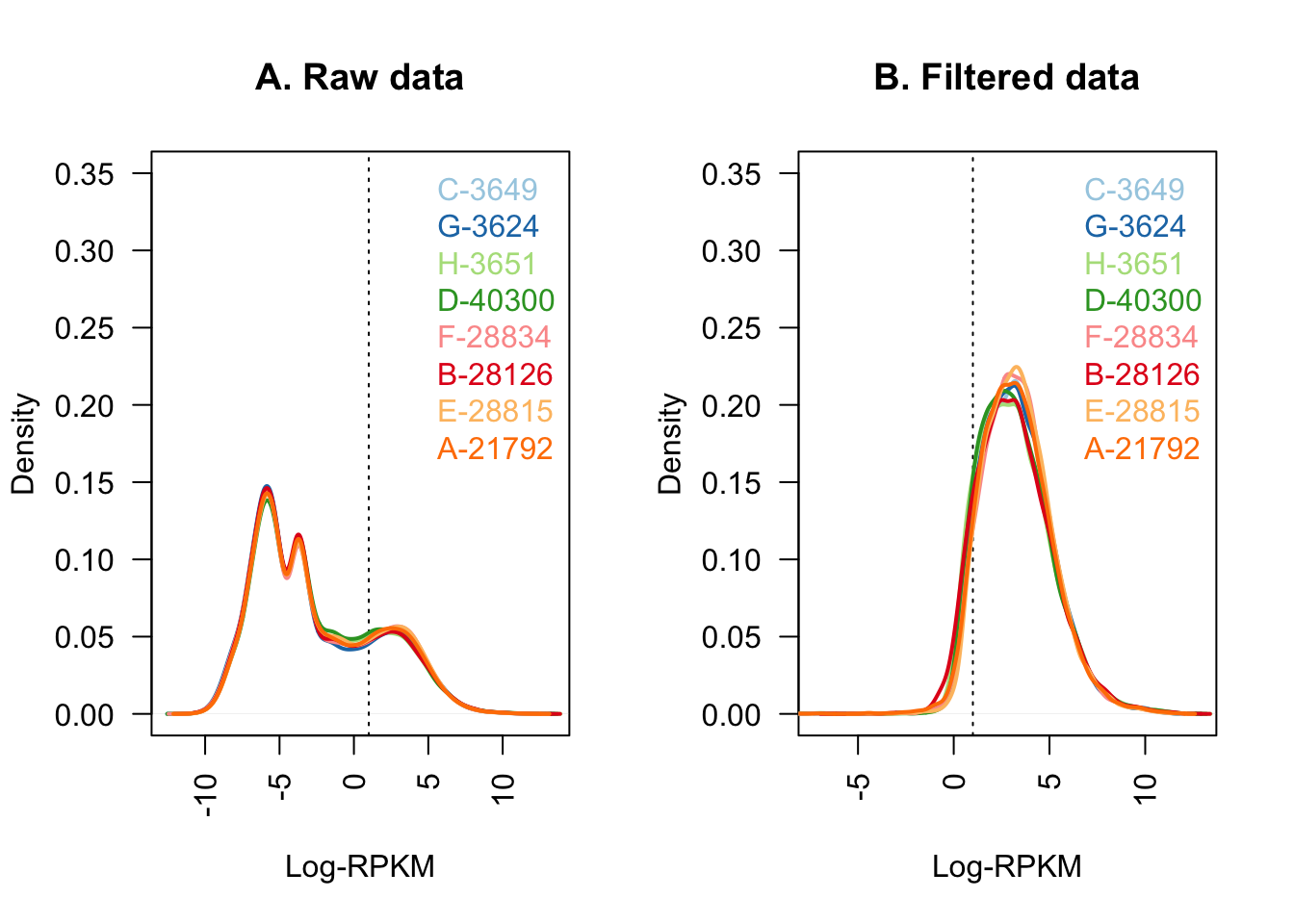
#Quick visualization of the normalization on the whole set of genes.
col <- brewer.pal(8, "Paired")
raw <- as.data.frame(dge$E[,1:8])
normed <- as.data.frame(dge_norm$E[,1:8])
par(mfrow=c(1,2))
boxplot(raw, las=2, col=col, main="")
title(main="Unnormalized data",ylab="Log-RPKM")
boxplot(normed, las=2, col=col, main="")
title(main="Normalized data",ylab="Log-RPKM")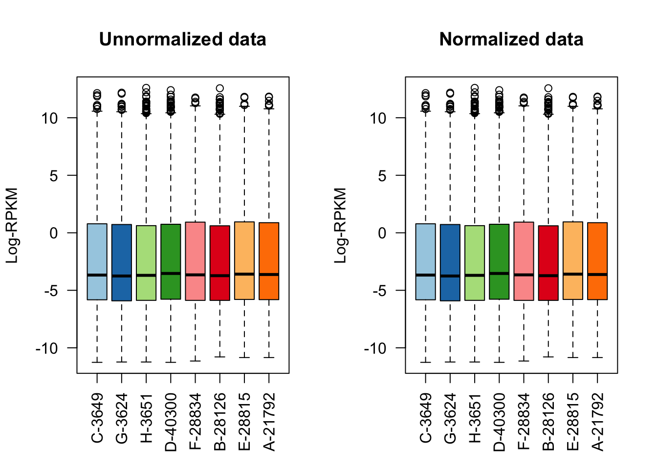
#Now, observe normalization on the filtered set of genes.
col <- brewer.pal(8, "Paired")
raw <- as.data.frame(dge_filt$E[,1:8])
normed <- as.data.frame(dge_final$E[,1:8])
par(mfrow=c(1,2))
boxplot(raw, las=2, col=col, main="")
title(main="Unnormalized data",ylab="Log-RPKM")
boxplot(normed, las=2, col=col, main="")
title(main="Normalized data",ylab="Log-RPKM")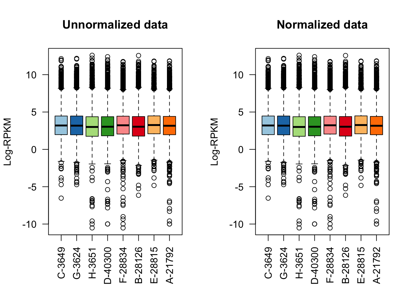
#Now, do some quick MDS plotting to make sure this expression data separates out species properly.
species <- c("C", "C", "C", "C", "H", "H", "H", "H")
color <- c(rep("red", 4), rep("blue", 4))
par(mfrow=c(1,1))
plotMDS(dge_final$E[,1:8], labels=species, col=color, main="MDS Plot") #Shows separation of the species along the logFC dimension representing the majority of the variance--orthogonal check to PCA, and looks great!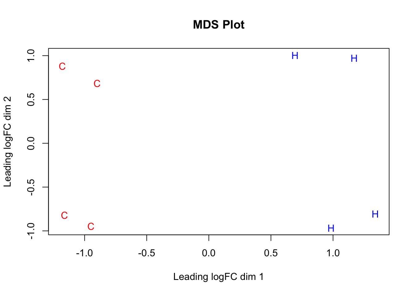
###Now, apply voom to get quality weights.
meta.exp.data <- data.frame("SP"=c("C", "C", "C", "C", "H", "H", "H", "H"), "SX"=c("M","M" ,"F","F","F", "M","M","F"))
SP <- factor(meta.exp.data$SP,levels = c("H","C"))
exp.design <- model.matrix(~0+SP)#(~1+meta.exp.data$SP+meta.exp.data$SX)
colnames(exp.design) <- c("Human", "Chimp")
weighted.data <- voom(dge_final, exp.design, plot=TRUE, normalize.method = "cyclicloess")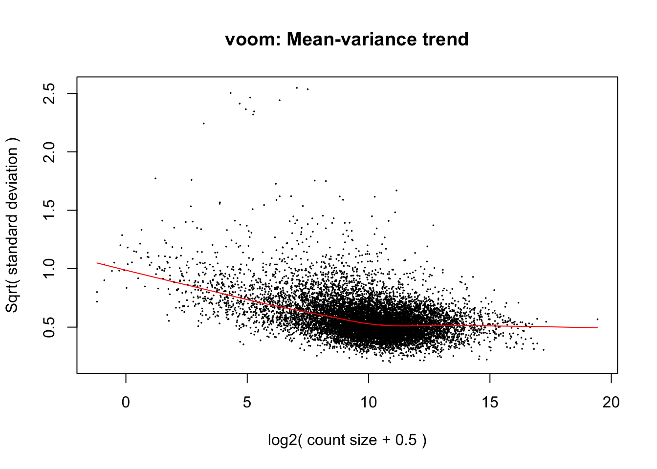
##Obtain rest of LM results, with particular eye to DE table!
vfit <- lmFit(weighted.data, exp.design)
efit <- eBayes(vfit)

mycon <- makeContrasts(HvC = Human-Chimp, levels = exp.design)
diff_species <- contrasts.fit(efit, mycon)
finalfit <- eBayes(diff_species)
detable <- topTable(finalfit, coef = 1, adjust.method = "BH", number = Inf, sort.by="none")
plotSA(efit, main="Final model: Mean−variance trend")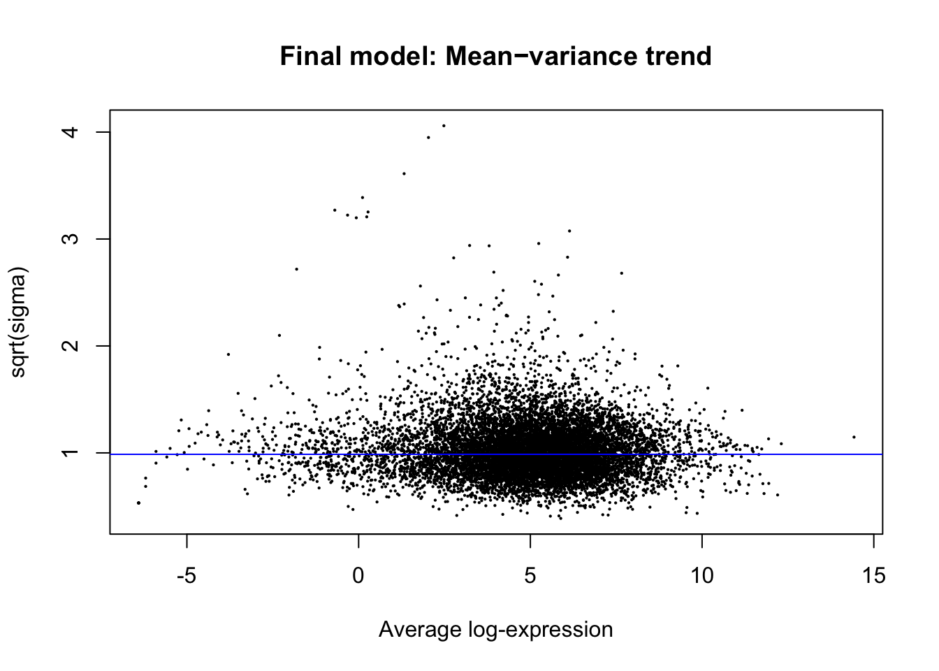
#Get lists of the DE and non-DE genes so I can run separate analyses on them at any point.
DEgenes <- detable$genes[which(detable$adj.P.Val<=0.05)]
nonDEgenes <- detable$genes[-which(detable$adj.P.Val<=0.05)]

#Rearrange RPKM and weight columns in voom object to be similar to the rest of my setup throughout in other dataframes.
weighted.data$E <- weighted.data$E[,c(8, 6, 1, 4, 7, 5, 2, 3)]
weighted.data$weights <- weighted.data$weights[,c(8, 6, 1, 4, 7, 5, 2, 3)]
RPKM <- weighted.data$E
rownames(RPKM) <- NULL #Just to match what I had before on midway2, about to write this out.
saveRDS(RPKM, file="output/IEE.RPKM.RDS")
saveRDS(weighted.data, file="output/IEE_voom_object.RDS") #write this object out, can then be read in with readRDS.
Overlap Between Hi-C Data and Orthogonal Gene Expression Data
In this section I find the overlap between the final filtered set of Hi-C significant hits and genes picked up on by an orthogonal RNA-seq experiment in the same set of cell lines. I utilize an in-house curated set of orthologous genes between humans and chimpanzees. Given that the resolution of the data is 10kb, I choose a simple and conservative approach and use a 1-nucleotide interval at the start of each gene as a proxy for the promoter. I then take a conservative pass and only use genes that had direct overlap with a bin from the Hi-C significant hits data, with more motivation explained below.
#Now, read in filtered data from linear_modeling_QC.Rmd.
data.filtered <- fread("output/data.4.filtered.lm.QC", header=TRUE, data.table=FALSE, stringsAsFactors = FALSE, showProgress=FALSE)
meta.data <- data.frame("SP"=c("H", "H", "C", "C", "H", "H", "C", "C"), "SX"=c("F", "M", "M", "F", "M", "F", "M", "F"), "Batch"=c(1, 1, 1, 1, 2, 2, 2, 2))

#TABLES1
#Write out data.filtered regions that are DC for supplementary table:
TABLES1 <- select(data.filtered, H1, H2, C1, C2, sp_BH_pval, sp_beta) %>% filter(., sp_BH_pval<=0.05)
TABLES1$Hchr <- gsub("-.*", "", TABLES1$H1)
TABLES1$H1start <- as.numeric(gsub(".*-", "", TABLES1$H1))
TABLES1$H1end <- TABLES1$H1start+10000
TABLES1$H2start <- as.numeric(gsub(".*-", "", TABLES1$H2))
TABLES1$H2end <- TABLES1$H2start+10000
TABLES1$Cchr <- gsub("-.*", "", TABLES1$C1)
TABLES1$C1start <- as.numeric(gsub(".*-", "", TABLES1$C1))
TABLES1$C1end <- TABLES1$C1start+10000
TABLES1$C2start <- as.numeric(gsub(".*-", "", TABLES1$C2))
TABLES1$C2end <- TABLES1$C2start+10000

select(TABLES1, Hchr, H1start, H1end, H2start, H2end, Cchr, C1start, C1end, C2start, C2end, sp_BH_pval, sp_beta) -> TABLES1
fwrite(TABLES1, "output/DC_regions.txt", col.names = TRUE, row.names = FALSE, sep = "\t")

#####GENE Hi-C Hit overlap: First, I obtain and rearrange the necessary files to get genes from both species and their overlaps with Hi-C bins.
#Read in necessary files: human and chimp orthologous genes from the meta ortho exon trios file. Then rearrange the columns of humgenes and chimpgenes to use group_by on them.
humgenes <- fread("data/Human_orthoexon_extended_info.txt", stringsAsFactors = FALSE, header=TRUE, data.table=FALSE)
chimpgenes <- fread("data/Chimp_orthoexon_extended_info.txt", stringsAsFactors = FALSE, header=TRUE, data.table=FALSE)
humgenes <- as.data.frame(humgenes[,c(1,5:8)])
chimpgenes <- as.data.frame(chimpgenes[,c(1,5:8)])
colnames(humgenes) <- c("genes", "Hchr", "Hstart", "Hend", "Hstrand")
colnames(chimpgenes) <- c("genes", "Cchr", "Cstart", "Cend", "Cstrand")
humgenes$Hchr <- paste("chr", humgenes$Hchr, sep="") #All properly formatted now!

#Bedtools groupby appears to have not worked properly to create files of single TSSs for genes from the meta ortho exons file, but this totally does! I've also utilized dplyr's group_by on the original file as well to ensure the same results. Now just making gene BED files that are 1-nt overlap at the very beginning of the first exon. Since I maintain strand information and will utilize it in bedtools closest-to, I am not concerned about whether the nt overlap goes the right direction or not. Note that if plyr is accidentally loaded AFTER dplyr, this will have issues (periods added at the end of start coords):
group_by(humgenes, genes) %>% summarise(Hchr=unique(Hchr), Hstart=as.numeric(min(Hstart)), Hstrand=unique(Hstrand)) -> humgenes
group_by(chimpgenes, genes) %>% summarise(Cchr=unique(Cchr), Cstart=min(Cstart), Cstrand=unique(Cstrand)) -> chimpgenes

#Quickly create a bed file to extract the genes that may overlap the region I'm pulling out for the paper example (chr5:147210000:147750000)
options(scipen = 999)
mytest <- filter(humgenes, Hchr=="chr5")
mytest <- mytest[(mytest$genes %in% weighted.data$genes$genes),]
mean.species.expression <- as.data.frame(weighted.data$E) #Now, need to pull out the mean expression values for all those genes!
mean.species.expression$genes <- rownames(mean.species.expression)
mean.species.expression$Hmean <- rowMeans(mean.species.expression[,c(1:2,5:6)])
mean.species.expression$Cmean <- rowMeans(mean.species.expression[,c(3:4,7:8)])
mean.species.expression <- mean.species.expression[,(-1:-8)]

#Now, prep bed files from the filtered data for each bin, in order to run bedtools-closest on them with the human and chimp gene data. This is for getting each bin's proximity to TSS by overlapping with the dfs just made (humgenes and chimpgenes). In the end this set of bedfiles is fairly useless, because really it would be preferable to get rid of duplicates so that I can merely group_by on a given bin afterwards and left_join as necessary. So somewhat deprecated, but I keep it here still:
hbin1 <- data.frame(chr=data.filtered$Hchr, start=as.numeric(gsub("chr.*-", "", data.filtered$H1)), end=as.numeric(gsub("chr.*-", "", data.filtered$H1))+10000)
hbin2 <- data.frame(chr=data.filtered$Hchr, start=as.numeric(gsub("chr.*-", "", data.filtered$H2)), end=as.numeric(gsub("chr.*-", "", data.filtered$H2))+10000)
cbin1 <- data.frame(chr=data.filtered$Cchr, start=as.numeric(gsub("chr.*-", "", data.filtered$C1)), end=as.numeric(gsub("chr.*-", "", data.filtered$C1))+10000)
cbin2 <- data.frame(chr=data.filtered$Cchr, start=as.numeric(gsub("chr.*-", "", data.filtered$C2)), end=as.numeric(gsub("chr.*-", "", data.filtered$C2))+10000)

#In most analyses, it will make more sense to have a single bed file for both sets of bins, and remove all duplicates. I create that here:
hbins <- rbind(hbin1[!duplicated(hbin1),], hbin2[!duplicated(hbin2),])
hbins <- hbins[!duplicated(hbins),]
cbins <- rbind(cbin1[!duplicated(cbin1),], cbin2[!duplicated(cbin2),])
cbins <- cbins[!duplicated(cbins),]

#Now, write all of these files out for analysis with bedtools.
write.table(hbin1, "~/Desktop/Hi-C/gene_expression/10kb_filt_overlaps/unsorted/hbin1.bed", quote = FALSE, sep="\t", row.names = FALSE, col.names=FALSE)
write.table(hbin2, "~/Desktop/Hi-C/gene_expression/10kb_filt_overlaps/unsorted/hbin2.bed", quote = FALSE, sep="\t", row.names = FALSE, col.names=FALSE)
write.table(cbin1, "~/Desktop/Hi-C/gene_expression/10kb_filt_overlaps/unsorted/cbin1.bed", quote = FALSE, sep="\t", row.names = FALSE, col.names=FALSE)
write.table(cbin2, "~/Desktop/Hi-C/gene_expression/10kb_filt_overlaps/unsorted/cbin2.bed", quote = FALSE, sep="\t", row.names = FALSE, col.names=FALSE)
write.table(humgenes, "~/Desktop/Hi-C/gene_expression/10kb_filt_overlaps/unsorted/humgenes.bed", quote=FALSE, sep="\t", row.names=FALSE, col.names=FALSE)
write.table(chimpgenes, "~/Desktop/Hi-C/gene_expression/10kb_filt_overlaps/unsorted/chimpgenes.bed", quote=FALSE, sep="\t", row.names=FALSE, col.names=FALSE)
write.table(hbins, "~/Desktop/Hi-C/gene_expression/10kb_filt_overlaps/unsorted/hbins.bed", quote=FALSE, sep="\t", row.names=FALSE, col.names=FALSE)
write.table(cbins, "~/Desktop/Hi-C/gene_expression/10kb_filt_overlaps/unsorted/cbins.bed", quote=FALSE, sep="\t", row.names=FALSE, col.names=FALSE)
options(scipen=0)

#Read in new, simpler bedtools closest files for genes. This is after running two commands, after sorting the files w/ sort -k1,1 -k2,2n in.bed > out.bed:
#bedtools closest -D a -a cgenes.sorted.bed -b cbins.sorted.bed > cgene.hic.overlap
#bedtools closest -D a -a hgenes.sorted.bed -b hbins.sorted.bed > hgene.hic.overlap
hgene.hic <- fread("~/Desktop/Hi-C/gene_expression/10kb_filt_overlaps/hgene.hic.overlap", header=FALSE, stringsAsFactors = FALSE, data.table=FALSE)
cgene.hic <- fread("~/Desktop/Hi-C/gene_expression/10kb_filt_overlaps/cgene.hic.overlap", header=FALSE, stringsAsFactors = FALSE, data.table=FALSE)


#Visualize the overlap of genes with bins and see how many genes we get back!
hum.genelap <- data.frame(overlap=seq(0, 100000, 1000), perc.genes = NA, tot.genes=NA)
for(row in 1:nrow(hum.genelap)){
  hum.genelap$perc.genes[row] <- sum(abs(hgene.hic$V10)<=hum.genelap$overlap[row])/length(hgene.hic$V10)
  hum.genelap$tot.genes[row] <- sum(abs(hgene.hic$V10)<=hum.genelap$overlap[row])
}

c.genelap <- data.frame(overlap=seq(0, 100000, 1000), perc.genes=NA, tot.genes=NA)
for(row in 1:nrow(c.genelap)){
  c.genelap$perc.genes[row] <- sum(abs(cgene.hic$V10)<=c.genelap$overlap[row])/length(cgene.hic$V10)
  c.genelap$tot.genes[row] <- sum(abs(cgene.hic$V10)<=c.genelap$overlap[row])
}
c.genelap$type <- "chimp"
hum.genelap$type <- "human"

#Examine what the potential gains are here if we are more lenient about the overlap/closeness to a TSS...
ggoverlap <- rbind(hum.genelap, c.genelap)
ggplot(data=ggoverlap) + geom_line(aes(x=overlap, y=perc.genes*100, color=type)) + ggtitle("Percent of Total Genes Picked Up | Min. Distance from TSS") + xlab("Distance from TSS") + ylab("Percentage of genes in ortho exon trios file (~44k)") + scale_color_discrete(guide=guide_legend(title="Species")) + coord_cartesian(xlim=c(0, 30000)) + scale_x_continuous(breaks=seq(0, 30000, 5000))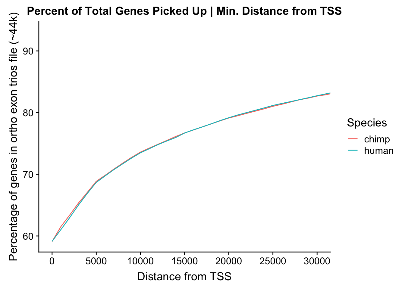
ggplot(data=ggoverlap) + geom_line(aes(x=overlap, y=tot.genes, color=type)) + ggtitle("Total # Genes Picked Up | Min. Distance from TSS") + xlab("Distance from TSS") + ylab("Total # of Genes Picked up On (of ~44k)") + scale_color_discrete(guide=guide_legend(title="Species")) + coord_cartesian(xlim=c(0, 30000)) + scale_x_continuous(breaks=seq(0, 30000, 5000))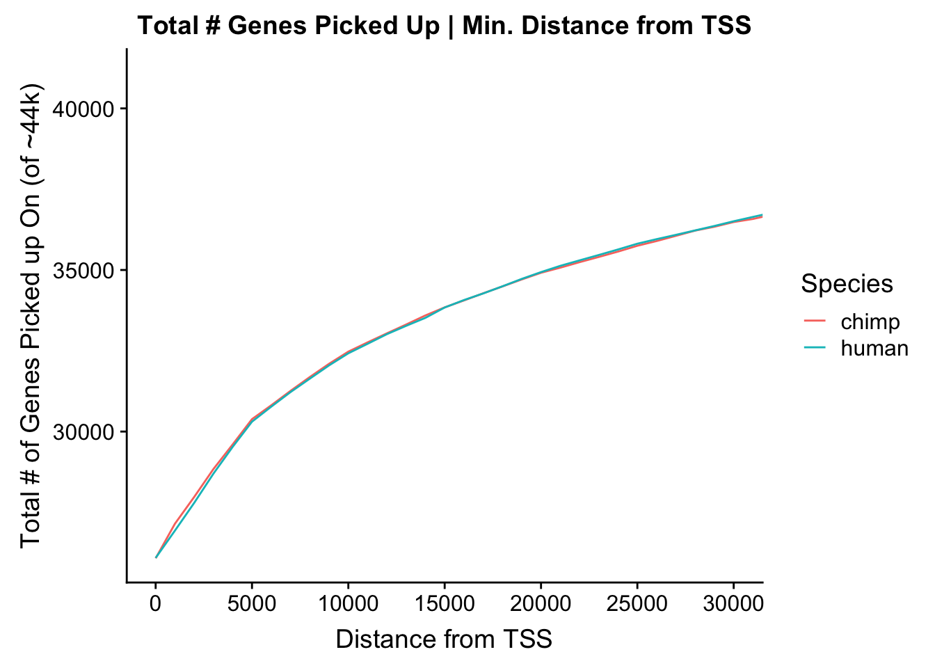
#Start with a conservative pass--only take those genes that had an actual overlap with a bin, not ones that were merely close to one. Allowing some leeway to include genes that are within 1kb, 2kb, 3kb etc. of a Hi-C bin adds an average of ~800 genes per 1kb. We can also examine the distribution manually to motivate this decision:
quantile(abs(hgene.hic$V10), probs=seq(0, 1, 0.025))
0% 2.5% 5% 7.5% 10% 12.5% 15%
0.0 0.0 0.0 0.0 0.0 0.0 0.0
17.5% 20% 22.5% 25% 27.5% 30% 32.5%
0.0 0.0 0.0 0.0 0.0 0.0 0.0
35% 37.5% 40% 42.5% 45% 47.5% 50%
0.0 0.0 0.0 0.0 0.0 0.0 0.0
52.5% 55% 57.5% 60% 62.5% 65% 67.5%
0.0 0.0 0.0 435.4 1741.0 2968.2 4324.0
70% 72.5% 75% 77.5% 80% 82.5% 85%
6226.2 8868.0 12336.0 16610.0 22034.4 29271.5 38300.2
87.5% 90% 92.5% 95% 97.5% 100%
50248.0 67698.4 92599.2 135125.0 243068.9 7581822.0 quantile(abs(cgene.hic$V10), probs=seq(0, 1, 0.025)) 0% 2.5% 5% 7.5% 10% 12.5%
0.0 0.0 0.0 0.0 0.0 0.0
15% 17.5% 20% 22.5% 25% 27.5%
0.0 0.0 0.0 0.0 0.0 0.0
30% 32.5% 35% 37.5% 40% 42.5%
0.0 0.0 0.0 0.0 0.0 0.0
45% 47.5% 50% 52.5% 55% 57.5%
0.0 0.0 0.0 0.0 0.0 0.0
60% 62.5% 65% 67.5% 70% 72.5%
237.4 1507.0 2800.0 4237.4 6125.6 8750.4
75% 77.5% 80% 82.5% 85% 87.5%
12181.0 16648.0 22317.4 29420.0 38490.0 50656.0
90% 92.5% 95% 97.5% 100%
67470.4 92415.3 136417.4 243285.0 21022081.0 #Note I looked at proportion of overlap with DE and with non-DE genes just for curiosity, and roughly 66% of the DE genes have overlap with a Hi-C bin while roughly 70% of the non-DE genes do. Since this result isn't particularly interesting I have collapsed that analysis here.
#Also are interested in seeing how this differs for DE and non-DE genes.
dehgene.hic <- hgene.hic[which(hgene.hic$V4 %in% DEgenes),]
decgene.hic <- cgene.hic[which(cgene.hic$V4 %in% DEgenes),]
nondehgene.hic <- hgene.hic[which(hgene.hic$V4 %in% nonDEgenes),]
nondecgene.hic <- cgene.hic[which(cgene.hic$V4 %in% nonDEgenes),]
sum(dehgene.hic$V10==0)[1] 1538sum(nondehgene.hic$V10==0)[1] 6231quantile(abs(dehgene.hic$V10), probs=seq(0, 1, 0.025)) 0% 2.5% 5% 7.5% 10% 12.5%
0.00 0.00 0.00 0.00 0.00 0.00
15% 17.5% 20% 22.5% 25% 27.5%
0.00 0.00 0.00 0.00 0.00 0.00
30% 32.5% 35% 37.5% 40% 42.5%
0.00 0.00 0.00 0.00 0.00 0.00
45% 47.5% 50% 52.5% 55% 57.5%
0.00 0.00 0.00 0.00 0.00 0.00
60% 62.5% 65% 67.5% 70% 72.5%
0.00 0.00 0.00 0.00 1061.10 2339.00
75% 77.5% 80% 82.5% 85% 87.5%
3465.25 4832.80 6883.20 10197.35 14622.95 20465.88
90% 92.5% 95% 97.5% 100%
30342.90 44341.90 65604.90 129936.58 5262467.00 quantile(abs(nondehgene.hic$V10), probs=seq(0, 1, 0.025)) 0% 2.5% 5% 7.5% 10% 12.5%
0.000 0.000 0.000 0.000 0.000 0.000
15% 17.5% 20% 22.5% 25% 27.5%
0.000 0.000 0.000 0.000 0.000 0.000
30% 32.5% 35% 37.5% 40% 42.5%
0.000 0.000 0.000 0.000 0.000 0.000
45% 47.5% 50% 52.5% 55% 57.5%
0.000 0.000 0.000 0.000 0.000 0.000
60% 62.5% 65% 67.5% 70% 72.5%
0.000 0.000 0.000 0.000 0.000 813.875
75% 77.5% 80% 82.5% 85% 87.5%
2008.500 3090.750 4453.000 6491.250 10166.000 15596.750
90% 92.5% 95% 97.5% 100%
23375.000 35249.500 54960.750 104309.875 6845725.000 And we can see that the majority of the genes (57.5%) have direct overlap with a bin. I’ll thus start with one very conservative set with only genes that have direct overlap with a bin. Later I may return to this and add and another slightly more lenient bin capturing ~10% more of the genes by allowing +/- 5kb of wiggle room.
Linear Modeling Annotation
In this next section I simply add information obtained from linear modeling on the Hi-C interaction frequencies to the appropriate genes having overlap with Hi-C bins. Because one Hi-C bin frequently shows up many times in the data, this means I must choose some kind of summary for Hi-C contact frequencies and linear modeling annotations for each gene. I toy with a variety of these summaries here, including choosing the minimum FDR contact, the maximum beta contact, the upstream contact, or summarizing all a bin’s contacts with the weighted Z-combine method or median FDR values.
hgene.hic.overlap <- filter(hgene.hic, V10==0) #Still leaves a solid ~26k genes.
cgene.hic.overlap <- filter(cgene.hic, V10==0) #Still leaves a solid ~26k genes.

#Add a column to both dfs indicating where along a bin the gene in question is found (from 0-10k):
hgene.hic.overlap$bin_pos <- abs(hgene.hic.overlap$V8-hgene.hic.overlap$V2)
cgene.hic.overlap$bin_pos <- abs(cgene.hic.overlap$V8-cgene.hic.overlap$V2)

#Rearrange columns and create another column of the bin ID.
hgene.hic.overlap <- hgene.hic.overlap[,c(4, 7:9, 6, 11, 1:2)]
hgene.hic.overlap$HID <- paste(hgene.hic.overlap$V7, hgene.hic.overlap$V8, sep="-")
cgene.hic.overlap <- cgene.hic.overlap[,c(4, 7:9, 6, 11, 1:2)]
cgene.hic.overlap$CID <- paste(cgene.hic.overlap$V7, cgene.hic.overlap$V8, sep="-")
colnames(hgene.hic.overlap) <- c("genes", "HiC_chr", "H1start", "H1end", "Hstrand", "bin_pos", "genechr", "genepos", "HID")
colnames(cgene.hic.overlap) <- c("genes", "HiC_chr", "C1start", "C1end", "Cstrand", "bin_pos", "genechr", "genepos", "CID")
#Gets me an hfinal table with a lot of the information concatenated together--now need the same thing for chimps, only to get the n contacts (since this could differ!)
hbindf <- select(data.filtered, "H1", "H2", "ALLvar", "SE", "sp_beta", "sp_pval", "sp_BH_pval", "Hdist")
names(hbindf) <- c("HID", "HID2", "ALLvar", "SE", "sp_beta", "sp_pval", "sp_BH_pval", "distance") #I have confirmed that all the HID2s are higher numbered coordinates than the HID1s, the only instance in which this isn't the case is when the two bins are identical (this should have been filtered out long before now).

hbindf <- hbindf[(which(hbindf$dist!=0)),] #Removes pairs where the same bin represents both mates. These instances occur exclusively when liftOver of the genomic coordinates from one species to another, and the subsequent rounding to the nearest 10kb, results in a contact between adjacent bins in one species being mapped as a contact between the same bin in the other species. Because there are less than 50 instances of this total in the dataset I simply remove it here without further worry.

#Remembering that all the first mates in the pair are lower coordinates than the second mates:
#This works for getting the FDR of closest downstream hits for the first column. Technically this would also make these the closest upstream hits for any bins that are UNIQUE and NOT REPEATED to the second column. For unique bins in this column, they have no upstream hits, and this gets their downstream hits. I can do the same thing but on the second set of IDs to get the potential upstream hits for any bins, then do a full_join on the two to get everything! Many of these metrics need to be done on a duplicated df to ensure I have all copies of a bin in one column, but the upstream and downstream analyses need to be run separately.
group_by(hbindf, HID) %>% summarise(DS_bin=HID2[which.min(distance)], DS_FDR=sp_BH_pval[which.min(distance)], DS_dist=distance[which.min(distance)]) -> hbin1.downstream

group_by(hbindf, HID2) %>% summarise(US_bin=HID[which.min(distance)], US_FDR=sp_BH_pval[which.min(distance)], US_dist=distance[which.min(distance)]) -> hbin2.upstream
colnames(hbin2.upstream) <- c("HID", "US_bin", "US_FDR", "US_dist")

Hstreams <- full_join(hbin1.downstream, hbin2.upstream, by="HID")

#Now, need to create a df with all the hits duplicated (but columns reversed) to account for duplicated bins in each column. This is better for any analysis that shares information across the interactions (minimums, sums, means, medians, etc.)
hbindf.flip <- hbindf[,c(2, 1, 3:7)]
colnames(hbindf.flip)[1:2] <- c("HID", "HID2")
hbindf_x2 <- rbind(hbindf[,1:7], hbindf.flip) #It's worth noting that a version of this with duplicates removed would be very useful for enrichment analyses...

#Now, use group_by from dplyr to combine information for a given bin across all its Hi-C contacts. Here I'll be pulling out contact, p-value, and bin with minimum FDR, its beta; the median FDR; the maximum beta and its FDR and bin; and a weighted combination method for p-values for species from linear modeling. This is based off of (http://onlinelibrary.wiley.com/doi/10.1111/j.1420-9101.2005.00917.x/full) under the assumption $s2.post is the actual error variance. (forthcoming)
group_by(hbindf_x2, HID) %>% summarise(min_FDR_bin=HID2[which.min(sp_BH_pval)], min_FDR=min(sp_BH_pval), min_FDR_pval=sp_pval[which.min(sp_BH_pval)], min_FDR_B=sp_beta[which.min(sp_BH_pval)], median_FDR=median(sp_BH_pval),  weighted_Z.ALLvar=pnorm((sum((1/ALLvar)*((qnorm(1-sp_pval))))/sqrt(sum((1/ALLvar)^2))), lower.tail=FALSE), weighted_Z.s2post=pnorm(sum((1/(SE^2))*qnorm(1-sp_pval))/sqrt(sum(1/SE^2)), lower.tail=FALSE), fisher=-2*sum(log(sp_pval)), numcontacts=n(), max_B_bin=HID2[which.max(abs(sp_beta))], max_B_FDR=sp_BH_pval[which.max(abs(sp_beta))], max_B=sp_beta[which.max(abs(sp_beta))]) -> hbin.info

#Now, full_join the hbin.info and Hstreams dfs, incorporating all the information about the hbins in my data:
full_join(hbin.info, Hstreams, by="HID") -> hbin.full.info

#Now I combine the gene overlap tables and the full information tables for the human genes and bins!
left_join(hgene.hic.overlap, hbin.full.info, by="HID") -> humgenes.hic.full
colnames(humgenes.hic.full)[1:5] <- c("genes", "Hchr", "Hstart", "Hend", "Hstrand") #Fix column names for what was just created

###Now, do the whole thing over again for chimps, and then combine with the human gene overlap before joining on detable!
#Gets me a cfinal table with a lot of the information concatenated together.
cbindf <- select(data.filtered, "C1", "C2", "ALLvar", "SE", "sp_beta", "sp_pval", "sp_BH_pval", "Cdist") #Pulling out cols C1, C2, ALLvar, SE, sp_beta, sp_pval, sp_BH_pval, and Cdist
names(cbindf) <- c("CID", "CID2", "ALLvar", "SE", "sp_beta", "sp_pval", "sp_BH_pval", "distance") #I have confirmed that all the CID2s are higher numbered coordinates than the CID1s, the only instance in which this isn't the case is when the two bins are identical (this should have been filtered out long before now).

cbindf <- cbindf[(which(cbindf$dist!=0)),] #Removes rows from the cbindf that REALLY shouldn't be there to begin with. There are ~620 hits like this.

#Remembering that all the first mates in the pair are lower coordinates than the second mates:
#This works for getting the FDR of closest downstream hits for the first column. Technically this would also make these the closest upstream hits for any bins that are UNIQUE and NOT REPEATED to the second column. For unique bins in this column, they have no upstream hits, and this gets their downstream hits. I can do the same thing but on the second set of IDs to get the potential upstream hits for any bins, then do a full_join on the two to get everything! Many of these metrics need to be done on a duplicated df to ensure I have all copies of a bin in one column, but the upstream and downstream analyses need to be run separately.
group_by(cbindf, CID) %>% summarise(DS_bin=CID2[which.min(distance)], DS_FDR=sp_BH_pval[which.min(distance)], DS_dist=distance[which.min(distance)]) -> cbin1.downstream

group_by(cbindf, CID2) %>% summarise(US_bin=CID[which.min(distance)], US_FDR=sp_BH_pval[which.min(distance)], US_dist=distance[which.min(distance)]) -> cbin2.upstream
colnames(cbin2.upstream) <- c("CID", "US_bin", "US_FDR", "US_dist")

Cstreams <- full_join(cbin1.downstream, cbin2.upstream, by="CID")

#Now, need to create a df with all the hits duplicated (but columns reversed) to account for duplicated bins in each column. This is better for any analysis that shares information across the interactions (minimums, sums, means, medians, etc.)
cbindf.flip <- cbindf[,c(2, 1, 3:7)]
colnames(cbindf.flip)[1:2] <- c("CID", "CID2")
cbindf_x2 <- rbind(cbindf[,1:7], cbindf.flip)

#Group by again for chimp hits as was done for humans above.
group_by(cbindf_x2, CID) %>% summarise(min_FDR_bin=CID2[which.min(sp_BH_pval)], min_FDR=min(sp_BH_pval), min_FDR_B=sp_beta[which.min(sp_BH_pval)], median_FDR=median(sp_BH_pval), weighted_Z.ALLvar=pnorm((sum((1/ALLvar)*((qnorm(1-sp_pval))))/sqrt(sum((1/ALLvar)^2))), lower.tail=FALSE), weighted_Z.s2post=pnorm(sum((1/(SE^2))*qnorm(1-sp_pval))/sqrt(sum(1/SE^2)), lower.tail=FALSE), fisher=-2*sum(log(sp_pval)), numcontacts=n(), max_B_bin=CID2[which.max(abs(sp_beta))], max_B_FDR=sp_BH_pval[which.max(abs(sp_beta))], max_B=sp_beta[which.max(abs(sp_beta))]) -> cbin.info

#Now, full_join the cbin.info and Cstreams dfs, incorporating all the information about the cbins in my data:
full_join(cbin.info, Cstreams, by="CID") -> cbin.full.info

#Now I combine the gene overlap tables and the full information tables for the human genes and bins!
left_join(cgene.hic.overlap, cbin.full.info, by="CID") -> chimpgenes.hic.full
colnames(chimpgenes.hic.full)[1:5] <- c("genes", "Hchr", "Hstart", "Hend", "Hstrand") #Fix column names for what was just created

#Now, combine chimpgenes.hic.full and humgenes.hic.full before a final left_join on detable:
full_join(humgenes.hic.full, chimpgenes.hic.full, by="genes", suffix=c(".H", ".C")) -> genes.hic.info
left_join(detable, genes.hic.info, by="genes") -> gene.hic.overlap.info

#Clean this dataframe up, removing rows where there is absolutely no Hi-C information for the gene.
filt.indices <- rowSums(is.na(gene.hic.overlap.info)) #51 NA values are found when there is absolutely no Hi-C information.
filt.indices <- which(filt.indices==51)
gene.hic.filt <- gene.hic.overlap.info[-filt.indices,] #Still leaves a solid 8,174 genes. Note that I will have to choose human or chimp values here for many of these columns, as not all of the values are the same (and many are missing in one species relative to the other). In some cases, may be able to just take minimum or maximum value from either in order to get at what I want.
saveRDS(gene.hic.filt, "~/Desktop/Hi-C/gene.hic.filt.RDS")
Differential Expression-Differential Hi-C Enrichment Analyses
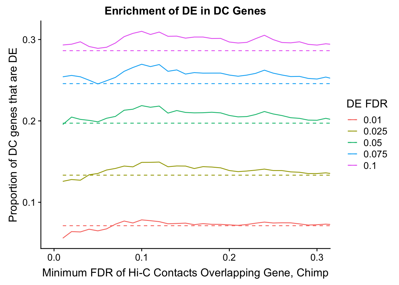
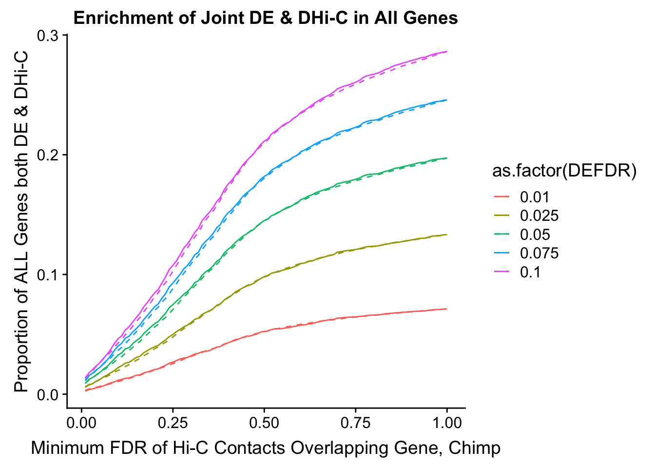
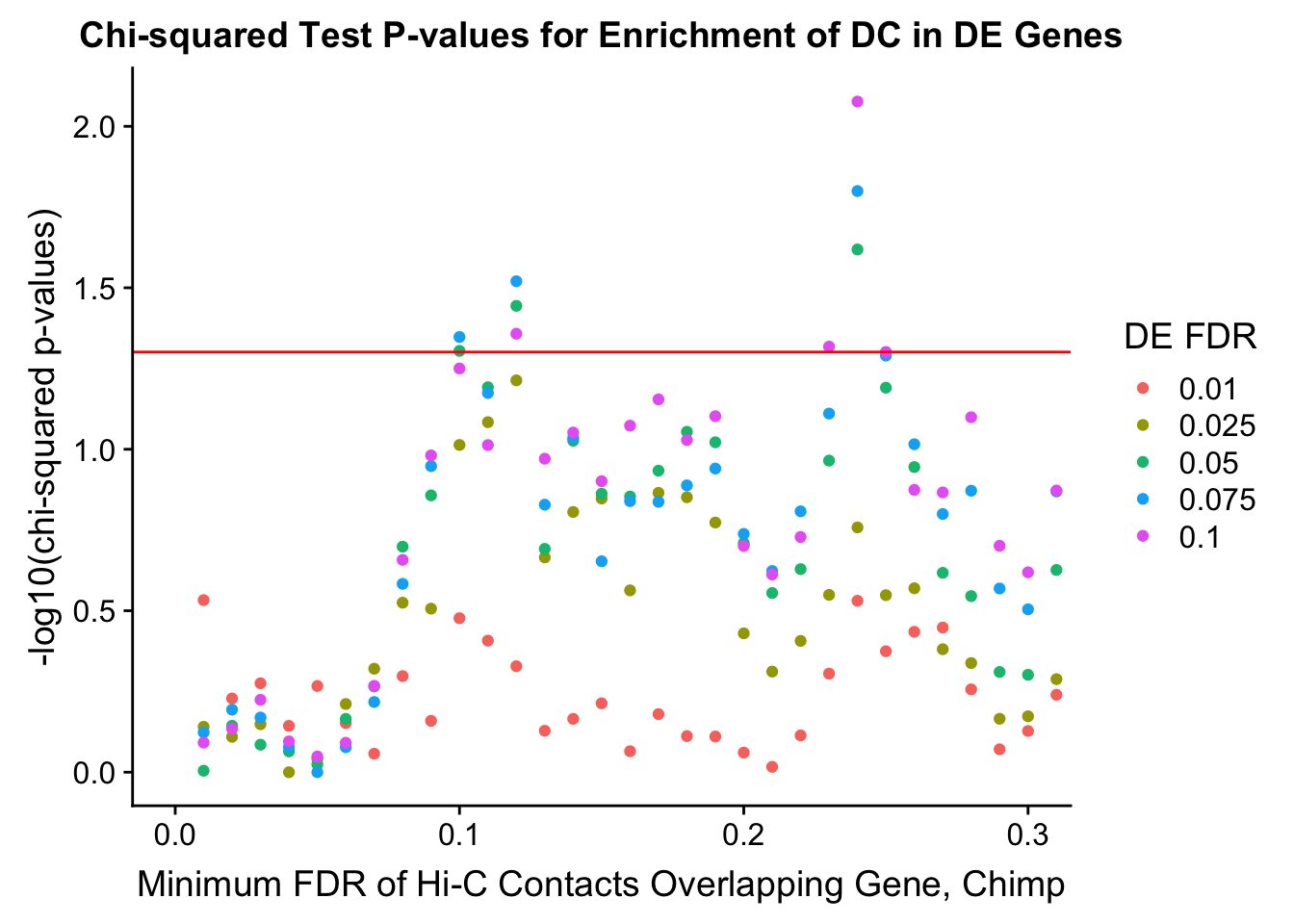
Now I look for enrichment of DHi-C in DE genes using a variety of different metrics to call DHi-C. I now look to see if genes that are differentially expressed are also differential in Hi-C contacts (DHi-C). That is to say, are differentially expressed genes enriched in their overlapping bins for Hi-C contacts that are also differential between the species? To do this I utilize p-values from my prior linear modeling as well as previous RNA-seq analysis. I construct a function to calculate proportions of DE and DHi-C genes, as well as a function to plot this out in a variety of different ways.
####Enrichment analyses!
#A function for calculating proportion of DE genes that are DHi-C under a variety of different paradigms. Accounts for when no genes are DHi-C and when all genes are DHi-C. Returns the proportion of DE genes that are also DHi-C, as well as the expected proportion based on conditional probability alone.
prop.calculator <- function(de.vec, hic.vec, i, k){
my.result <- data.frame(prop=NA, exp.prop=NA, chisq.p=NA, Dneither=NA, DE=NA, DHiC=NA, Dboth=NA)
bad.indices <- which(is.na(hic.vec)) #First obtain indices where Hi-C info is missing, if there are any, then remove from both vectors.
if(length(bad.indices>0)){
de.vec <- de.vec[-bad.indices]
hic.vec <- hic.vec[-bad.indices]}
de.vec <- ifelse(de.vec<=i, 1, 0)
hic.vec <- ifelse(hic.vec<=k, 1, 0)
if(sum(hic.vec, na.rm=TRUE)==0){#The case where no genes show up as DHi-C.
my.result[1,] <- c(0, 0, 0, sum(de.vec==0, na.rm=TRUE), sum(de.vec==1, na.rm=TRUE), 0, 0) #Since no genes are DHi-C, the proportion is 0 and our expectation is 0, set p-val=0 since it's irrelevant.
}
else if(sum(hic.vec)==length(hic.vec)){ #The case where every gene shows up as DHi-C
my.result[1,] <- c(1, 1, 0, 0, 0, sum(hic.vec==1&de.vec==0, na.rm = TRUE), sum(de.vec==1&hic.vec==1, na.rm=TRUE)) #If every gene is DHi-C, the observed proportion of DE genes DHi-C is 1, and the expected proportion of DE genes also DHi-C would also be 1 (all DE genes are DHi-C, since all genes are). Again set p-val to 0 since irrelevant comparison.
}
else{#The typical case, where we get an actual table
mytable <- table(as.data.frame(cbind(de.vec, hic.vec)))
my.result[1,1] <- mytable[2,2]/sum(mytable[2,]) #The observed proportion of DE genes that are also DHi-C. # that are both/total # DE
my.result[1,2] <- (((sum(mytable[2,])/sum(mytable))*((sum(mytable[,2])/sum(mytable))))*sum(mytable))/sum(mytable[2,]) #The expected proportion: (p(DE) * p(DHiC)) * total # genes / # DE genes
my.result[1,3] <- chisq.test(mytable)$p.value
my.result[1,4] <- mytable[1,1]
my.result[1,5] <- mytable[2,1]
my.result[1,6] <- mytable[1,2]
my.result[1,7] <- mytable[2,2]
}
return(my.result)
}
#This is a function that computes observed and expected proportions of DE and DHiC enrichments, and spits out a variety of different visualizations for them. As input it takes a dataframe, the names of its DHiC and DE p-value columns, and a name to represent the type of Hi-C contact summary for the gene that ends up on the x-axis of all the plots.
enrichment.plotter <- function(df, HiC_col, DE_col, xlab, xmax=0.3, i=c(0.01, 0.025, 0.05, 0.075, 0.1), k=seq(0.01, 1, 0.01)){
enrich.table <- data.frame(DEFDR = c(rep(i[1], 100), rep(i[2], 100), rep(i[3], 100), rep(i[4], 100), rep(i[5], 100)), DHICFDR=rep(k, 5), prop.obs=NA, prop.exp=NA, chisq.p=NA, Dneither=NA, DE=NA, DHiC=NA, Dboth=NA)
for(de.FDR in i){
for(hic.FDR in k){
enrich.table[which(enrich.table$DEFDR==de.FDR&enrich.table$DHICFDR==hic.FDR), 3:9] <- prop.calculator(df[,DE_col], df[,HiC_col], de.FDR, hic.FDR)
}
}
des.enriched <- ggplot(data=enrich.table, aes(x=DHICFDR, y=prop.obs, group=as.factor(DEFDR), color=as.factor(DEFDR))) +geom_line()+ geom_line(aes(y=prop.exp), linetype="dashed", size=0.5) + ggtitle("Enrichment of DC in DE Genes") + xlab(xlab) + ylab("Proportion of DE genes that are DC") + guides(color=guide_legend(title="FDR for DE Genes"))
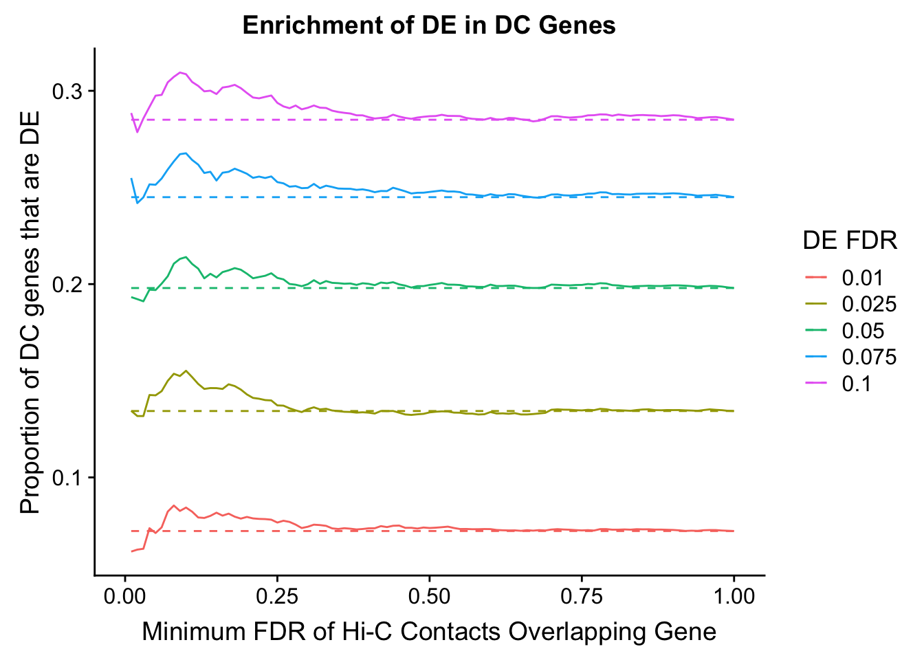
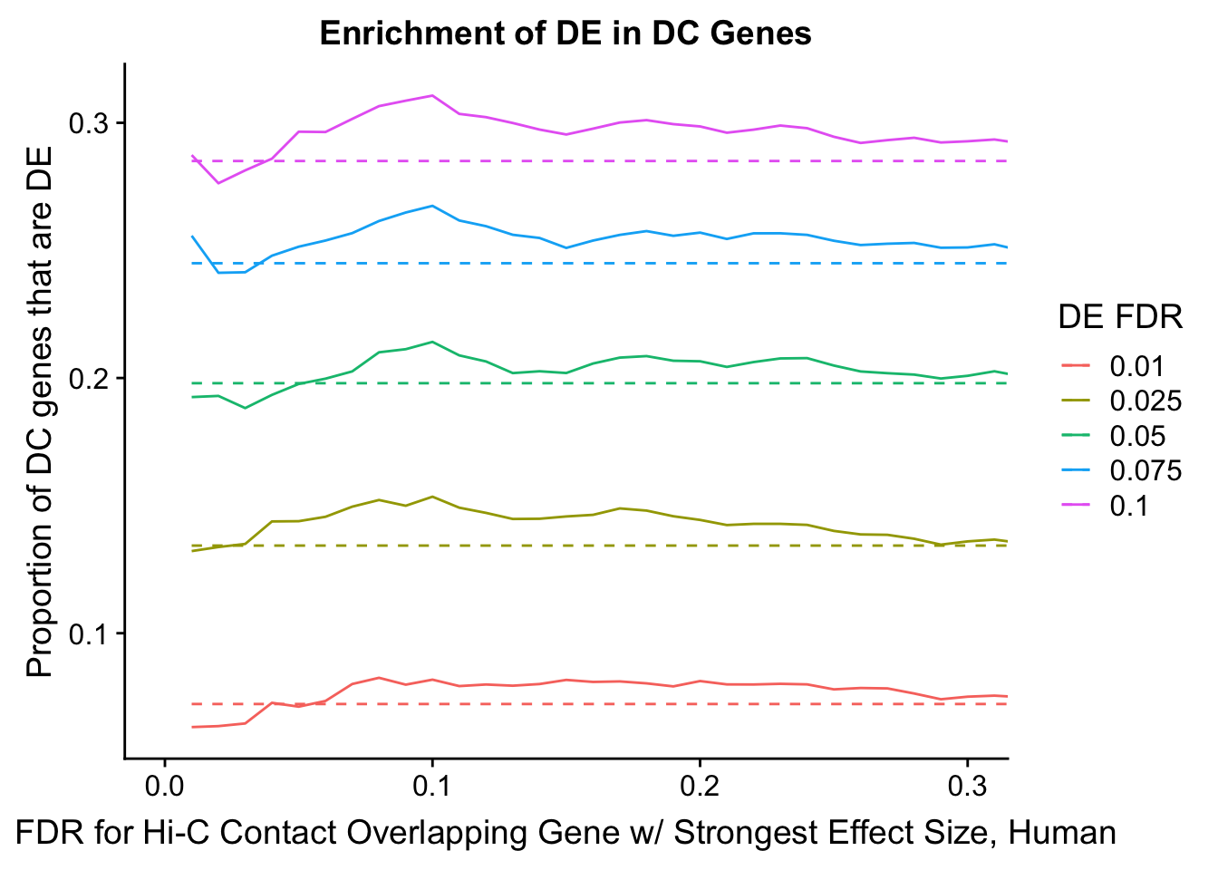
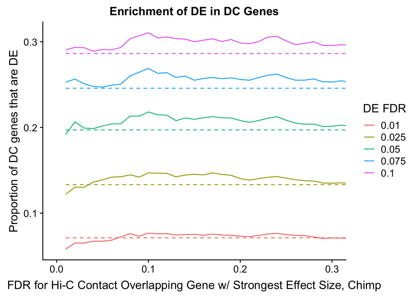
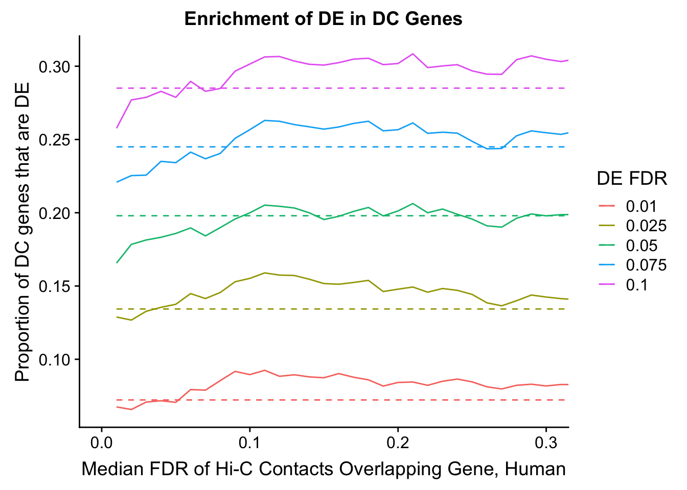
dhics.enriched <- ggplot(data=enrich.table, aes(x=DHICFDR, y=Dboth/(Dboth+DHiC), group=as.factor(DEFDR), color=as.factor(DEFDR))) + geom_line() + geom_line(aes(y=(((((DE+Dboth)/(Dneither+DE+DHiC+Dboth))*((DHiC+Dboth)/(Dneither+DE+DHiC+Dboth)))*(Dneither+DE+DHiC+Dboth))/(DHiC+Dboth))), linetype="dashed") + ylab("Proportion of DC genes that are DE") +xlab(xlab) + ggtitle("Enrichment of DE in DC Genes") + coord_cartesian(xlim=c(0, xmax)) + guides(color=guide_legend(title="DE FDR"))
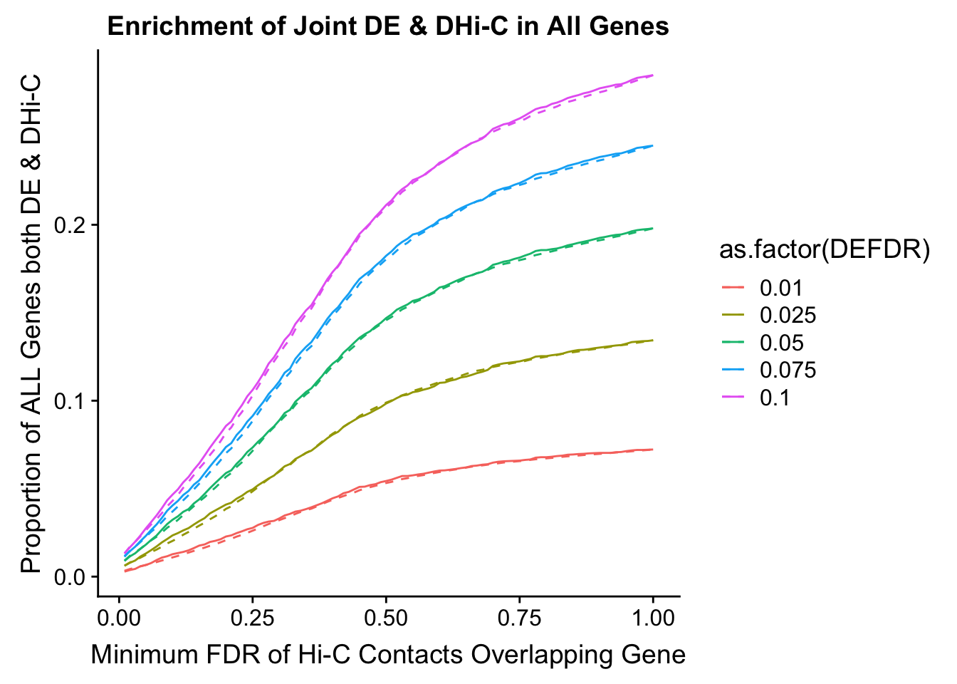
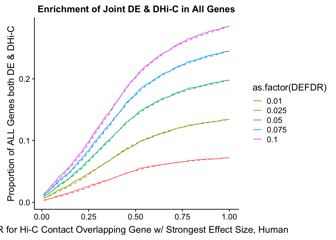
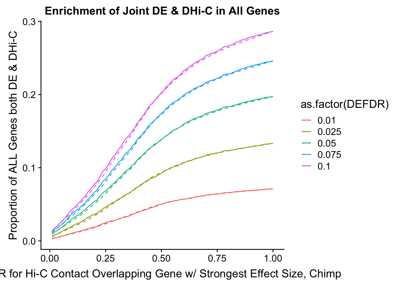
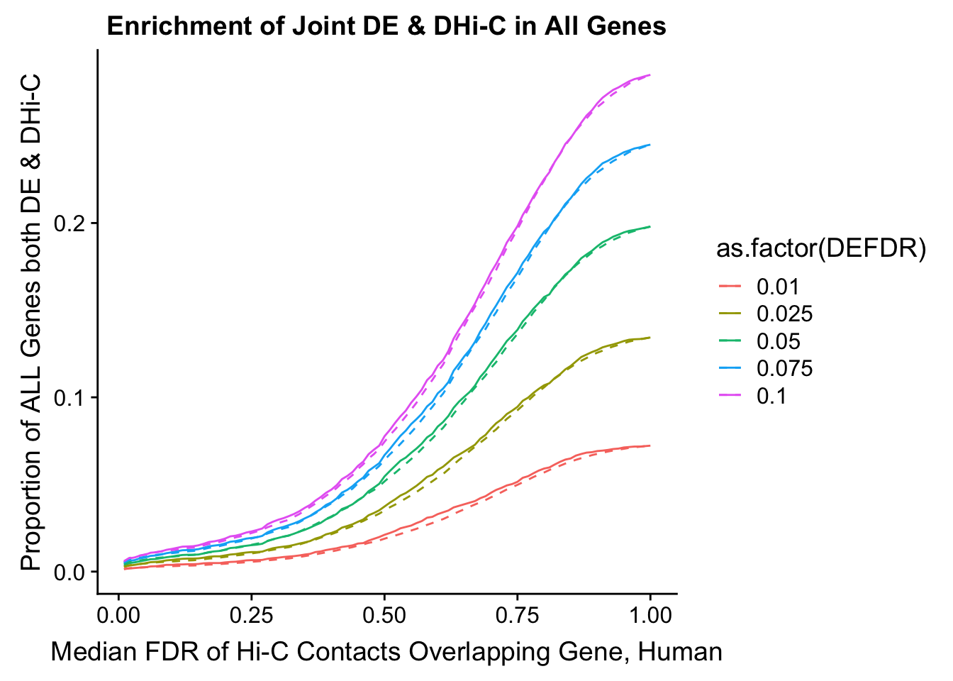
joint.enriched <- ggplot(data=enrich.table, aes(x=DHICFDR, y=Dboth/(Dneither+DE+DHiC+Dboth), group=as.factor(DEFDR), color=as.factor(DEFDR))) + geom_line() + ylab("Proportion of ALL Genes both DE & DHi-C") + xlab(xlab) + geom_line(aes(y=((DE+Dboth)/(Dneither+DE+DHiC+Dboth))*((DHiC+Dboth)/(Dneither+DE+DHiC+Dboth))), linetype="dashed") + ggtitle("Enrichment of Joint DE & DHi-C in All Genes")
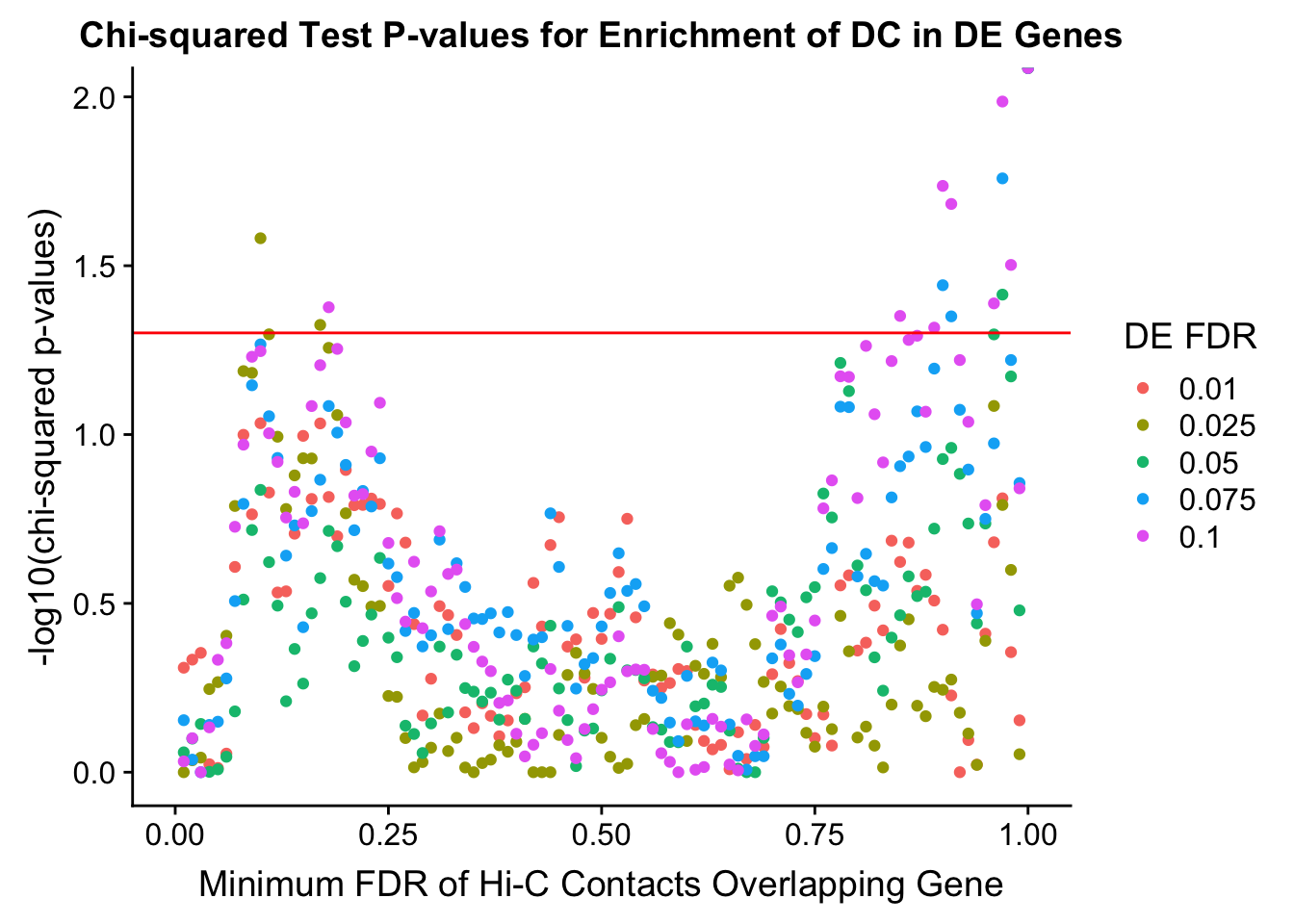
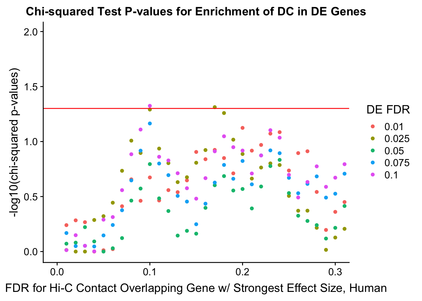
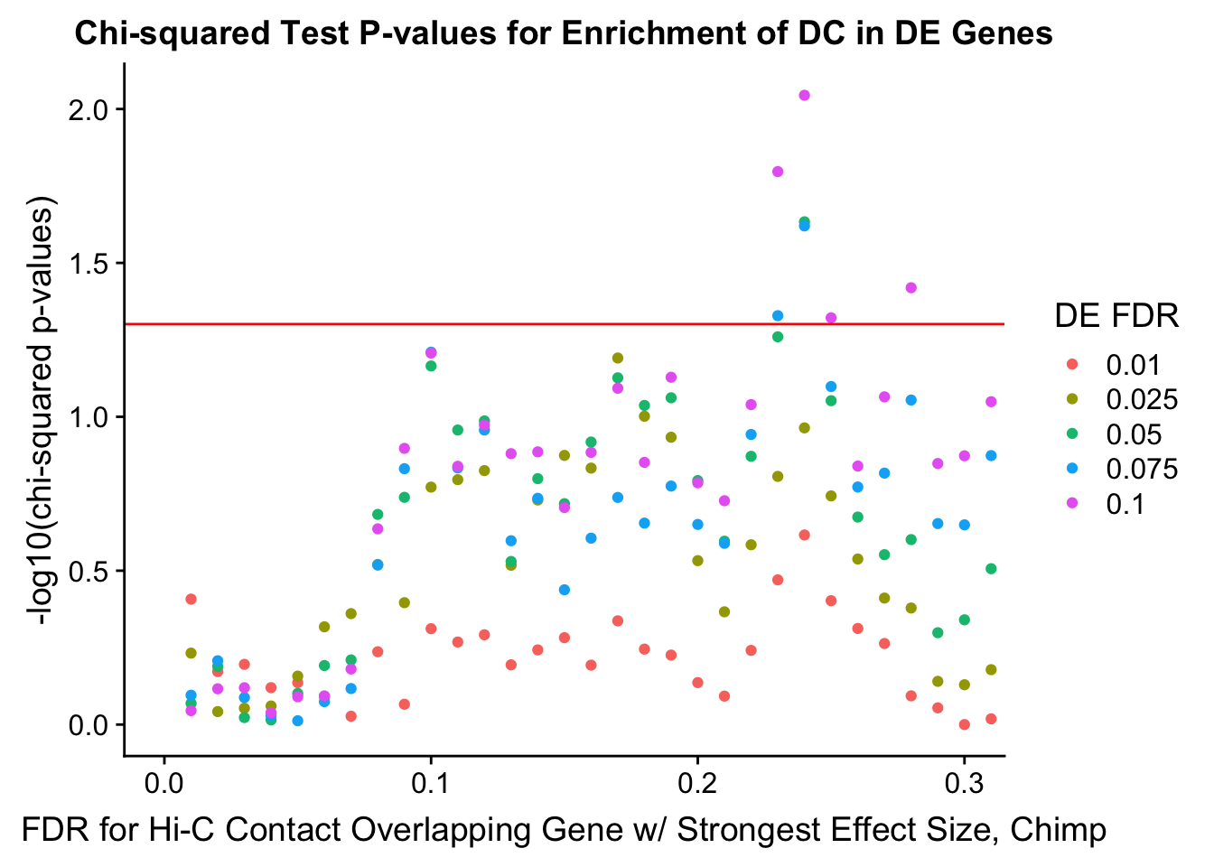
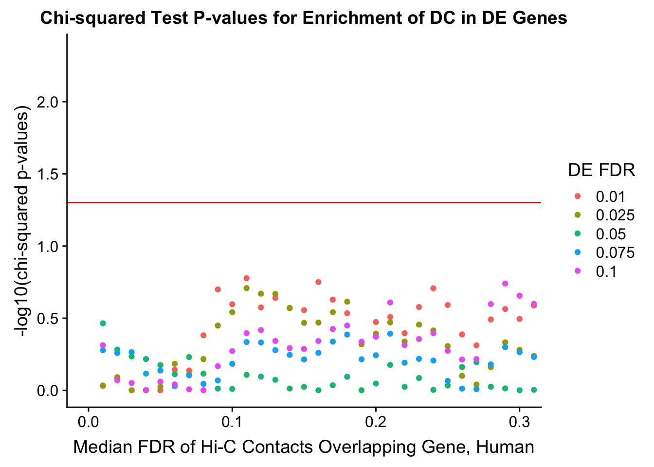
chisq.p <- ggplot(data=enrich.table, aes(x=DHICFDR, y=-log10(chisq.p), group=as.factor(DEFDR), color=as.factor(DEFDR))) + geom_point() + geom_hline(yintercept=-log10(0.05), color="red") + ggtitle("Chi-squared Test P-values for Enrichment of DC in DE Genes") + xlab(xlab) + ylab("-log10(chi-squared p-values)") + coord_cartesian(xlim=c(0, xmax)) + guides(color=guide_legend(title="DE FDR"))
print(des.enriched)
print(dhics.enriched)
print(joint.enriched)
print(chisq.p)
print(enrich.table[which(enrich.table$DEFDR==0.025),]) #Added to figure out comparison for the paper.
}
#Visualization of enrichment of DE/DC in one another. For most of these, using the gene.hic.filt df is sufficient as their Hi-C FDR numbers are the same. For the upstream genes it's a little more complicated because gene.hic.filt doesn't incorporate strand information on the genes, so use the specific US dfs for that, with the USFDR column.
#FIG4A
enrichment.plotter(gene.hic.filt, "min_FDR.H", "adj.P.Val", "Minimum FDR of Hi-C Contacts Overlapping Gene", xmax=1) #FIG4AWarning in chisq.test(mytable): Chi-squared approximation may be incorrect
Warning in chisq.test(mytable): Chi-squared approximation may be incorrect
Warning in chisq.test(mytable): Chi-squared approximation may be incorrect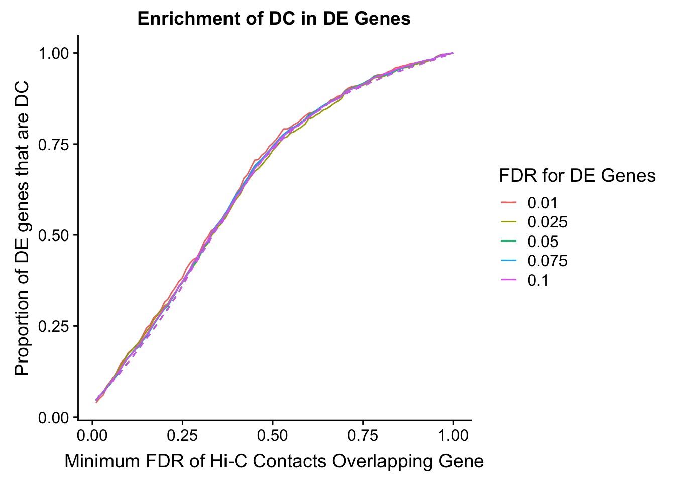
    DEFDR DHICFDR   prop.obs   prop.exp    chisq.p Dneither  DE DHiC Dboth
101 0.025    0.01 0.04602109 0.04598145 1.00000000     6412 995  309    48
102 0.025    0.02 0.05848514 0.05963421 0.92180398     6319 982  402    61
103 0.025    0.03 0.06807287 0.06942298 0.90534608     6253 972  468    71
104 0.025    0.04 0.08533078 0.08037094 0.56728856     6186 954  535    89
105 0.025    0.05 0.09779482 0.09222050 0.54104946     6107 941  614   102
106 0.025    0.06 0.11217641 0.10419887 0.39427305     6029 926  692   117
107 0.025    0.07 0.12751678 0.11424523 0.16276235     5967 910  754   133
108 0.025    0.08 0.14477469 0.12660999 0.06488555     5889 892  832   151
109 0.025    0.09 0.15915628 0.14026275 0.06567647     5798 877  923   166
110 0.025    0.10 0.17449664 0.15108192 0.02621767     5730 861  991   182
111 0.025    0.11 0.18408437 0.16280268 0.05048324     5649 851 1072   192
112 0.025    0.12 0.19558965 0.17709943 0.10149612     5550 839 1171   204
113 0.025    0.13 0.20517737 0.18907779 0.16615517     5467 829 1254   214
114 0.025    0.14 0.22051774 0.20260175 0.13211565     5378 813 1343   230
115 0.025    0.15 0.23489933 0.21586811 0.11753927     5290 798 1431   245
116 0.025    0.16 0.24736337 0.22797527 0.11770441     5209 785 1512   258
117 0.025    0.17 0.26749760 0.24252962 0.04734506     5117 764 1604   279
118 0.025    0.18 0.27996165 0.25540958 0.05535409     5030 751 1691   292
119 0.025    0.19 0.29242570 0.27009274 0.08755444     4929 738 1792   305
120 0.025    0.20 0.30488974 0.28657908 0.17104689     4814 725 1907   318
121 0.025    0.21 0.31255992 0.29752705 0.26916534     4737 717 1984   326
122 0.025    0.22 0.32981783 0.31491499 0.28108959     4620 699 2101   344
123 0.025    0.23 0.34228188 0.32843895 0.32330574     4528 686 2193   357
124 0.025    0.24 0.35858102 0.34453890 0.32185392     4420 669 2301   374
125 0.025    0.25 0.36912752 0.36128284 0.59458342     4301 658 2420   385
126 0.025    0.26 0.38638543 0.37854199 0.59818411     4185 640 2536   403
127 0.025    0.27 0.40076702 0.39657393 0.79215580     4060 625 2661   418
128 0.025    0.28 0.41514861 0.41409067 0.96747895     3939 610 2782   433
129 0.025    0.29 0.42761266 0.42928903 0.93310346     3834 597 2887   446
130 0.025    0.30 0.44774688 0.44448738 0.84601732     3737 576 2984   467
131 0.025    0.31 0.46692234 0.46032973 0.67030073     3634 556 3087   487
132 0.025    0.32 0.47651007 0.47359608 0.86559920     3541 546 3180   497
133 0.025    0.33 0.49760307 0.49330242 0.79077540     3410 524 3311   519
134 0.025    0.34 0.51006711 0.50901597 0.96833309     3301 511 3420   532
135 0.025    0.35 0.52348993 0.52357032 1.00000000     3202 497 3519   546
136 0.025    0.36 0.53307766 0.53464709 0.93953415     3126 487 3595   556
137 0.025    0.37 0.55033557 0.55229263 0.91784465     3007 469 3714   574
138 0.025    0.38 0.56759348 0.57109737 0.83201100     2879 451 3842   592
139 0.025    0.39 0.58581016 0.58861412 0.86975309     2762 432 3959   611
140 0.025    0.40 0.60115053 0.60497166 0.81243992     2651 416 4070   627
141 0.025    0.41 0.61265580 0.61862442 0.69485565     2557 404 4164   639
142 0.025    0.42 0.63374880 0.63369397 1.00000000     2462 382 4259   661
143 0.025    0.43 0.64813039 0.64837713 1.00000000     2363 367 4358   676
144 0.025    0.44 0.66155321 0.66138588 1.00000000     2276 353 4445   690
145 0.025    0.45 0.67497603 0.67928903 0.77557036     2151 339 4570   704
146 0.025    0.46 0.68264621 0.69178259 0.51520095     2062 331 4659   712
147 0.025    0.47 0.69319271 0.70376095 0.44310203     1980 320 4741   723
148 0.025    0.48 0.70565676 0.71470891 0.50990075     1908 307 4813   736
149 0.025    0.49 0.71716203 0.72501288 0.56661085     1840 295 4881   748
150 0.025    0.50 0.73250240 0.73634724 0.79091116     1768 279 4953   764
151 0.025    0.51 0.74304890 0.74510562 0.90002284     1711 268 5010   775
152 0.025    0.52 0.75551294 0.75643998 0.97112240     1636 255 5085   788
153 0.025    0.53 0.76605944 0.76738794 0.94438418     1562 244 5159   799
154 0.025    0.54 0.76989453 0.77460072 0.72549294     1510 240 5211   803
155 0.025    0.55 0.78044104 0.78554869 0.69549200     1436 229 5285   814
156 0.025    0.56 0.78427613 0.79224626 0.52158901     1388 225 5333   818
157 0.025    0.57 0.79098754 0.79894384 0.51727543     1343 218 5378   825
158 0.025    0.58 0.79674017 0.80757342 0.36193260     1282 212 5439   831
159 0.025    0.59 0.80536913 0.81543019 0.39127591     1230 203 5491   840
160 0.025    0.60 0.81975072 0.82290057 0.80815024     1187 188 5534   855
161 0.025    0.61 0.82166826 0.82972694 0.48396946     1136 186 5585   857
162 0.025    0.62 0.82933845 0.83681092 0.51126608     1089 178 5632   865
163 0.025    0.63 0.83413231 0.84312210 0.41664566     1045 173 5676   870
164 0.025    0.64 0.84276127 0.84981968 0.52267074     1002 164 5719   879
165 0.025    0.65 0.84659636 0.85793405 0.28032538      943 160 5778   883
166 0.025    0.66 0.85330777 0.86476043 0.26536782      897 153 5824   890
167 0.025    0.67 0.86097795 0.87107161 0.31933472      856 145 5865   898
168 0.025    0.68 0.86673058 0.87493560 0.41755218      832 139 5889   904
169 0.025    0.69 0.87440077 0.88060278 0.54014141      796 131 5925   912
170 0.025    0.70 0.89165868 0.88730036 0.67026956      762 113 5959   930
171 0.025    0.71 0.89741131 0.89167955 0.55745201      734 107 5987   936
172 0.025    0.72 0.90220518 0.89760433 0.63700890      693 102 6028   941
173 0.025    0.73 0.90508150 0.90069552 0.65025245      672  99 6049   944
174 0.025    0.74 0.90795781 0.90494590 0.76438601      642  96 6079   947
175 0.025    0.75 0.91083413 0.90868109 0.84017248      616  93 6105   950
176 0.025    0.76 0.91658677 0.91228748 0.63926204      594  87 6127   956
177 0.025    0.77 0.92138063 0.91834106 0.74554778      552  82 6169   961
178 0.025    0.78 0.93096836 0.92323545 0.34427129      524  72 6197   971
179 0.025    0.79 0.93288591 0.92658423 0.43842128      500  70 6221   973
180 0.025    0.80 0.93288591 0.93044822 0.78931050      470  70 6251   973
181 0.025    0.81 0.93672100 0.93379701 0.73289298      448  66 6273   977
182 0.025    0.82 0.93959732 0.93766100 0.83431392      421  63 6300   980
183 0.025    0.83 0.94343241 0.94268418 0.96797718      386  59 6335   984
184 0.025    0.84 0.95014382 0.94654817 0.63059228      363  52 6358   991
185 0.025    0.85 0.95493768 0.94938176 0.42149849      346  47 6375   996
186 0.025    0.86 0.95877277 0.95260175 0.35249852      325  43 6396  1000
187 0.025    0.87 0.95973154 0.95646574 0.63551112      296  42 6425  1001
188 0.025    0.88 0.96260786 0.95981453 0.68256049      273  39 6448  1004
189 0.025    0.89 0.96644295 0.96277692 0.55902110      254  35 6467  1008
190 0.025    0.90 0.96931927 0.96586811 0.56994919      233  32 6488  1011
191 0.025    0.91 0.97219559 0.96857290 0.53172936      215  29 6506  1014
192 0.025    0.92 0.97507191 0.97256569 0.66668311      187  26 6534  1017
193 0.025    0.93 0.97794823 0.97617208 0.76788983      162  23 6559  1020
194 0.025    0.94 0.97986577 0.97913447 0.95121777      141  21 6580  1022
195 0.025    0.95 0.98561841 0.98196806 0.40814652      125  15 6596  1028
196 0.025    0.96 0.99232982 0.98596084 0.08227945      101   8 6620  1035
197 0.025    0.97 0.99424736 0.98969603 0.16162088       74   6 6647  1037
198 0.025    0.98 0.99616491 0.99291602 0.25169704       51   4 6670  1039
199 0.025    0.99 0.99712368 0.99639361 0.88458574       25   3 6696  1040
200 0.025    1.00 1.00000000 1.00000000 0.00000000        0   0 6721  1043
enrichment.plotter(gene.hic.filt, "min_FDR.C", "adj.P.Val", "Minimum FDR of Hi-C Contacts Overlapping Gene, Chimp")Warning in chisq.test(mytable): Chi-squared approximation may be incorrect
Warning in chisq.test(mytable): Chi-squared approximation may be incorrect
Warning in chisq.test(mytable): Chi-squared approximation may be incorrect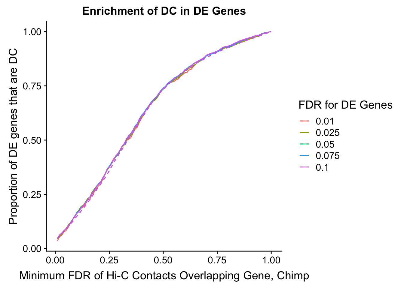
    DEFDR DHICFDR   prop.obs   prop.exp    chisq.p Dneither  DE DHiC Dboth
101 0.025    0.01 0.04339441 0.04602134 0.72328641     6429 992  313    45
102 0.025    0.02 0.05785921 0.06029053 0.77697904     6333 977  409    60
103 0.025    0.03 0.06557377 0.06877491 0.71016249     6275 969  467    68
104 0.025    0.04 0.08100289 0.08073017 1.00000000     6198 953  544    84
105 0.025    0.05 0.09257473 0.09114282 0.90912239     6129 941  613    96
106 0.025    0.06 0.10800386 0.10309808 0.61482727     6052 925  690   112
107 0.025    0.07 0.11957570 0.11261088 0.47810469     5990 913  752   124
108 0.025    0.08 0.13404050 0.12366628 0.29861816     5919 898  823   139
109 0.025    0.09 0.14850530 0.13793547 0.31158300     5823 883  919   154
110 0.025    0.10 0.16682739 0.14924798 0.09697646     5754 864  988   173
111 0.025    0.11 0.17839923 0.15953207 0.08243235     5686 852 1056   185
112 0.025    0.12 0.19479267 0.17380126 0.06118745     5592 835 1150   202
113 0.025    0.13 0.19961427 0.18524232 0.21619429     5508 830 1234   207
114 0.025    0.14 0.21504339 0.19822599 0.15638153     5423 814 1319   223
115 0.025    0.15 0.23047252 0.21262373 0.14205899     5327 798 1415   239
116 0.025    0.16 0.23722276 0.22355058 0.27346858     5249 791 1493   246
117 0.025    0.17 0.25940212 0.24051935 0.13643216     5140 768 1602   269
118 0.025    0.18 0.27290260 0.25388867 0.14079902     5050 754 1692   283
119 0.025    0.19 0.28640309 0.26828641 0.16859407     4952 740 1790   297
120 0.025    0.20 0.29701061 0.28486952 0.37158366     4834 729 1908   308
121 0.025    0.21 0.30568949 0.29605348 0.48793635     4756 720 1986   317
122 0.025    0.22 0.32497589 0.31302224 0.39216772     4644 700 2098   337
123 0.025    0.23 0.34040501 0.32536316 0.28239517     4564 684 2178   353
124 0.025    0.24 0.36065574 0.34156061 0.17458186     4459 663 2283   374
125 0.025    0.25 0.37415622 0.35878648 0.28298069     4339 649 2403   388
126 0.025    0.26 0.39247830 0.37652655 0.26941668     4220 630 2522   407
127 0.025    0.27 0.40597878 0.39400951 0.41612044     4098 616 2644   421
128 0.025    0.28 0.42237223 0.41136393 0.45934370     3980 599 2762   438
129 0.025    0.29 0.43297975 0.42666152 0.68315673     3872 588 2870   449
130 0.025    0.30 0.45033751 0.44375884 0.67123277     3757 570 2985   467
131 0.025    0.31 0.46865959 0.45879933 0.51504613     3659 551 3083   486
132 0.025    0.32 0.47733848 0.47229721 0.75208694     3563 542 3179   495
133 0.025    0.33 0.49951784 0.49157989 0.60594389     3436 519 3306   518
134 0.025    0.34 0.51205400 0.50803445 0.80664861     3321 506 3421   531
135 0.025    0.35 0.52169720 0.52230364 0.99313349     3220 496 3522   541
136 0.025    0.36 0.53519769 0.53451600 0.98896077     3139 482 3603   555
137 0.025    0.37 0.55737705 0.54968505 0.61618466     3044 459 3698   578
138 0.025    0.38 0.56509161 0.56742512 0.89715287     2914 451 3828   586
139 0.025    0.39 0.58919961 0.58645070 0.87350012     2791 426 3951   611
140 0.025    0.40 0.60559306 0.60264816 0.86180029     2682 409 4060   628
141 0.025    0.41 0.61812922 0.61588893 0.90049677     2592 396 4150   641
142 0.025    0.42 0.63934426 0.63092943 0.56960568     2497 374 4245   663
143 0.025    0.43 0.65188042 0.64622702 0.70832401     2391 361 4351   676
144 0.025    0.44 0.66441659 0.65972490 0.75859835     2299 348 4443   689
145 0.025    0.45 0.67695275 0.67630801 0.99041010     2183 335 4559   702
146 0.025    0.46 0.68370299 0.68903458 0.71706379     2091 328 4651   709
147 0.025    0.47 0.69334619 0.70111840 0.58172916     2007 318 4735   719
148 0.025    0.48 0.70973963 0.71294511 0.83504903     1932 301 4810   736
149 0.025    0.49 0.72420444 0.72310066 0.96167390     1868 286 4874   751
150 0.025    0.50 0.73674060 0.73415606 0.86924988     1795 273 4947   764
151 0.025    0.51 0.74445516 0.74238334 0.89994085     1739 265 5003   772
152 0.025    0.52 0.75795564 0.75408150 0.78526707     1662 251 5080   786
153 0.025    0.53 0.76374156 0.76385139 1.00000000     1592 245 5150   792
154 0.025    0.54 0.76759884 0.77143592 0.78226707     1537 241 5205   796
155 0.025    0.55 0.77724204 0.78133436 0.76256334     1470 231 5272   806
156 0.025    0.56 0.78302797 0.78891888 0.64661275     1417 225 5325   812
157 0.025    0.57 0.78784957 0.79637486 0.48963611     1364 220 5378   817
158 0.025    0.58 0.79749277 0.80460213 0.56316613     1310 210 5432   827
159 0.025    0.59 0.80520733 0.81218666 0.56500294     1259 202 5483   835
160 0.025    0.60 0.81870781 0.81951408 0.97674471     1216 188 5526   849
161 0.025    0.61 0.82160077 0.82529888 0.76955046     1174 185 5568   852
162 0.025    0.62 0.83124397 0.83185499 0.99049083     1133 175 5609   862
163 0.025    0.63 0.83413693 0.83879676 0.69433091     1082 172 5660   865
164 0.025    0.64 0.84378014 0.84560998 0.89734367     1039 162 5703   875
165 0.025    0.65 0.85053038 0.85229464 0.90052882      994 155 5748   882
166 0.025    0.66 0.85728062 0.85936496 0.87334096      946 148 5796   889
167 0.025    0.67 0.86306654 0.86502121 0.88150393      908 142 5834   895
168 0.025    0.68 0.87078110 0.86913485 0.90496213      884 134 5858   903
169 0.025    0.69 0.87463838 0.87401980 0.98865360      850 130 5892   907
170 0.025    0.70 0.89006750 0.88031881 0.32339288      817 114 5925   923
171 0.025    0.71 0.89296046 0.88520375 0.42989909      782 111 5960   926
172 0.025    0.72 0.89778206 0.89137421 0.51007701      739 106 6003   931
173 0.025    0.73 0.90067502 0.89535930 0.58490805      711 103 6031   934
174 0.025    0.74 0.90356798 0.89973004 0.69915301      680 100 6062   937
175 0.025    0.75 0.90646095 0.90448644 0.86058638      646  97 6096   940
176 0.025    0.76 0.91128255 0.90847153 0.77996746      620  92 6122   945
177 0.025    0.77 0.91803279 0.91399923 0.66127072      584  85 6158   952
178 0.025    0.78 0.92381871 0.91862707 0.55129117      554  79 6188   958
179 0.025    0.79 0.92574735 0.92248361 0.71898993      526  77 6216   960
180 0.025    0.80 0.92671167 0.92646870 1.00000000      496  76 6246   961
181 0.025    0.81 0.92864031 0.92929682 0.98122857      476  74 6266   963
182 0.025    0.82 0.93346191 0.93366757 1.00000000      447  69 6295   968
183 0.025    0.83 0.93828351 0.93906672 0.96527679      410  64 6332   973
184 0.025    0.84 0.94214079 0.94215195 1.00000000      390  60 6352   977
185 0.025    0.85 0.94792671 0.94575138 0.79596869      368  54 6374   983
186 0.025    0.86 0.95178399 0.95037923 0.88316524      336  50 6406   987
187 0.025    0.87 0.95274831 0.95410721 0.88476661      308  49 6434   988
188 0.025    0.88 0.95756991 0.95834940 0.95894465      280  44 6462   993
189 0.025    0.89 0.96046287 0.96143463 0.92991609      259  41 6483   996
190 0.025    0.90 0.96528447 0.96490551 1.00000000      237  36 6505  1001
191 0.025    0.91 0.96914176 0.96734799 0.79850802      222  32 6520  1005
192 0.025    0.92 0.97396336 0.97159018 0.69379510      194  27 6548  1010
193 0.025    0.93 0.97685632 0.97544672 0.83578036      167  24 6575  1013
194 0.025    0.94 0.97782064 0.97827484 1.00000000      146  23 6596  1014
195 0.025    0.95 0.98457088 0.98213138 0.60929212      123  16 6619  1021
196 0.025    0.96 0.99035680 0.98624502 0.28105941       97  10 6645  1027
197 0.025    0.97 0.99228544 0.99010156 0.55211311       69   8 6673  1029
198 0.025    0.98 0.99421408 0.99305823 0.77896570       48   6 6694  1031
199 0.025    0.99 0.99807136 0.99652912 0.53296052       25   2 6717  1035
200 0.025    1.00 1.00000000 1.00000000 0.00000000        0   0 6742  1037
#enrichment.plotter(h_US, "USFDR", "adj.P.Val", "FDR for Closest Upstream Hi-C Contact Overlapping Gene, Human") #These two are ugly, and can't be run anyway until next chunk is complete to create their DFs. It's OK without them.
#enrichment.plotter(c_US, "USFDR", "adj.P.Val", "FDR for Closest Upstream Hi-C Contact Overlapping Gene, Chimp")
enrichment.plotter(gene.hic.filt, "max_B_FDR.H", "adj.P.Val", "FDR for Hi-C Contact Overlapping Gene w/ Strongest Effect Size, Human")Warning in chisq.test(mytable): Chi-squared approximation may be incorrect
Warning in chisq.test(mytable): Chi-squared approximation may be incorrect
Warning in chisq.test(mytable): Chi-squared approximation may be incorrect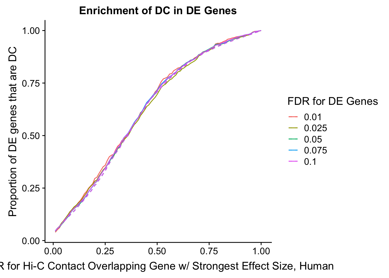
    DEFDR DHICFDR   prop.obs   prop.exp    chisq.p Dneither  DE DHiC Dboth
101 0.025    0.01 0.04410355 0.04482226 0.96797521     6419 997  302    46
102 0.025    0.02 0.05848514 0.05873261 1.00000000     6326 982  395    61
103 0.025    0.03 0.06807287 0.06774858 1.00000000     6266 972  455    71
104 0.025    0.04 0.08341323 0.07792375 0.51648247     6203 956  518    87
105 0.025    0.05 0.09491850 0.08861412 0.47678815     6132 944  589    99
106 0.025    0.06 0.10834132 0.09994848 0.35975878     6058 930  663   113
107 0.025    0.07 0.12176414 0.10935085 0.18439223     5999 916  722   127
108 0.025    0.08 0.13614573 0.12017002 0.09807805     5930 901  791   142
109 0.025    0.09 0.14765101 0.13227718 0.12700571     5848 889  873   154
110 0.025    0.10 0.16011505 0.14013395 0.05116591     5800 876  921   167
111 0.025    0.11 0.16778523 0.15108192 0.11583942     5723 868  998   175
112 0.025    0.12 0.17833174 0.16280268 0.15707440     5643 857 1078   186
113 0.025    0.13 0.18696069 0.17349304 0.23382277     5569 848 1152   195
114 0.025    0.14 0.19942474 0.18495621 0.21106396     5493 835 1228   208
115 0.025    0.15 0.21380633 0.19706337 0.15584384     5414 820 1307   223
116 0.025    0.16 0.22722915 0.20852653 0.11946554     5339 806 1382   237
117 0.025    0.17 0.24640460 0.22230809 0.04865798     5252 786 1469   257
118 0.025    0.18 0.25790988 0.23402885 0.05504120     5173 774 1548   269
119 0.025    0.19 0.26845638 0.24729521 0.09612592     5081 763 1640   280
120 0.025    0.20 0.28283797 0.26313756 0.12973070     4973 748 1748   295
121 0.025    0.21 0.28859060 0.27228233 0.21708427     4908 742 1813   301
122 0.025    0.22 0.30680729 0.28851108 0.17225277     4801 723 1920   320
123 0.025    0.23 0.32118888 0.30203503 0.15801141     4711 708 2010   335
124 0.025    0.24 0.33652924 0.31736218 0.16342653     4608 692 2113   351
125 0.025    0.25 0.34611697 0.33191654 0.31182231     4505 682 2216   361
126 0.025    0.26 0.36241611 0.35097888 0.42548848     4374 665 2347   378
127 0.025    0.27 0.37967402 0.36810922 0.42496919     4259 647 2462   396
128 0.025    0.28 0.39213806 0.38446677 0.60783602     4145 634 2576   409
129 0.025    0.29 0.40076702 0.39966512 0.96481406     4036 625 2685   418
130 0.025    0.30 0.41994247 0.41486347 0.74590232     3938 605 2783   438
131 0.025    0.31 0.43720038 0.42967543 0.62128531     3841 587 2880   456
132 0.025    0.32 0.44487057 0.44165379 0.84825697     3756 579 2965   464
133 0.025    0.33 0.46500479 0.46097372 0.80466066     3627 558 3094   485
134 0.025    0.34 0.47938639 0.47578568 0.82825249     3527 543 3194   500
135 0.025    0.35 0.48993289 0.48969603 1.00000000     3430 532 3291   511
136 0.025    0.36 0.49952061 0.50167439 0.90746178     3347 522 3374   521
137 0.025    0.37 0.51773730 0.52073673 0.86100265     3218 503 3503   540
138 0.025    0.38 0.53691275 0.53941267 0.88810084     3093 483 3628   560
139 0.025    0.39 0.55225312 0.55692942 0.76931887     2973 467 3748   576
140 0.025    0.40 0.56279962 0.57264297 0.51115662     2862 456 3859   587
141 0.025    0.41 0.57526366 0.58629572 0.45702754     2769 443 3952   600
142 0.025    0.42 0.59539789 0.60226687 0.65043398     2666 422 4055   621
143 0.025    0.43 0.60786194 0.61720762 0.52662942     2563 409 4158   634
144 0.025    0.44 0.62224353 0.63008758 0.59645414     2478 394 4243   649
145 0.025    0.45 0.63854267 0.64799073 0.51451041     2356 377 4365   666
146 0.025    0.46 0.64621285 0.66164348 0.27270818     2258 369 4463   674
147 0.025    0.47 0.65963567 0.67555384 0.25234643     2164 355 4557   688
148 0.025    0.48 0.67114094 0.68650180 0.26550979     2091 343 4630   700
149 0.025    0.49 0.68168744 0.69577537 0.30455679     2030 332 4691   711
150 0.025    0.50 0.69606903 0.70852653 0.36023834     1946 317 4775   726
151 0.025    0.51 0.71332694 0.71818650 0.73539655     1889 299 4832   744
152 0.025    0.52 0.72962608 0.73042246 0.98021707     1811 282 4910   761
153 0.025    0.53 0.73921381 0.74227202 0.83783935     1729 272 4992   771
154 0.025    0.54 0.74496644 0.75128800 0.63897896     1665 266 5056   777
155 0.025    0.55 0.75551294 0.76339516 0.54543469     1582 255 5139   788
156 0.025    0.56 0.76510067 0.77241113 0.57171214     1522 245 5199   798
157 0.025    0.57 0.76989453 0.77988150 0.42573110     1469 240 5252   803
158 0.025    0.58 0.78044104 0.78967027 0.45612742     1404 229 5317   814
159 0.025    0.59 0.78811122 0.79778465 0.42687172     1349 221 5372   822
160 0.025    0.60 0.80345158 0.80654302 0.81845530     1297 205 5424   838
161 0.025    0.61 0.80632790 0.81465739 0.48315154     1237 202 5484   841
162 0.025    0.62 0.81783317 0.82264297 0.69393543     1187 190 5534   853
163 0.025    0.63 0.82262704 0.82934055 0.56516250     1140 185 5581   858
164 0.025    0.64 0.83125599 0.83719732 0.60757686     1088 176 5633   867
165 0.025    0.65 0.83604986 0.84621329 0.35143663     1023 171 5698   872
166 0.025    0.66 0.84372004 0.85394127 0.33832325      971 163 5750   880
167 0.025    0.67 0.84947267 0.86038125 0.29626238      927 157 5794   886
168 0.025    0.68 0.85522531 0.86450283 0.37223280      901 151 5820   892
169 0.025    0.69 0.86385427 0.87107161 0.48523775      859 142 5862   901
170 0.025    0.70 0.87919463 0.87815559 0.95264298      820 126 5901   917
171 0.025    0.71 0.88398849 0.88330757 0.98261612      785 121 5936   922
172 0.025    0.72 0.89357622 0.89116435 0.82946532      734 111 5987   932
173 0.025    0.73 0.89837009 0.89528594 0.76777009      707 106 6014   937
174 0.025    0.74 0.90124640 0.90043792 0.96956620      670 103 6051   940
175 0.025    0.75 0.90604027 0.90443071 0.89384996      644  98 6077   945
176 0.025    0.76 0.91179291 0.90803709 0.69390656      622  92 6099   951
177 0.025    0.77 0.91658677 0.91447707 0.83964058      577  87 6144   956
178 0.025    0.78 0.93000959 0.92014426 0.22940588      547  73 6174   970
179 0.025    0.79 0.93192713 0.92387944 0.32187030      520  71 6201   972
180 0.025    0.80 0.93192713 0.92787223 0.63140801      489  71 6232   972
181 0.025    0.81 0.93576222 0.93134982 0.58926313      466  67 6255   976
182 0.025    0.82 0.93863854 0.93572901 0.73087002      435  64 6286   979
183 0.025    0.83 0.94247363 0.94062339 0.84042744      401  60 6320   983
184 0.025    0.84 0.94822627 0.94474498 0.64834678      375  54 6346   989
185 0.025    0.85 0.95302013 0.94757857 0.43962883      358  49 6363   994
186 0.025    0.86 0.95781400 0.95105616 0.31244262      336  44 6385   999
187 0.025    0.87 0.95877277 0.95492014 0.57252310      307  43 6414  1000
188 0.025    0.88 0.96260786 0.95878413 0.55924440      281  39 6440  1004
189 0.025    0.89 0.96644295 0.96251932 0.52906158      256  35 6465  1008
190 0.025    0.90 0.96836050 0.96548171 0.64823182      235  33 6486  1010
191 0.025    0.91 0.97123682 0.96805770 0.59409550      218  30 6503  1013
192 0.025    0.92 0.97507191 0.97217929 0.61051223      190  26 6531  1017
193 0.025    0.93 0.97698945 0.97591448 0.89273525      163  24 6558  1019
194 0.025    0.94 0.97890700 0.97887687 1.00000000      142  22 6579  1021
195 0.025    0.95 0.98465964 0.98183926 0.54283717      125  16 6596  1027
196 0.025    0.96 0.99232982 0.98596084 0.08227945      101   8 6620  1035
197 0.025    0.97 0.99424736 0.98969603 0.16162088       74   6 6647  1037
198 0.025    0.98 0.99616491 0.99291602 0.25169704       51   4 6670  1039
199 0.025    0.99 0.99712368 0.99639361 0.88458574       25   3 6696  1040
200 0.025    1.00 1.00000000 1.00000000 0.00000000        0   0 6721  1043
enrichment.plotter(gene.hic.filt, "max_B_FDR.C", "adj.P.Val", "FDR for Hi-C Contact Overlapping Gene w/ Strongest Effect Size, Chimp")Warning in chisq.test(mytable): Chi-squared approximation may be incorrect
Warning in chisq.test(mytable): Chi-squared approximation may be incorrect
Warning in chisq.test(mytable): Chi-squared approximation may be incorrect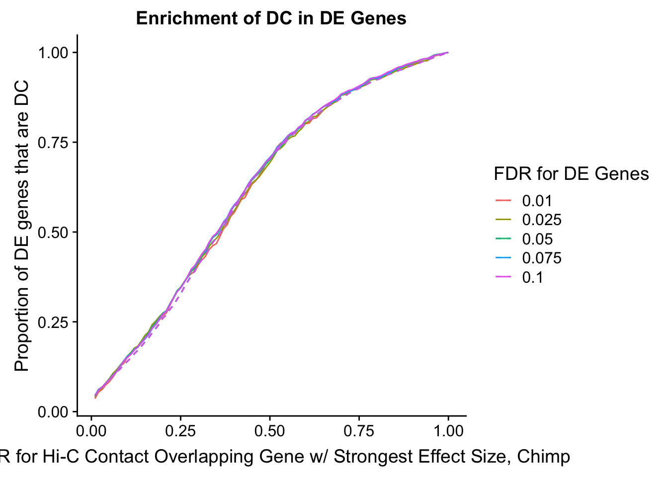
    DEFDR DHICFDR   prop.obs   prop.exp    chisq.p Dneither  DE DHiC Dboth
101 0.025    0.01 0.04050145 0.04422162 0.58588865     6440 995  302    42
102 0.025    0.02 0.05785921 0.05913356 0.90751480     6342 977  400    60
103 0.025    0.03 0.06557377 0.06710374 0.88482114     6288 969  454    68
104 0.025    0.04 0.08003857 0.07828770 0.87022587     6216 954  526    83
105 0.025    0.05 0.09161041 0.08792904 0.69596818     6153 942  589    95
106 0.025    0.06 0.10607522 0.09949865 0.48126631     6078 927  664   110
107 0.025    0.07 0.11571842 0.10824013 0.43602319     6020 917  722   120
108 0.025    0.08 0.12825458 0.11813858 0.30187099     5956 904  786   133
109 0.025    0.09 0.13886210 0.13022239 0.40178621     5873 893  869   144
110 0.025    0.10 0.15332690 0.13909243 0.16922958     5819 878  923   159
111 0.025    0.11 0.16393443 0.14899087 0.16007538     5753 867  989   170
112 0.025    0.12 0.17647059 0.16068903 0.14957291     5675 854 1067   183
113 0.025    0.13 0.18225651 0.17058748 0.30360077     5604 848 1138   189
114 0.025    0.14 0.19672131 0.18151433 0.18635635     5534 833 1208   204
115 0.025    0.15 0.21215043 0.19449801 0.13347864     5449 817 1293   220
116 0.025    0.16 0.22179364 0.20439645 0.14680121     5382 807 1360   230
117 0.025    0.17 0.24204436 0.21943695 0.06442748     5286 786 1456   251
118 0.025    0.18 0.25168756 0.23113511 0.09958999     5205 776 1537   261
119 0.025    0.19 0.26422372 0.24424733 0.11653410     5116 763 1626   274
120 0.025    0.20 0.27386692 0.26005913 0.29336155     5003 753 1739   284
121 0.025    0.21 0.27965284 0.26905772 0.43022442     4939 747 1803   290
122 0.025    0.22 0.29990357 0.28474097 0.26049382     4838 726 1904   311
123 0.025    0.23 0.31629701 0.29708189 0.15619392     4759 709 1983   328
124 0.025    0.24 0.33461909 0.31263659 0.10864494     4657 690 2085   347
125 0.025    0.25 0.34619094 0.32754853 0.18074156     4553 678 2189   359
126 0.025    0.26 0.36162006 0.34657411 0.28977852     4421 662 2321   375
127 0.025    0.27 0.37512054 0.36264301 0.38810623     4310 648 2432   389
128 0.025    0.28 0.39054966 0.37871192 0.41806836     4201 632 2541   405
129 0.025    0.29 0.39922854 0.39375241 0.72366660     4093 623 2649   414
130 0.025    0.30 0.41562199 0.41046407 0.74231587     3980 606 2762   431
131 0.025    0.31 0.43105111 0.42434760 0.66326352     3888 590 2854   447
132 0.025    0.32 0.44165863 0.43733128 0.78860016     3798 579 2944   458
133 0.025    0.33 0.45998071 0.45532845 0.77208369     3677 560 3065   477
134 0.025    0.34 0.47348120 0.47062604 0.86937694     3572 546 3170   491
135 0.025    0.35 0.48216008 0.48412392 0.91831516     3476 537 3266   500
136 0.025    0.36 0.49469624 0.49697905 0.90086173     3389 524 3353   513
137 0.025    0.37 0.51591128 0.51394781 0.91834496     3279 502 3463   535
138 0.025    0.38 0.52555448 0.53194498 0.68211302     3149 492 3593   545
139 0.025    0.39 0.54773385 0.55084201 0.85509928     3025 469 3717   568
140 0.025    0.40 0.55930569 0.56588250 0.67058671     2920 457 3822   580
141 0.025    0.41 0.57377049 0.58015169 0.67927824     2824 442 3918   595
142 0.025    0.42 0.59402122 0.59634915 0.89646267     2719 421 4023   616
143 0.025    0.43 0.60559306 0.61164674 0.69252726     2612 409 4130   628
144 0.025    0.44 0.62005786 0.62630158 0.68037591     2513 394 4229   643
145 0.025    0.45 0.63645130 0.64378455 0.62069306     2394 377 4348   660
146 0.025    0.46 0.64416586 0.65702532 0.36710736     2299 369 4443   668
147 0.025    0.47 0.65380906 0.67026610 0.23983117     2206 359 4536   678
148 0.025    0.48 0.66730955 0.68222137 0.28372763     2127 345 4615   692
149 0.025    0.49 0.68081003 0.69070575 0.48112428     2075 331 4667   706
150 0.025    0.50 0.69334619 0.70407507 0.43745365     1984 318 4758   719
151 0.025    0.51 0.70877531 0.71358786 0.74039302     1926 302 4816   735
152 0.025    0.52 0.72613308 0.72695719 0.97881899     1840 284 4902   753
153 0.025    0.53 0.73288332 0.73736984 0.75294610     1766 277 4976   760
154 0.025    0.54 0.74252652 0.74701118 0.75012509     1701 267 5041   770
155 0.025    0.55 0.75699132 0.75870935 0.92041380     1625 252 5117   785
156 0.025    0.56 0.76470588 0.76809359 0.81177745     1560 244 5182   793
157 0.025    0.57 0.76759884 0.77657797 0.48043032     1497 241 5245   796
158 0.025    0.58 0.78013500 0.78621931 0.63645097     1435 228 5307   809
159 0.025    0.59 0.78881389 0.79431804 0.66736204     1381 219 5361   818
160 0.025    0.60 0.80327869 0.80331662 1.00000000     1326 204 5416   833
161 0.025    0.61 0.80810029 0.81090114 0.83771287     1272 199 5470   838
162 0.025    0.62 0.82063645 0.81822856 0.86286875     1228 186 5514   851
163 0.025    0.63 0.82256509 0.82568454 0.80997545     1172 184 5570   853
164 0.025    0.64 0.83124397 0.83404037 0.82963969     1116 175 5626   862
165 0.025    0.65 0.83992285 0.84188199 0.88863812     1064 166 5678   871
166 0.025    0.66 0.84763742 0.84985217 0.86676202     1010 158 5732   879
167 0.025    0.67 0.85342334 0.85576552 0.85469454      970 152 5772   885
168 0.025    0.68 0.86017358 0.86013626 1.00000000      943 145 5799   892
169 0.025    0.69 0.86499518 0.86592107 0.96407055      903 140 5839   897
170 0.025    0.70 0.88138862 0.87273428 0.39632701      867 123 5875   914
171 0.025    0.71 0.88331726 0.87787633 0.60037691      829 121 5913   916
172 0.025    0.72 0.89006750 0.88546086 0.65416282      777 114 5965   923
173 0.025    0.73 0.89392478 0.88996015 0.70028750      746 110 5996   927
174 0.025    0.74 0.89681774 0.89535930 0.91214970      707 107 6035   930
175 0.025    0.75 0.90163934 0.90037280 0.92781737      673 102 6069   935
176 0.025    0.76 0.90646095 0.90461499 0.87241173      645  97 6097   940
177 0.025    0.77 0.91224687 0.91027124 0.85655670      607  91 6135   946
178 0.025    0.78 0.92285439 0.91567039 0.40414591      576  80 6166   957
179 0.025    0.79 0.92478303 0.92016969 0.59802288      543  78 6199   959
180 0.025    0.80 0.92574735 0.92428333 0.89784562      512  77 6230   960
181 0.025    0.81 0.92767599 0.92736856 1.00000000      490  75 6252   962
182 0.025    0.82 0.93249759 0.93238205 1.00000000      456  70 6286   967
183 0.025    0.83 0.93731919 0.93778121 1.00000000      419  65 6323   972
184 0.025    0.84 0.94117647 0.94099499 1.00000000      398  61 6344   976
185 0.025    0.85 0.94696239 0.94433732 0.74646237      378  55 6364   982
186 0.025    0.86 0.95081967 0.94935082 0.87631133      343  51 6399   986
187 0.025    0.87 0.95178399 0.95269315 0.94453337      318  50 6424   987
188 0.025    0.88 0.95756991 0.95732099 1.00000000      288  44 6454   993
189 0.025    0.89 0.96046287 0.96117753 0.96679200      261  41 6481   996
190 0.025    0.90 0.96432015 0.96451986 1.00000000      239  37 6503  1000
191 0.025    0.91 0.96817743 0.96696233 0.88720191      224  33 6518  1004
192 0.025    0.92 0.97396336 0.97120453 0.63770366      197  27 6545  1010
193 0.025    0.93 0.97685632 0.97531816 0.81387761      168  24 6574  1013
194 0.025    0.94 0.97782064 0.97814629 1.00000000      147  23 6595  1014
195 0.025    0.95 0.98457088 0.98213138 0.60929212      123  16 6619  1021
196 0.025    0.96 0.99035680 0.98624502 0.28105941       97  10 6645  1027
197 0.025    0.97 0.99228544 0.99010156 0.55211311       69   8 6673  1029
198 0.025    0.98 0.99421408 0.99305823 0.77896570       48   6 6694  1031
199 0.025    0.99 0.99807136 0.99652912 0.53296052       25   2 6717  1035
200 0.025    1.00 1.00000000 1.00000000 0.00000000        0   0 6742  1037
enrichment.plotter(gene.hic.filt, "median_FDR.H", "adj.P.Val", "Median FDR of Hi-C Contacts Overlapping Gene, Human")Warning in chisq.test(mytable): Chi-squared approximation may be incorrect
Warning in chisq.test(mytable): Chi-squared approximation may be incorrect
Warning in chisq.test(mytable): Chi-squared approximation may be incorrect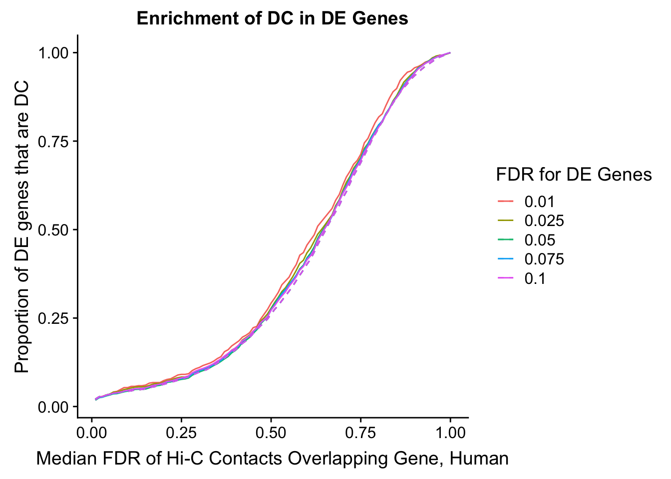
    DEFDR DHICFDR   prop.obs   prop.exp    chisq.p Dneither   DE DHiC
101 0.025    0.01 0.02013423 0.02099433 0.92655649     6579 1022  142
102 0.025    0.02 0.02588686 0.02743431 0.82045151     6535 1016  186
103 0.025    0.03 0.02876318 0.02910871 1.00000000     6525 1013  196
104 0.025    0.04 0.03259827 0.03232870 1.00000000     6504 1009  217
105 0.025    0.05 0.03547459 0.03464709 0.94732058     6489 1006  232
106 0.025    0.06 0.04026846 0.03735188 0.65549902     6473 1001  248
107 0.025    0.07 0.04122723 0.03915507 0.77561650     6460 1000  261
108 0.025    0.08 0.04410355 0.04070067 0.60755904     6451  997  270
109 0.025    0.09 0.04793864 0.04211747 0.35593456     6444  993  277
110 0.025    0.10 0.04985618 0.04314786 0.28728637     6438  991  283
111 0.025    0.11 0.05273250 0.04456466 0.19589493     6430  988  291
112 0.025    0.12 0.05465005 0.04662545 0.21415801     6416  986  305
113 0.025    0.13 0.05560882 0.04752705 0.21487034     6410  985  311
114 0.025    0.14 0.05560882 0.04829985 0.26885388     6404  985  317
115 0.025    0.15 0.05656759 0.05010304 0.34094463     6391  984  330
116 0.025    0.16 0.05944391 0.05280783 0.33930638     6373  981  348
117 0.025    0.17 0.06327900 0.05577022 0.28765695     6354  977  367
118 0.025    0.18 0.06519655 0.05692942 0.24335327     6347  975  374
119 0.025    0.19 0.06519655 0.05989181 0.48026922     6324  975  397
120 0.025    0.20 0.06903164 0.06272540 0.40419343     6306  971  415
121 0.025    0.21 0.07286673 0.06555899 0.33825584     6288  967  433
122 0.025    0.22 0.07478428 0.06890778 0.45954080     6264  965  457
123 0.025    0.23 0.07861937 0.07122617 0.35078791     6250  961  471
124 0.025    0.24 0.08149569 0.07444616 0.38495587     6228  958  493
125 0.025    0.25 0.08341323 0.07766615 0.49449973     6205  956  516
126 0.025    0.26 0.08341323 0.08088614 0.79433669     6180  956  541
127 0.025    0.27 0.08533078 0.08397733 0.91289378     6158  954  563
128 0.025    0.28 0.09300096 0.08925811 0.69114225     6125  946  596
129 0.025    0.29 0.09971237 0.09312210 0.46544355     6102  939  619
130 0.025    0.30 0.10354746 0.09763009 0.52481008     6071  935  650
131 0.025    0.31 0.10642378 0.10110768 0.57759985     6047  932  674
132 0.025    0.32 0.10930010 0.10432767 0.60991646     6025  929  696
133 0.025    0.33 0.11409396 0.11038125 0.72022923     5983  924  738
134 0.025    0.34 0.11984660 0.11591963 0.70854110     5946  918  775
135 0.025    0.35 0.12464046 0.12313241 0.91346815     5895  913  826
136 0.025    0.36 0.13039310 0.12995878 1.00000000     5848  907  873
137 0.025    0.37 0.14093960 0.13691396 0.72027961     5805  896  916
138 0.025    0.38 0.14765101 0.14502834 0.83267369     5749  889  972
139 0.025    0.39 0.15915628 0.15262751 0.55929943     5702  877 1019
140 0.025    0.40 0.16490892 0.15984029 0.66378368     5652  871 1069
141 0.025    0.41 0.17353787 0.16834106 0.66165589     5595  862 1126
142 0.025    0.42 0.18791946 0.17851623 0.41858665     5531  847 1190
143 0.025    0.43 0.19463087 0.18572901 0.45219080     5482  840 1239
144 0.025    0.44 0.20230105 0.19448738 0.52009610     5422  832 1299
145 0.025    0.45 0.21284756 0.20672334 0.62849152     5338  821 1383
146 0.025    0.46 0.22243528 0.21612571 0.62295233     5275  811 1446
147 0.025    0.47 0.24065197 0.22784647 0.30770530     5203  792 1518
148 0.025    0.48 0.25023969 0.23647604 0.27784331     5146  782 1575
149 0.025    0.49 0.26174497 0.24742401 0.26553000     5073  770 1648
150 0.025    0.50 0.27804410 0.26146316 0.20341754     4981  753 1740
151 0.025    0.51 0.29434324 0.27472952 0.13677284     4895  736 1826
152 0.025    0.52 0.30872483 0.28619268 0.09034106     4821  721 1900
153 0.025    0.53 0.32502397 0.29933024 0.05599162     4736  704 1985
154 0.025    0.54 0.33557047 0.31259660 0.09210379     4644  693 2077
155 0.025    0.55 0.35091083 0.32599176 0.07032863     4556  677 2165
156 0.025    0.56 0.36625120 0.33977331 0.05673441     4465  661 2256
157 0.025    0.57 0.38446788 0.35561566 0.03965277     4361  642 2360
158 0.025    0.58 0.40460211 0.37107161 0.01755911     4262  621 2459
159 0.025    0.59 0.41323106 0.38588357 0.05538974     4156  612 2565
160 0.025    0.60 0.43432407 0.40211231 0.02467845     4052  590 2669
161 0.025    0.61 0.44774688 0.41666667 0.03120024     3953  576 2768
162 0.025    0.62 0.46692234 0.43611540 0.03377046     3822  556 2899
163 0.025    0.63 0.48705657 0.45749614 0.04274404     3677  535 3044
164 0.025    0.64 0.49952061 0.47707367 0.12685051     3538  522 3183
165 0.025    0.65 0.51294343 0.49497682 0.22472401     3413  508 3308
166 0.025    0.66 0.52732502 0.51481195 0.40328379     3274  493 3447
167 0.025    0.67 0.54170662 0.53310149 0.57183835     3147  478 3574
168 0.025    0.68 0.56759348 0.55074704 0.25339840     3037  451 3684
169 0.025    0.69 0.58389262 0.56826378 0.28839546     2918  434 3803
170 0.025    0.70 0.61073826 0.58990211 0.15082515     2778  406 3943
171 0.025    0.71 0.63374880 0.60754766 0.06748084     2665  382 4056
172 0.025    0.72 0.65004794 0.63060278 0.17256823     2503  365 4218
173 0.025    0.73 0.67305849 0.65236991 0.14074334     2358  341 4363
174 0.025    0.74 0.68744008 0.67014426 0.21441160     2235  326 4486
175 0.025    0.75 0.70373921 0.68920659 0.29189070     2104  309 4617
176 0.025    0.76 0.72962608 0.70955693 0.13416802     1973  282 4748
177 0.025    0.77 0.74304890 0.72964967 0.31262534     1831  268 4890
178 0.025    0.78 0.76318313 0.75115920 0.35399504     1685  247 5036
179 0.025    0.79 0.78044104 0.76944874 0.38627201     1561  229 5160
180 0.025    0.80 0.79578140 0.78696548 0.47973730     1441  213 5280
181 0.025    0.81 0.80441035 0.80667182 0.87552975     1297  204 5424
182 0.025    0.82 0.82646213 0.82457496 0.89776758     1181  181 5540
183 0.025    0.83 0.84276127 0.84067491 0.87886192     1073  164 5648
184 0.025    0.84 0.86385427 0.85806285 0.59725740      960  142 5761
185 0.025    0.85 0.87823586 0.87287481 0.61097697      860  127 5861
186 0.025    0.86 0.89741131 0.88794436 0.32265851      763  107 5958
187 0.025    0.87 0.91658677 0.90056672 0.07144170      685   87 6036
188 0.025    0.88 0.92713327 0.91228748 0.07792306      605   76 6116
189 0.025    0.89 0.93767977 0.92490984 0.10548658      518   65 6203
190 0.025    0.90 0.94630872 0.93495621 0.12590115      449   56 6272
191 0.025    0.91 0.95781400 0.94345698 0.03701412      395   44 6326
192 0.025    0.92 0.96452541 0.95337455 0.07893351      325   37 6396
193 0.025    0.93 0.97027804 0.96161772 0.13938057      267   31 6454
194 0.025    0.94 0.97698945 0.96831530 0.10438754      222   24 6499
195 0.025    0.95 0.98465964 0.97514168 0.04389353      177   16 6544
196 0.025    0.96 0.99041227 0.98261206 0.05188634      125   10 6596
197 0.025    0.97 0.99232982 0.98737764 0.16431524       90    8 6631
198 0.025    0.98 0.99328859 0.99149923 0.62039809       59    7 6662
199 0.025    0.99 0.99616491 0.99600721 1.00000000       27    4 6694
200 0.025    1.00 1.00000000 1.00000000 0.00000000        0    0 6721
    Dboth
101    21
102    27
103    30
104    34
105    37
106    42
107    43
108    46
109    50
110    52
111    55
112    57
113    58
114    58
115    59
116    62
117    66
118    68
119    68
120    72
121    76
122    78
123    82
124    85
125    87
126    87
127    89
128    97
129   104
130   108
131   111
132   114
133   119
134   125
135   130
136   136
137   147
138   154
139   166
140   172
141   181
142   196
143   203
144   211
145   222
146   232
147   251
148   261
149   273
150   290
151   307
152   322
153   339
154   350
155   366
156   382
157   401
158   422
159   431
160   453
161   467
162   487
163   508
164   521
165   535
166   550
167   565
168   592
169   609
170   637
171   661
172   678
173   702
174   717
175   734
176   761
177   775
178   796
179   814
180   830
181   839
182   862
183   879
184   901
185   916
186   936
187   956
188   967
189   978
190   987
191   999
192  1006
193  1012
194  1019
195  1027
196  1033
197  1035
198  1036
199  1039
200  1043
enrichment.plotter(gene.hic.filt, "median_FDR.C", "adj.P.Val", "Median FDR of Hi-C Contacts Overlapping Gene, Chimp")Warning in chisq.test(mytable): Chi-squared approximation may be incorrect
Warning in chisq.test(mytable): Chi-squared approximation may be incorrect
Warning in chisq.test(mytable): Chi-squared approximation may be incorrect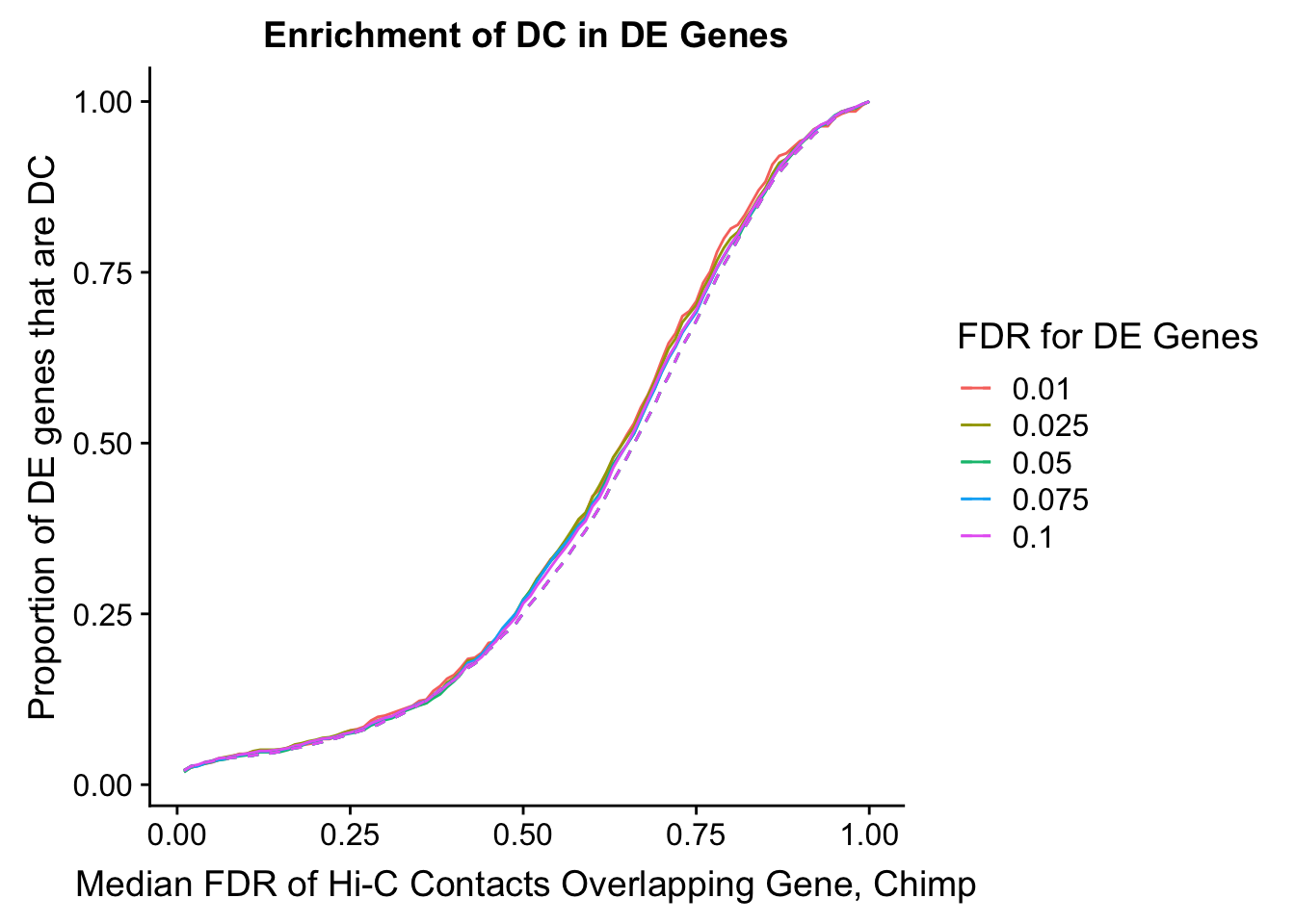
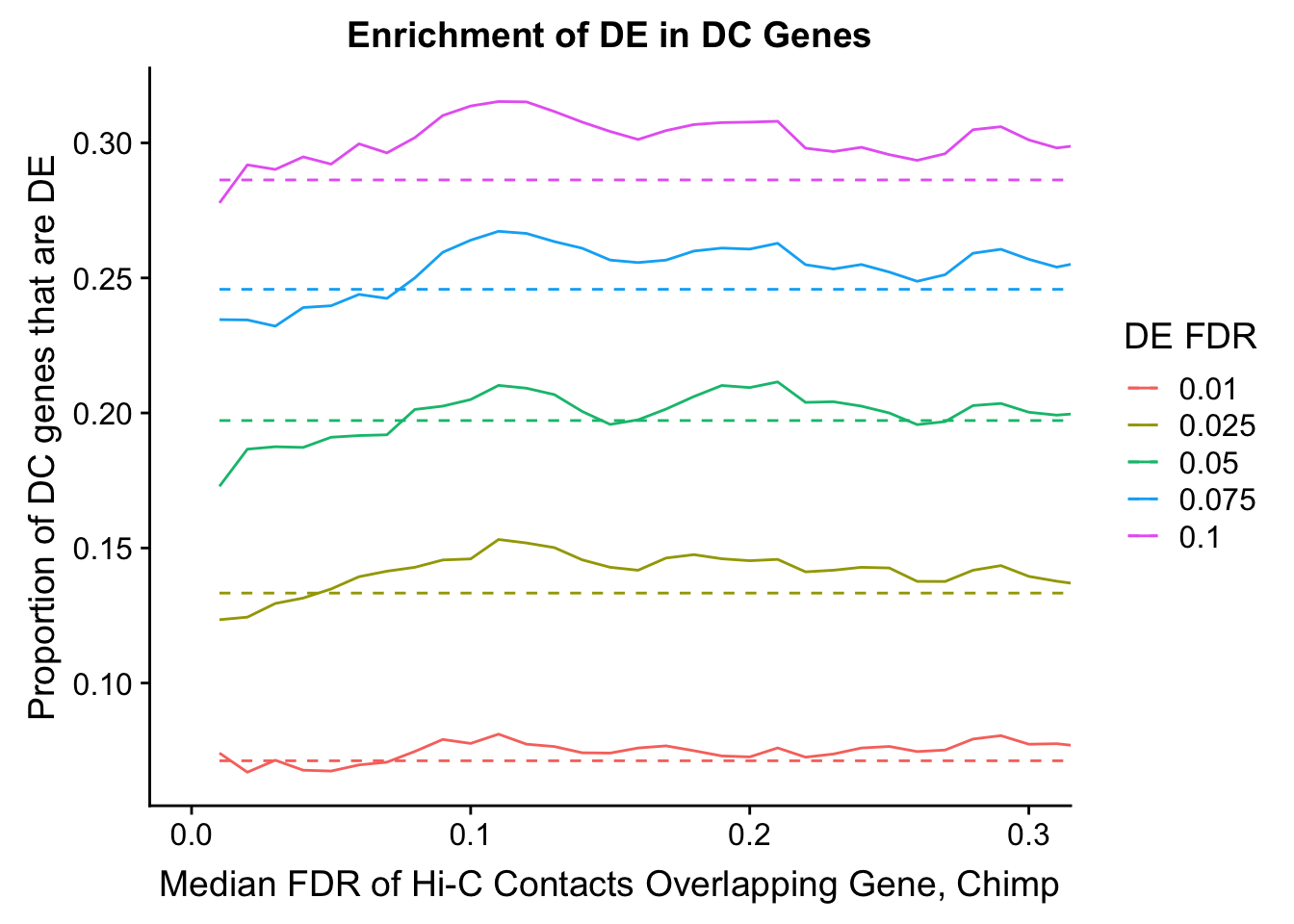
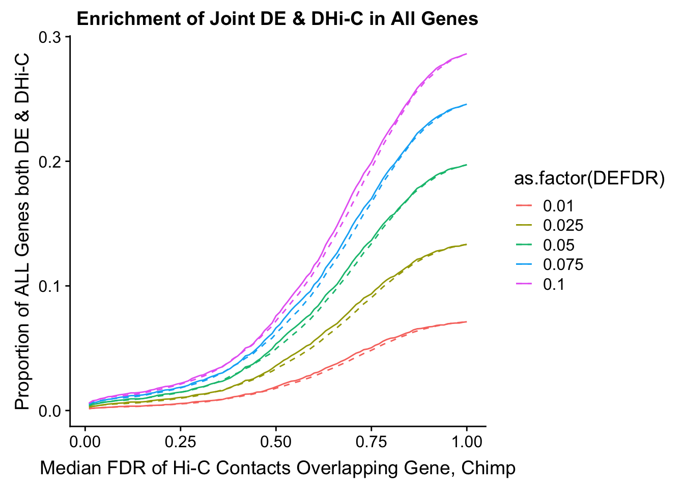
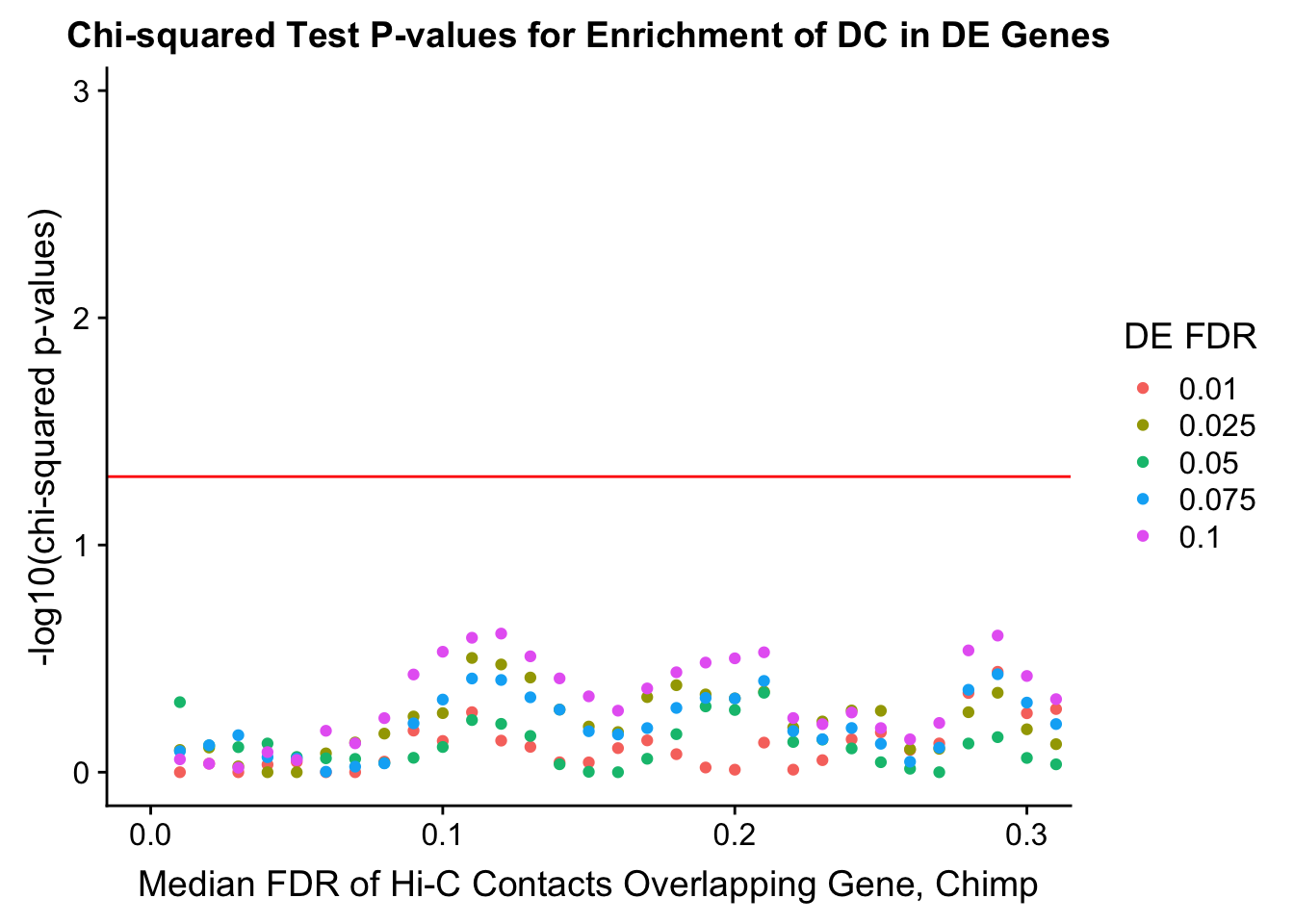
    DEFDR DHICFDR   prop.obs   prop.exp     chisq.p Dneither   DE DHiC
101 0.025    0.01 0.01928640 0.02082530 0.797970136     6600 1017  142
102 0.025    0.02 0.02507232 0.02686721 0.778846246     6559 1011  183
103 0.025    0.03 0.02796528 0.02879547 0.942611913     6547 1008  195
104 0.025    0.04 0.03182257 0.03226636 1.000000000     6524 1004  218
105 0.025    0.05 0.03471553 0.03432318 1.000000000     6511 1001  231
106 0.025    0.06 0.03857281 0.03689420 0.826221764     6495  997  247
107 0.025    0.07 0.04050145 0.03817971 0.739847555     6487  995  255
108 0.025    0.08 0.04243009 0.03959378 0.676247109     6478  993  264
109 0.025    0.09 0.04435873 0.04062219 0.568523068     6472  991  270
110 0.025    0.10 0.04532305 0.04139350 0.549417045     6467  990  275
111 0.025    0.11 0.04918033 0.04280756 0.314126703     6460  986  282
112 0.025    0.12 0.05110897 0.04486438 0.335599946     6446  984  296
113 0.025    0.13 0.05110897 0.04537858 0.383085940     6442  984  300
114 0.025    0.14 0.05110897 0.04679265 0.530018036     6431  984  311
115 0.025    0.15 0.05207329 0.04859236 0.629502431     6418  983  324
116 0.025    0.16 0.05400193 0.05077773 0.665723121     6403  981  339
117 0.025    0.17 0.05882353 0.05360586 0.467075368     6386  976  356
118 0.025    0.18 0.06075217 0.05489137 0.414020852     6378  974  364
119 0.025    0.19 0.06364513 0.05810515 0.454553955     6356  971  386
120 0.025    0.20 0.06557377 0.06016197 0.473307851     6342  969  400
121 0.025    0.21 0.06846673 0.06260445 0.442357075     6326  966  416
122 0.025    0.22 0.06943105 0.06556113 0.635894198     6304  965  438
123 0.025    0.23 0.07232401 0.06800360 0.597935076     6288  962  454
124 0.025    0.24 0.07618129 0.07108883 0.534875220     6268  958  474
125 0.025    0.25 0.07907425 0.07391696 0.536513687     6249  955  493
126 0.025    0.26 0.08003857 0.07751639 0.791868051     6222  954  520
127 0.025    0.27 0.08293153 0.08034452 0.788816252     6203  951  539
128 0.025    0.28 0.08968177 0.08432961 0.544371671     6179  944  563
129 0.025    0.29 0.09450338 0.08780049 0.447054748     6157  939  585
130 0.025    0.30 0.09739634 0.09307109 0.647272374     6119  936  623
131 0.025    0.31 0.09932498 0.09615632 0.752597931     6097  934  645
132 0.025    0.32 0.10318226 0.10091271 0.837370379     6064  930  678
133 0.025    0.33 0.10896818 0.10618331 0.795983400     6029  924  713
134 0.025    0.34 0.11282546 0.11158247 0.933384713     5991  920  751
135 0.025    0.35 0.11668274 0.11801003 0.927800480     5945  916  797
136 0.025    0.36 0.11957570 0.12379483 0.694700141     5903  913  839
137 0.025    0.37 0.13018322 0.13086515 0.983652974     5859  902  883
138 0.025    0.38 0.13693346 0.13934953 0.846830347     5800  895  942
139 0.025    0.39 0.14946962 0.14680550 0.831124383     5755  882  987
140 0.025    0.40 0.15621986 0.15323306 0.809930128     5712  875 1030
141 0.025    0.41 0.16586307 0.16171744 0.730717294     5656  865 1086
142 0.025    0.42 0.18129219 0.17084458 0.359733668     5601  849 1141
143 0.025    0.43 0.18322083 0.17714359 0.612211918     5554  847 1188
144 0.025    0.44 0.18997107 0.18549942 0.722571949     5496  840 1246
145 0.025    0.45 0.20250723 0.19732613 0.682973826     5417  827 1325
146 0.025    0.46 0.21311475 0.20606762 0.574506386     5360  816 1382
147 0.025    0.47 0.22661524 0.21827998 0.510792104     5279  802 1463
148 0.025    0.48 0.23722276 0.22663581 0.403781437     5225  791 1517
149 0.025    0.49 0.25265188 0.23679136 0.210824127     5162  775 1580
150 0.025    0.50 0.27000964 0.25118910 0.143571408     5068  757 1674
151 0.025    0.51 0.28447445 0.26442988 0.124954421     4980  742 1762
152 0.025    0.52 0.30183221 0.27612804 0.051007253     4907  724 1835
153 0.025    0.53 0.31340405 0.28936881 0.072395763     4816  712 1926
154 0.025    0.54 0.32979749 0.30273814 0.045398665     4729  695 2013
155 0.025    0.55 0.34233365 0.31572182 0.051827427     4641  682 2101
156 0.025    0.56 0.35679846 0.32767708 0.034806659     4563  667 2179
157 0.025    0.57 0.37222758 0.34323178 0.037769227     4458  651 2284
158 0.025    0.58 0.38862102 0.35801517 0.029745580     4360  634 2382
159 0.025    0.59 0.39826422 0.37189870 0.063958841     4262  624 2480
160 0.025    0.60 0.42044359 0.38925312 0.029365639     4150  601 2592
161 0.025    0.61 0.43780135 0.40532202 0.024172176     4043  583 2699
162 0.025    0.62 0.45708775 0.42383340 0.021791292     3919  563 2823
163 0.025    0.63 0.47926712 0.44453015 0.017102275     3781  540 2961
164 0.025    0.64 0.49373192 0.46227021 0.031608716     3658  525 3084
165 0.025    0.65 0.50916104 0.47923898 0.041505924     3542  509 3200
166 0.025    0.66 0.52362584 0.49903587 0.095354196     3403  494 3339
167 0.025    0.67 0.54676953 0.51831855 0.052841878     3277  470 3465
168 0.025    0.68 0.56894889 0.53708703 0.029489819     3154  447 3588
169 0.025    0.69 0.59016393 0.55636971 0.020376133     3026  425 3716
170 0.025    0.70 0.61427194 0.57950893 0.016299069     2871  400 3871
171 0.025    0.71 0.63837994 0.59802031 0.004902755     2752  375 3990
172 0.025    0.72 0.65284474 0.62077388 0.024320797     2590  360 4152
173 0.025    0.73 0.67695275 0.64237048 0.013856895     2447  335 4295
174 0.025    0.74 0.68948891 0.65959635 0.031797388     2326  322 4416
175 0.025    0.75 0.70202507 0.67900758 0.094980543     2188  309 4554
176 0.025    0.76 0.72613308 0.69983288 0.051354684     2051  284 4691
177 0.025    0.77 0.74445516 0.72142949 0.081954268     1902  265 4840
178 0.025    0.78 0.76759884 0.74302610 0.056516589     1758  241 4984
179 0.025    0.79 0.78592093 0.76179458 0.054866081     1631  222 5111
180 0.025    0.80 0.80038573 0.77902044 0.081681332     1512  207 5230
181 0.025    0.81 0.80906461 0.79778892 0.352602815     1375  198 5367
182 0.025    0.82 0.82642237 0.81578609 0.364911907     1253  180 5489
183 0.025    0.83 0.84185149 0.83262630 0.417870153     1138  164 5604
184 0.025    0.84 0.85920926 0.84869521 0.332863839     1031  146 5711
185 0.025    0.85 0.87367406 0.86617817 0.476100546      910  131 5832
186 0.025    0.86 0.89392478 0.88301838 0.261901153      800  110 5942
187 0.025    0.87 0.91031823 0.89613061 0.120210055      715   93 6027
188 0.025    0.88 0.91610415 0.90821442 0.374829047      627   87 6115
189 0.025    0.89 0.92960463 0.92132665 0.316532659      539   73 6203
190 0.025    0.90 0.93828351 0.93148220 0.386917713      469   64 6273
191 0.025    0.91 0.94889103 0.94073788 0.261101994      408   53 6334
192 0.025    0.92 0.95949855 0.95192184 0.251333678      332   42 6410
193 0.025    0.93 0.96432015 0.96040622 0.542694407      271   37 6471
194 0.025    0.94 0.96721311 0.96747654 1.000000000      219   34 6523
195 0.025    0.95 0.97878496 0.97544672 0.523234415      169   22 6573
196 0.025    0.96 0.98553520 0.98225993 0.464227705      123   15 6619
197 0.025    0.97 0.98842816 0.98753053 0.896956228       85   12 6657
198 0.025    0.98 0.98939248 0.99138707 0.571288857       56   11 6686
199 0.025    0.99 0.99614272 0.99601491 1.000000000       27    4 6715
200 0.025    1.00 1.00000000 1.00000000 0.000000000        0    0 6742
    Dboth
101    20
102    26
103    29
104    33
105    36
106    40
107    42
108    44
109    46
110    47
111    51
112    53
113    53
114    53
115    54
116    56
117    61
118    63
119    66
120    68
121    71
122    72
123    75
124    79
125    82
126    83
127    86
128    93
129    98
130   101
131   103
132   107
133   113
134   117
135   121
136   124
137   135
138   142
139   155
140   162
141   172
142   188
143   190
144   197
145   210
146   221
147   235
148   246
149   262
150   280
151   295
152   313
153   325
154   342
155   355
156   370
157   386
158   403
159   413
160   436
161   454
162   474
163   497
164   512
165   528
166   543
167   567
168   590
169   612
170   637
171   662
172   677
173   702
174   715
175   728
176   753
177   772
178   796
179   815
180   830
181   839
182   857
183   873
184   891
185   906
186   927
187   944
188   950
189   964
190   973
191   984
192   995
193  1000
194  1003
195  1015
196  1022
197  1025
198  1026
199  1033
200  1037
enrichment.plotter(gene.hic.filt, "weighted_Z.s2post.H", "adj.P.Val", "FDR for Weighted p-val Combine of Hi-C Contacts Overlapping Gene, Human")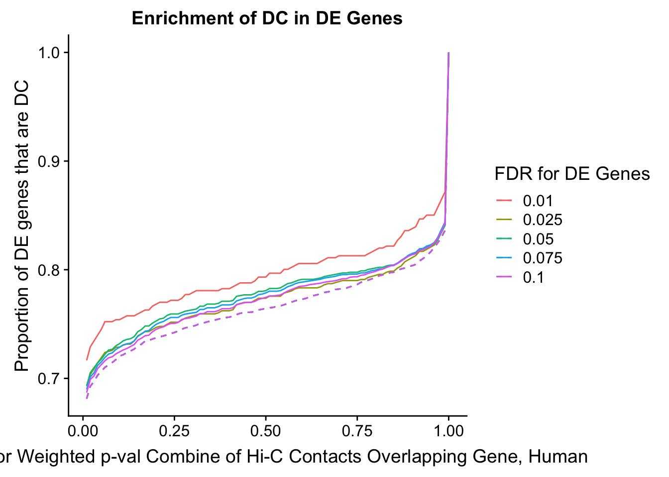
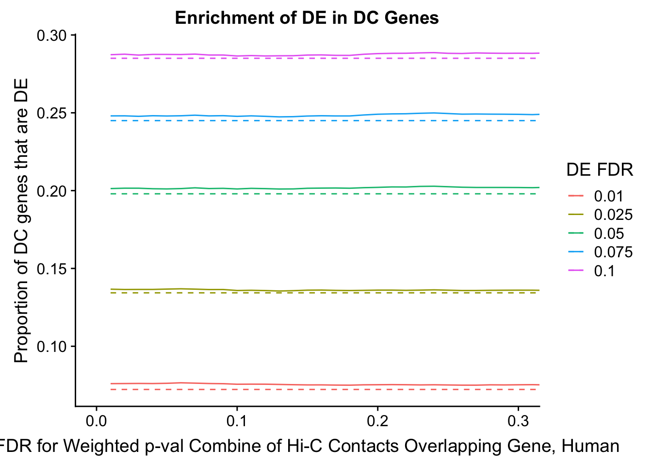
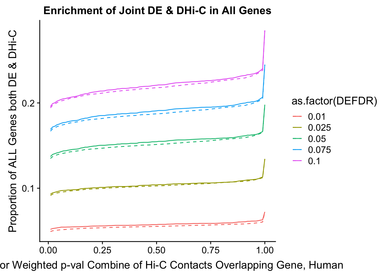
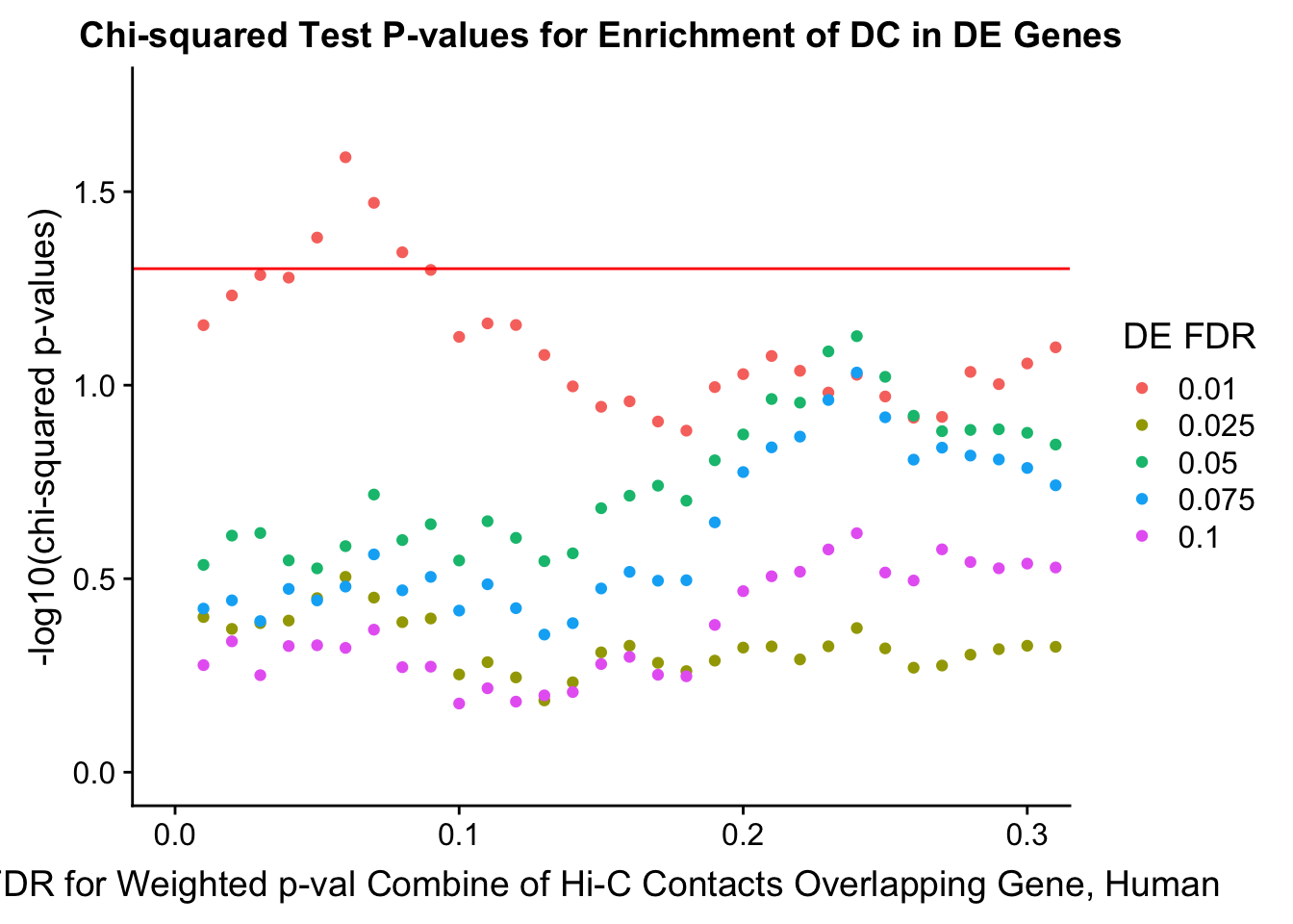
    DEFDR DHICFDR  prop.obs  prop.exp   chisq.p Dneither  DE DHiC Dboth
101 0.025    0.01 0.6931927 0.6813498 0.3972617     2154 320 4567   723
102 0.025    0.02 0.7037392 0.6926842 0.4262433     2077 309 4644   734
103 0.025    0.03 0.7085331 0.6971922 0.4119093     2047 304 4674   739
104 0.025    0.04 0.7142857 0.7028594 0.4057078     2009 298 4712   745
105 0.025    0.05 0.7190796 0.7064657 0.3549975     1986 293 4735   750
106 0.025    0.06 0.7238734 0.7102009 0.3127680     1962 288 4759   755
107 0.025    0.07 0.7248322 0.7122617 0.3538870     1947 287 4774   756
108 0.025    0.08 0.7257910 0.7145801 0.4094726     1930 286 4791   757
109 0.025    0.09 0.7286673 0.7172849 0.4006753     1912 283 4809   760
110 0.025    0.10 0.7286673 0.7206337 0.5589481     1886 283 4835   760
111 0.025    0.11 0.7305849 0.7217929 0.5196454     1879 281 4842   762
112 0.025    0.12 0.7315436 0.7237249 0.5688617     1865 280 4856   763
113 0.025    0.13 0.7315436 0.7252705 0.6523268     1853 280 4868   763
114 0.025    0.14 0.7344199 0.7269449 0.5857314     1843 277 4878   766
115 0.025    0.15 0.7392138 0.7299073 0.4901449     1825 272 4896   771
116 0.025    0.16 0.7411314 0.7314529 0.4712415     1815 270 4906   773
117 0.025    0.17 0.7430489 0.7344152 0.5215973     1794 268 4927   775
118 0.025    0.18 0.7430489 0.7349304 0.5479962     1790 268 4931   775
119 0.025    0.19 0.7449664 0.7362184 0.5148587     1782 266 4939   777
120 0.025    0.20 0.7468840 0.7373776 0.4764457     1775 264 4946   779
121 0.025    0.21 0.7478428 0.7382792 0.4731672     1769 263 4952   780
122 0.025    0.22 0.7478428 0.7390520 0.5112206     1763 263 4958   780
123 0.025    0.23 0.7497603 0.7402112 0.4728104     1756 261 4965   782
124 0.025    0.24 0.7516779 0.7411128 0.4241548     1751 259 4970   784
125 0.025    0.25 0.7516779 0.7422720 0.4786914     1742 259 4979   784
126 0.025    0.26 0.7516779 0.7434312 0.5370215     1733 259 4988   784
127 0.025    0.27 0.7535954 0.7452344 0.5300933     1721 257 5000   786
128 0.025    0.28 0.7555129 0.7465224 0.4970437     1713 255 5008   788
129 0.025    0.29 0.7564717 0.7471664 0.4808983     1709 254 5012   789
130 0.025    0.30 0.7574305 0.7479392 0.4712536     1704 253 5017   790
131 0.025    0.31 0.7583893 0.7489696 0.4741843     1697 252 5024   791
132 0.025    0.32 0.7593480 0.7506440 0.5093372     1685 251 5036   792
133 0.025    0.33 0.7593480 0.7510304 0.5292214     1682 251 5039   792
134 0.025    0.34 0.7593480 0.7520608 0.5842127     1674 251 5047   792
135 0.025    0.35 0.7593480 0.7528336 0.6272298     1668 251 5053   792
136 0.025    0.36 0.7593480 0.7536064 0.6716460     1662 251 5059   792
137 0.025    0.37 0.7603068 0.7545080 0.6679048     1656 250 5065   793
138 0.025    0.38 0.7622244 0.7552808 0.6017349     1652 248 5069   795
139 0.025    0.39 0.7622244 0.7559248 0.6381185     1647 248 5074   795
140 0.025    0.40 0.7622244 0.7563112 0.6604139     1644 248 5077   795
141 0.025    0.41 0.7631831 0.7572128 0.6566643     1638 247 5083   796
142 0.025    0.42 0.7679770 0.7587584 0.4783072     1631 242 5090   801
143 0.025    0.43 0.7689358 0.7599176 0.4877400     1623 241 5098   802
144 0.025    0.44 0.7698945 0.7604328 0.4650896     1620 240 5101   803
145 0.025    0.45 0.7698945 0.7608192 0.4842679     1617 240 5104   803
146 0.025    0.46 0.7698945 0.7609480 0.4907593     1616 240 5105   803
147 0.025    0.47 0.7718121 0.7614632 0.4214972     1614 238 5107   805
148 0.025    0.48 0.7737296 0.7630088 0.4031619     1604 236 5117   807
149 0.025    0.49 0.7737296 0.7636528 0.4329490     1599 236 5122   807
150 0.025    0.50 0.7737296 0.7642968 0.4640294     1594 236 5127   807
151 0.025    0.51 0.7756472 0.7649408 0.4024955     1591 234 5130   809
152 0.025    0.52 0.7756472 0.7653272 0.4202417     1588 234 5133   809
153 0.025    0.53 0.7756472 0.7664863 0.4762909     1579 234 5142   809
154 0.025    0.54 0.7756472 0.7667439 0.4893072     1577 234 5144   809
155 0.025    0.55 0.7785235 0.7677743 0.3985457     1572 231 5149   812
156 0.025    0.56 0.7794823 0.7689335 0.4069948     1564 230 5157   813
157 0.025    0.57 0.7804410 0.7700927 0.4155751     1556 229 5165   814
158 0.025    0.58 0.7823586 0.7713807 0.3855222     1548 227 5173   816
159 0.025    0.59 0.7833174 0.7721535 0.3765925     1543 226 5178   817
160 0.025    0.60 0.7833174 0.7727975 0.4055625     1538 226 5183   817
161 0.025    0.61 0.7833174 0.7736991 0.4483874     1531 226 5190   817
162 0.025    0.62 0.7833174 0.7749871 0.5140273     1521 226 5200   817
163 0.025    0.63 0.7833174 0.7761463 0.5773590     1512 226 5209   817
164 0.025    0.64 0.7833174 0.7769191 0.6216599     1506 226 5215   817
165 0.025    0.65 0.7842761 0.7780783 0.6328810     1498 225 5223   818
166 0.025    0.66 0.7861937 0.7791087 0.5804679     1492 223 5229   820
167 0.025    0.67 0.7871524 0.7796239 0.5549829     1489 222 5232   821
168 0.025    0.68 0.7871524 0.7803967 0.5987092     1483 222 5238   821
169 0.025    0.69 0.7881112 0.7818135 0.6248479     1473 221 5248   822
170 0.025    0.70 0.7890700 0.7821999 0.5909646     1471 220 5250   823
171 0.025    0.71 0.7900288 0.7827151 0.5651334     1468 219 5253   824
172 0.025    0.72 0.7900288 0.7831015 0.5870885     1465 219 5256   824
173 0.025    0.73 0.7900288 0.7842607 0.6553850     1456 219 5265   824
174 0.025    0.74 0.7900288 0.7852911 0.7188717     1448 219 5273   824
175 0.025    0.75 0.7900288 0.7864503 0.7929415     1439 219 5282   824
176 0.025    0.76 0.7909875 0.7883823 0.8566349     1425 218 5296   825
177 0.025    0.77 0.7909875 0.7892839 0.9170080     1418 218 5303   825
178 0.025    0.78 0.7929051 0.7904431 0.8657246     1411 216 5310   827
179 0.025    0.79 0.7938639 0.7916023 0.8789435     1403 215 5318   828
180 0.025    0.80 0.7948226 0.7931479 0.9184080     1392 214 5329   829
181 0.025    0.81 0.7957814 0.7944359 0.9406938     1383 213 5338   830
182 0.025    0.82 0.7957814 0.7953375 1.0000000     1376 213 5345   830
183 0.025    0.83 0.7976989 0.7962391 0.9326620     1371 211 5350   832
184 0.025    0.84 0.7986577 0.7972694 0.9374527     1364 210 5357   833
185 0.025    0.85 0.7986577 0.7977846 0.9728592     1360 210 5361   833
186 0.025    0.86 0.8015340 0.7994590 0.8899851     1350 207 5371   836
187 0.025    0.87 0.8034516 0.8007470 0.8466728     1342 205 5379   838
188 0.025    0.88 0.8072867 0.8015198 0.6454091     1340 201 5381   842
189 0.025    0.89 0.8092042 0.8029366 0.6134962     1331 199 5390   844
190 0.025    0.90 0.8111218 0.8037094 0.5445943     1327 197 5394   846
191 0.025    0.91 0.8130393 0.8048686 0.5005267     1320 195 5401   848
192 0.025    0.92 0.8168744 0.8080886 0.4640761     1299 191 5422   852
193 0.025    0.93 0.8168744 0.8102782 0.5881470     1282 191 5439   852
194 0.025    0.94 0.8187919 0.8129830 0.6351886     1263 189 5458   854
195 0.025    0.95 0.8207095 0.8162030 0.7181698     1240 187 5481   856
196 0.025    0.96 0.8226270 0.8201958 0.8599597     1211 185 5510   858
197 0.025    0.97 0.8274209 0.8247038 0.8381277     1181 180 5540   863
198 0.025    0.98 0.8350911 0.8297269 0.6519196     1150 172 5571   871
199 0.025    0.99 0.8427613 0.8362957 0.5744072     1107 164 5614   879
200 0.025    1.00 1.0000000 1.0000000 0.0000000        0   0 6721  1043
enrichment.plotter(gene.hic.filt, "weighted_Z.s2post.C", "adj.P.Val", "FDR for Weighted p-val Combine of Hi-C Contacts Overlapping Gene, Chimp")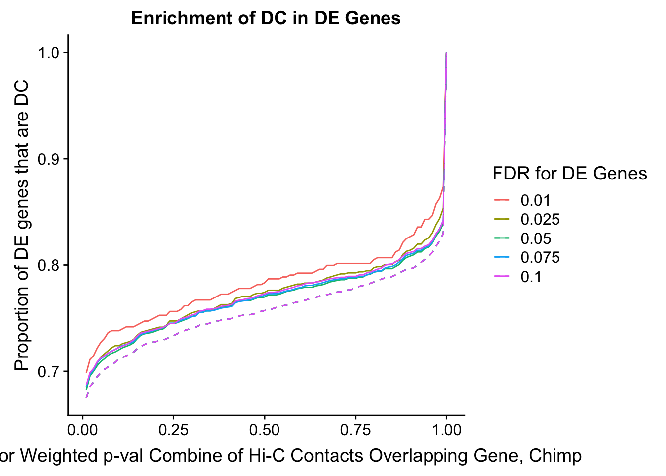
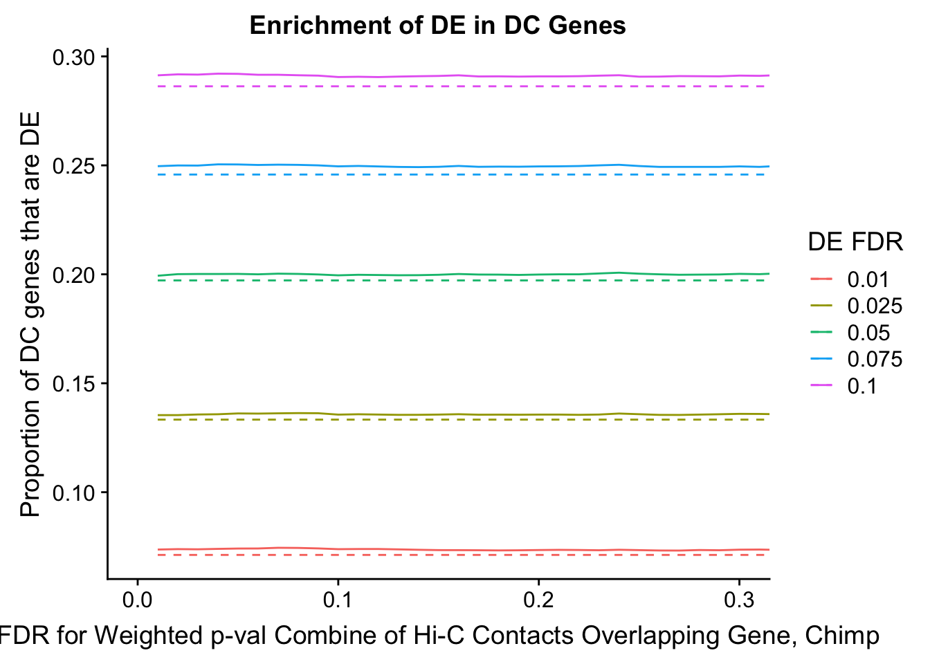

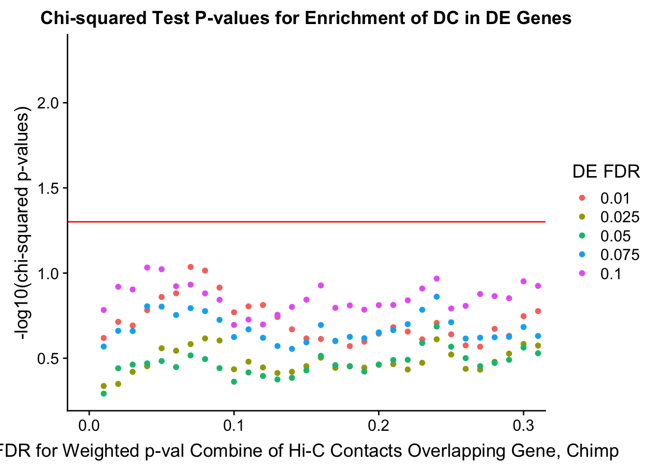
    DEFDR DHICFDR  prop.obs  prop.exp    chisq.p Dneither  DE DHiC Dboth
101 0.025    0.01 0.6856316 0.6751510 0.46021414     2201 326 4541   711
102 0.025    0.02 0.6962392 0.6855637 0.44760222     2131 315 4611   722
103 0.025    0.03 0.7020251 0.6898059 0.38011907     2104 309 4638   728
104 0.025    0.04 0.7078110 0.6949479 0.35230133     2070 303 4672   734
105 0.025    0.05 0.7135969 0.6986759 0.27636813     2047 297 4695   740
106 0.025    0.06 0.7164899 0.7018897 0.28570217     2025 294 4717   743
107 0.025    0.07 0.7193828 0.7040751 0.26122974     2011 291 4731   746
108 0.025    0.08 0.7222758 0.7063890 0.24198531     1996 288 4746   749
109 0.025    0.09 0.7242044 0.7085744 0.24888459     1981 286 4761   751
110 0.025    0.10 0.7242044 0.7119167 0.36720698     1955 286 4787   751
111 0.025    0.11 0.7261331 0.7129451 0.33129286     1949 284 4793   753
112 0.025    0.12 0.7270974 0.7146163 0.35805795     1937 283 4805   754
113 0.025    0.13 0.7280617 0.7162874 0.38623713     1925 282 4817   755
114 0.025    0.14 0.7299904 0.7180872 0.37991961     1913 280 4829   757
115 0.025    0.15 0.7338476 0.7213009 0.35197339     1892 276 4850   761
116 0.025    0.16 0.7367406 0.7232292 0.31376976     1880 273 4862   764
117 0.025    0.17 0.7377049 0.7254146 0.36009552     1864 272 4878   765
118 0.025    0.18 0.7386692 0.7261859 0.35187595     1859 271 4883   766
119 0.025    0.19 0.7396336 0.7273428 0.35902517     1851 270 4891   767
120 0.025    0.20 0.7405979 0.7279856 0.34573331     1847 269 4895   768
121 0.025    0.21 0.7415622 0.7288855 0.34267463     1841 268 4901   769
122 0.025    0.22 0.7415622 0.7295282 0.36835975     1836 268 4906   769
123 0.025    0.23 0.7434908 0.7306852 0.33658296     1829 266 4913   771
124 0.025    0.24 0.7473481 0.7319707 0.24473439     1823 262 4919   775
125 0.025    0.25 0.7473481 0.7336419 0.30077161     1810 262 4932   775
126 0.025    0.26 0.7473481 0.7353130 0.36502563     1797 262 4945   775
127 0.025    0.27 0.7492768 0.7373698 0.36917169     1783 260 4959   777
128 0.025    0.28 0.7512054 0.7383983 0.33203979     1777 258 4965   779
129 0.025    0.29 0.7531340 0.7394267 0.29732325     1771 256 4971   781
130 0.025    0.30 0.7550627 0.7403265 0.26079136     1766 254 4976   783
131 0.025    0.31 0.7560270 0.7414835 0.26659559     1758 253 4984   784
132 0.025    0.32 0.7569913 0.7432832 0.29495148     1745 252 4997   785
133 0.025    0.33 0.7569913 0.7436689 0.30901872     1742 252 5000   785
134 0.025    0.34 0.7579556 0.7444402 0.30132508     1737 251 5005   786
135 0.025    0.35 0.7579556 0.7454686 0.34043709     1729 251 5013   786
136 0.025    0.36 0.7589200 0.7463684 0.33728650     1723 250 5019   787
137 0.025    0.37 0.7608486 0.7473968 0.30183959     1717 248 5025   789
138 0.025    0.38 0.7627772 0.7480396 0.25603078     1714 246 5028   791
139 0.025    0.39 0.7627772 0.7486823 0.27768691     1709 246 5033   791
140 0.025    0.40 0.7627772 0.7490680 0.29128122     1706 246 5036   791
141 0.025    0.41 0.7637416 0.7497108 0.27929964     1702 245 5040   792
142 0.025    0.42 0.7685632 0.7512534 0.17813969     1695 240 5047   797
143 0.025    0.43 0.7695275 0.7521532 0.17595841     1689 239 5053   798
144 0.025    0.44 0.7704918 0.7526674 0.16442762     1686 238 5056   799
145 0.025    0.45 0.7704918 0.7531816 0.17699899     1682 238 5060   799
146 0.025    0.46 0.7704918 0.7533102 0.18025366     1681 238 5061   799
147 0.025    0.47 0.7724204 0.7539530 0.14862023     1678 236 5064   801
148 0.025    0.48 0.7733848 0.7553670 0.15823145     1668 235 5074   802
149 0.025    0.49 0.7733848 0.7563954 0.18345675     1660 235 5082   802
150 0.025    0.50 0.7743491 0.7571667 0.17791938     1655 234 5087   803
151 0.025    0.51 0.7762777 0.7579380 0.14927166     1651 232 5091   805
152 0.025    0.52 0.7762777 0.7585808 0.16408545     1646 232 5096   805
153 0.025    0.53 0.7762777 0.7598663 0.19708411     1636 232 5106   805
154 0.025    0.54 0.7762777 0.7606376 0.21914754     1630 232 5112   805
155 0.025    0.55 0.7782064 0.7616660 0.19233559     1624 230 5118   807
156 0.025    0.56 0.7791707 0.7623088 0.18317497     1620 229 5122   808
157 0.025    0.57 0.7801350 0.7633372 0.18423861     1613 228 5129   809
158 0.025    0.58 0.7810993 0.7643656 0.18530647     1606 227 5136   810
159 0.025    0.59 0.7820636 0.7652655 0.18298868     1600 226 5142   811
160 0.025    0.60 0.7820636 0.7657797 0.19683399     1596 226 5146   811
161 0.025    0.61 0.7830280 0.7666795 0.19441671     1590 225 5152   812
162 0.025    0.62 0.7830280 0.7678365 0.22816994     1581 225 5161   812
163 0.025    0.63 0.7830280 0.7686078 0.25294590     1575 225 5167   812
164 0.025    0.64 0.7839923 0.7695076 0.25011205     1569 224 5173   813
165 0.025    0.65 0.7849566 0.7707932 0.26020650     1560 223 5182   814
166 0.025    0.66 0.7859209 0.7715645 0.25297990     1555 222 5187   815
167 0.025    0.67 0.7878496 0.7720787 0.20742390     1553 220 5189   817
168 0.025    0.68 0.7888139 0.7728500 0.20120588     1548 219 5194   818
169 0.025    0.69 0.7897782 0.7740069 0.20605049     1540 218 5202   819
170 0.025    0.70 0.7907425 0.7745211 0.19265044     1537 217 5205   820
171 0.025    0.71 0.7917068 0.7749068 0.17653650     1535 216 5207   821
172 0.025    0.72 0.7917068 0.7752925 0.18671530     1532 216 5210   821
173 0.025    0.73 0.7926712 0.7765780 0.19484369     1523 215 5219   822
174 0.025    0.74 0.7926712 0.7770922 0.20958350     1519 215 5223   822
175 0.025    0.75 0.7926712 0.7783777 0.25004309     1509 215 5233   822
176 0.025    0.76 0.7936355 0.7799203 0.26922711     1498 214 5244   823
177 0.025    0.77 0.7936355 0.7806916 0.29752312     1492 214 5250   823
178 0.025    0.78 0.7945998 0.7817200 0.29919696     1485 213 5257   824
179 0.025    0.79 0.7945998 0.7827484 0.34025411     1477 213 5265   824
180 0.025    0.80 0.7974928 0.7841625 0.28002460     1469 210 5273   827
181 0.025    0.81 0.7984571 0.7857051 0.30098146     1458 209 5284   828
182 0.025    0.82 0.7984571 0.7866050 0.33708380     1451 209 5291   828
183 0.025    0.83 0.8003857 0.7878905 0.30940098     1443 207 5299   830
184 0.025    0.84 0.8003857 0.7885332 0.33546641     1438 207 5304   830
185 0.025    0.85 0.8003857 0.7891760 0.36296578     1433 207 5309   830
186 0.025    0.86 0.8032787 0.7907186 0.30441762     1424 204 5318   833
187 0.025    0.87 0.8042430 0.7926469 0.34299283     1410 203 5332   834
188 0.025    0.88 0.8100289 0.7943180 0.19249185     1403 197 5339   840
189 0.025    0.89 0.8129219 0.7959892 0.15792902     1393 194 5349   843
190 0.025    0.90 0.8138862 0.7963749 0.14352988     1391 193 5351   844
191 0.025    0.91 0.8158149 0.7975318 0.12544667     1384 191 5358   846
192 0.025    0.92 0.8196721 0.8001028 0.09875858     1368 187 5374   850
193 0.025    0.93 0.8196721 0.8025453 0.14808855     1349 187 5393   850
194 0.025    0.94 0.8235294 0.8051163 0.11739041     1333 183 5409   854
195 0.025    0.95 0.8254581 0.8082016 0.14055283     1311 181 5431   856
196 0.025    0.96 0.8302797 0.8119296 0.11372824     1287 176 5455   861
197 0.025    0.97 0.8379942 0.8175858 0.07429587     1251 168 5491   869
198 0.025    0.98 0.8437801 0.8227279 0.06244267     1217 162 5525   875
199 0.025    0.99 0.8534233 0.8295411 0.03135694     1174 152 5568   885
200 0.025    1.00 1.0000000 1.0000000 0.00000000        0   0 6742  1037
#FIG4B
enrichment.plotter(gene.hic.filt, "weighted_Z.ALLvar.H", "adj.P.Val", "FDR for Weighted p-val Combine of Hi-C Contacts Overlapping Gene", xmax=1) #FIG4BWarning in chisq.test(mytable): Chi-squared approximation may be incorrect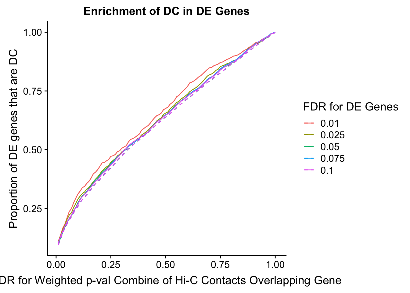
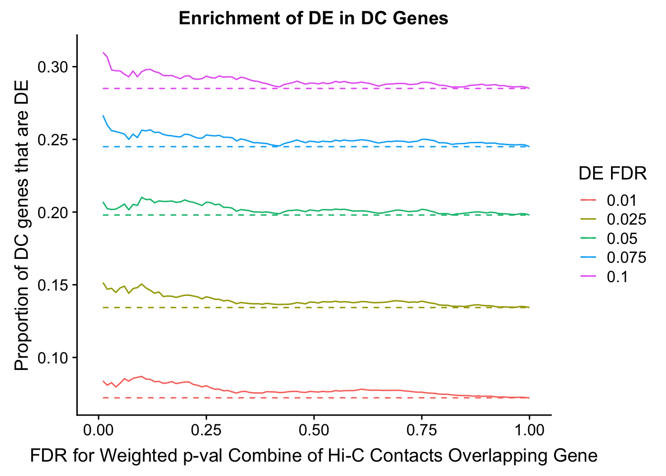
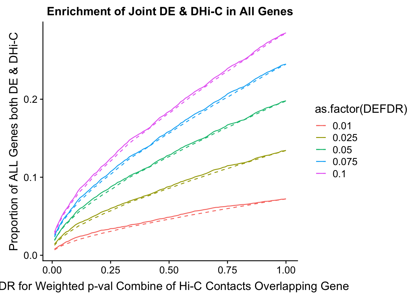
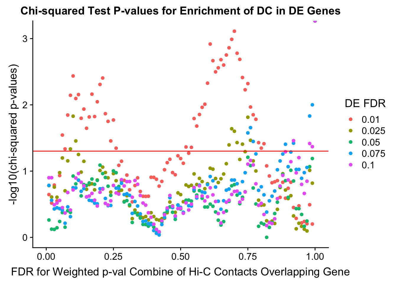
    DEFDR DHICFDR  prop.obs  prop.exp    chisq.p Dneither  DE DHiC Dboth
101 0.025    0.01 0.1073826 0.0951829 0.16566657     6094 931  627   112
102 0.025    0.02 0.1323106 0.1209428 0.24639993     5920 905  801   138
103 0.025    0.03 0.1591563 0.1448995 0.17427317     5762 877  959   166
104 0.025    0.04 0.1792905 0.1664091 0.24774781     5616 856 1105   187
105 0.025    0.05 0.2032598 0.1846986 0.10579031     5499 831 1222   212
106 0.025    0.06 0.2224353 0.2005410 0.06338830     5396 811 1325   232
107 0.025    0.07 0.2310642 0.2153529 0.19837106     5290 802 1431   241
108 0.025    0.08 0.2540748 0.2315817 0.07008123     5188 778 1533   265
109 0.025    0.09 0.2713327 0.2461360 0.04639849     5093 760 1628   283
110 0.025    0.10 0.2905081 0.2592736 0.01485043     5011 740 1710   303
111 0.025    0.11 0.3029722 0.2753735 0.03509085     4899 727 1822   316
112 0.025    0.12 0.3135187 0.2881247 0.05619163     4811 716 1910   327
113 0.025    0.13 0.3202301 0.2982998 0.10363917     4739 709 1982   334
114 0.025    0.14 0.3326942 0.3082174 0.07124345     4675 696 2046   347
115 0.025    0.15 0.3394056 0.3212262 0.18825806     4581 689 2140   354
116 0.025    0.16 0.3518696 0.3323029 0.15956077     4508 676 2213   367
117 0.025    0.17 0.3643337 0.3444101 0.15549829     4427 663 2294   380
118 0.025    0.18 0.3748802 0.3563885 0.19173623     4345 652 2376   391
119 0.025    0.19 0.3844679 0.3633436 0.13624023     4301 642 2420   401
120 0.025    0.20 0.3969319 0.3733900 0.09792680     4236 629 2485   414
121 0.025    0.21 0.4103547 0.3858836 0.08713408     4153 615 2568   428
122 0.025    0.22 0.4189837 0.3956723 0.10507811     4086 606 2635   437
123 0.025    0.23 0.4266539 0.4045595 0.12634723     4025 598 2696   445
124 0.025    0.24 0.4333653 0.4149923 0.20746512     3951 591 2770   452
125 0.025    0.25 0.4467881 0.4234930 0.10898156     3899 577 2822   466
126 0.025    0.26 0.4544583 0.4328954 0.13966930     3834 569 2887   474
127 0.025    0.27 0.4621285 0.4434570 0.20369707     3760 561 2961   482
128 0.025    0.28 0.4736337 0.4545337 0.19426645     3686 549 3035   494
129 0.025    0.29 0.4803452 0.4645801 0.28740313     3615 542 3106   501
130 0.025    0.30 0.4908917 0.4733385 0.23523257     3558 531 3163   512
131 0.025    0.31 0.4985618 0.4841577 0.33345645     3482 523 3239   520
132 0.025    0.32 0.5043145 0.4945904 0.52098840     3407 517 3314   526
133 0.025    0.33 0.5167785 0.5038640 0.38797232     3348 504 3373   539
134 0.025    0.34 0.5234899 0.5117208 0.43305399     3294 497 3427   546
135 0.025    0.35 0.5311601 0.5204791 0.47844162     3234 489 3487   554
136 0.025    0.36 0.5378715 0.5278207 0.50573082     3184 482 3537   561
137 0.025    0.37 0.5455417 0.5350335 0.48521579     3136 474 3585   569
138 0.025    0.38 0.5512943 0.5421175 0.54454660     3087 468 3634   575
139 0.025    0.39 0.5627996 0.5508758 0.42449961     3031 456 3690   587
140 0.025    0.40 0.5685523 0.5580886 0.48526872     2981 450 3740   593
141 0.025    0.41 0.5752637 0.5659454 0.53590184     2927 443 3794   600
142 0.025    0.42 0.5829338 0.5739310 0.54964267     2873 435 3848   608
143 0.025    0.43 0.5925216 0.5829469 0.52198812     2813 425 3908   618
144 0.025    0.44 0.6011505 0.5914477 0.51485525     2756 416 3965   627
145 0.025    0.45 0.6116970 0.5999485 0.42461271     2701 405 4020   638
146 0.025    0.46 0.6232023 0.6079341 0.29304502     2651 393 4070   650
147 0.025    0.47 0.6299137 0.6159196 0.33479652     2596 386 4125   657
148 0.025    0.48 0.6356663 0.6239052 0.41884916     2540 380 4181   663
149 0.025    0.49 0.6500479 0.6322772 0.21322226     2490 365 4231   678
150 0.025    0.50 0.6558006 0.6385884 0.22666331     2447 359 4274   684
151 0.025    0.51 0.6605944 0.6455435 0.29034101     2398 354 4323   689
152 0.025    0.52 0.6730585 0.6534003 0.16184419     2350 341 4371   702
153 0.025    0.53 0.6816874 0.6625451 0.17067444     2288 332 4433   711
154 0.025    0.54 0.6893576 0.6700155 0.16378147     2238 324 4483   719
155 0.025    0.55 0.7008629 0.6789026 0.11027142     2181 312 4540   731
156 0.025    0.56 0.7056568 0.6863730 0.15947943     2128 307 4593   736
157 0.025    0.57 0.7152445 0.6946162 0.12887998     2074 297 4647   746
158 0.025    0.58 0.7219559 0.7022154 0.14372584     2022 290 4699   753
159 0.025    0.59 0.7286673 0.7108449 0.18423758     1962 283 4759   760
160 0.025    0.60 0.7363375 0.7174137 0.15505243     1919 275 4802   768
161 0.025    0.61 0.7468840 0.7246265 0.09059411     1874 264 4847   779
162 0.025    0.62 0.7535954 0.7317105 0.09355014     1826 257 4895   786
163 0.025    0.63 0.7593480 0.7396960 0.12935779     1770 251 4951   792
164 0.025    0.64 0.7651007 0.7465224 0.14868182     1723 245 4998   798
165 0.025    0.65 0.7737296 0.7545080 0.13063361     1670 236 5051   807
166 0.025    0.66 0.7813998 0.7613344 0.11073551     1625 228 5096   815
167 0.025    0.67 0.7909875 0.7690623 0.07733338     1575 218 5146   825
168 0.025    0.68 0.8024928 0.7774343 0.04026349     1522 206 5199   837
169 0.025    0.69 0.8130393 0.7856775 0.02296910     1469 195 5252   848
170 0.025    0.70 0.8187919 0.7921175 0.02504537     1425 189 5296   854
171 0.025    0.71 0.8226270 0.7980422 0.03714207     1383 185 5338   858
172 0.025    0.72 0.8283797 0.8070582 0.06675188     1319 179 5402   864
173 0.025    0.73 0.8379674 0.8143998 0.03927027     1272 169 5449   874
174 0.025    0.74 0.8427613 0.8207110 0.05094645     1228 164 5493   879
175 0.025    0.75 0.8542665 0.8274086 0.01539372     1188 152 5533   891
176 0.025    0.76 0.8571429 0.8339773 0.03432323     1140 149 5581   894
177 0.025    0.77 0.8609779 0.8414477 0.07022857     1086 145 5635   898
178 0.025    0.78 0.8657718 0.8482741 0.09964101     1038 140 5683   903
179 0.025    0.79 0.8686481 0.8571613 0.27485605      972 137 5749   906
180 0.025    0.80 0.8744008 0.8642452 0.32680957      923 131 5798   912
181 0.025    0.81 0.8791946 0.8691396 0.32434551      890 126 5831   917
182 0.025    0.82 0.8820709 0.8760948 0.56252048      839 123 5882   920
183 0.025    0.83 0.8878236 0.8824060 0.59464098      796 117 5925   926
184 0.025    0.84 0.8954938 0.8898764 0.56886945      746 109 5975   934
185 0.025    0.85 0.9022052 0.8973467 0.61649707      695 102 6026   941
186 0.025    0.86 0.9127517 0.9048171 0.37788876      648  91 6073   952
187 0.025    0.87 0.9242570 0.9128027 0.17692208      598  79 6123   964
188 0.025    0.88 0.9319271 0.9188563 0.10945665      559  71 6162   972
189 0.025    0.89 0.9367210 0.9264554 0.19313941      505  66 6216   977
190 0.025    0.90 0.9424736 0.9339258 0.25956552      453  60 6268   983
191 0.025    0.91 0.9491850 0.9406234 0.23519006      408  53 6313   990
192 0.025    0.92 0.9530201 0.9479650 0.47452447      355  49 6366   994
193 0.025    0.93 0.9568552 0.9544049 0.74295051      309  45 6412   998
194 0.025    0.94 0.9645254 0.9612313 0.61277921      264  37 6457  1006
195 0.025    0.95 0.9712368 0.9687017 0.68194799      213  30 6508  1013
196 0.025    0.96 0.9760307 0.9741113 0.75294672      176  25 6545  1018
197 0.025    0.97 0.9817833 0.9802937 0.80080639      134  19 6587  1024
198 0.025    0.98 0.9932886 0.9875064 0.09749270       90   7 6631  1036
199 0.025    0.99 0.9961649 0.9920144 0.15222995       58   4 6663  1039
200 0.025    1.00 1.0000000 1.0000000 0.00000000        0   0 6721  1043
enrichment.plotter(gene.hic.filt, "weighted_Z.ALLvar.C", "adj.P.Val", "FDR for Weighted p-val Combine of Hi-C Contacts Overlapping Gene, Chimp")Warning in chisq.test(mytable): Chi-squared approximation may be incorrect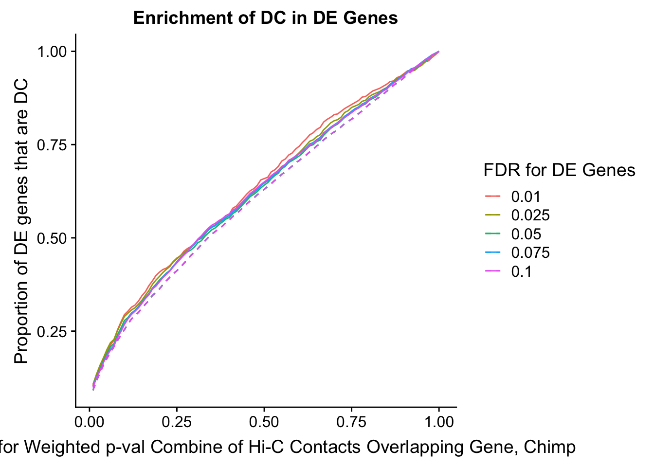
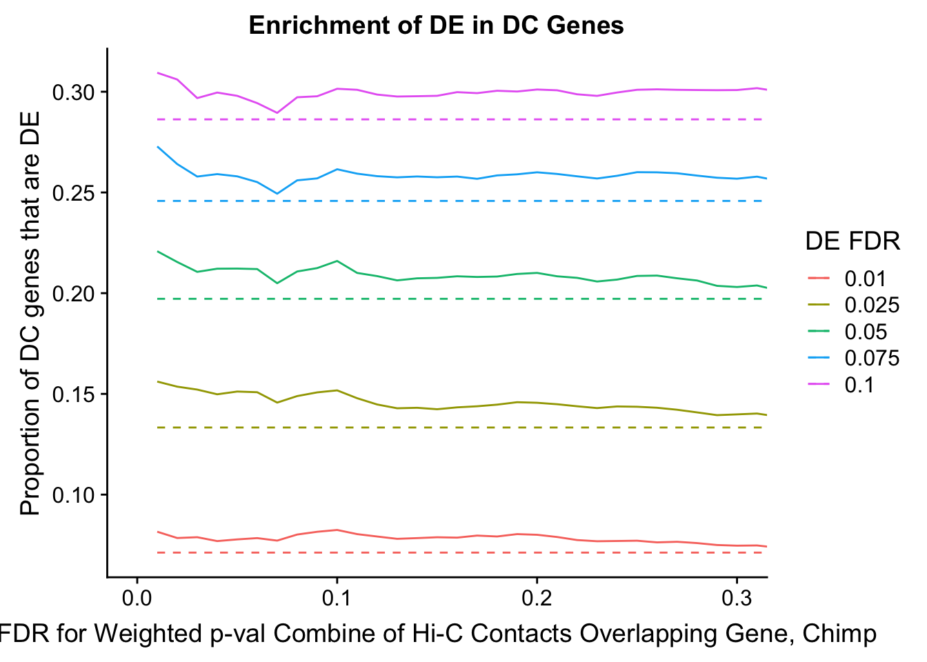
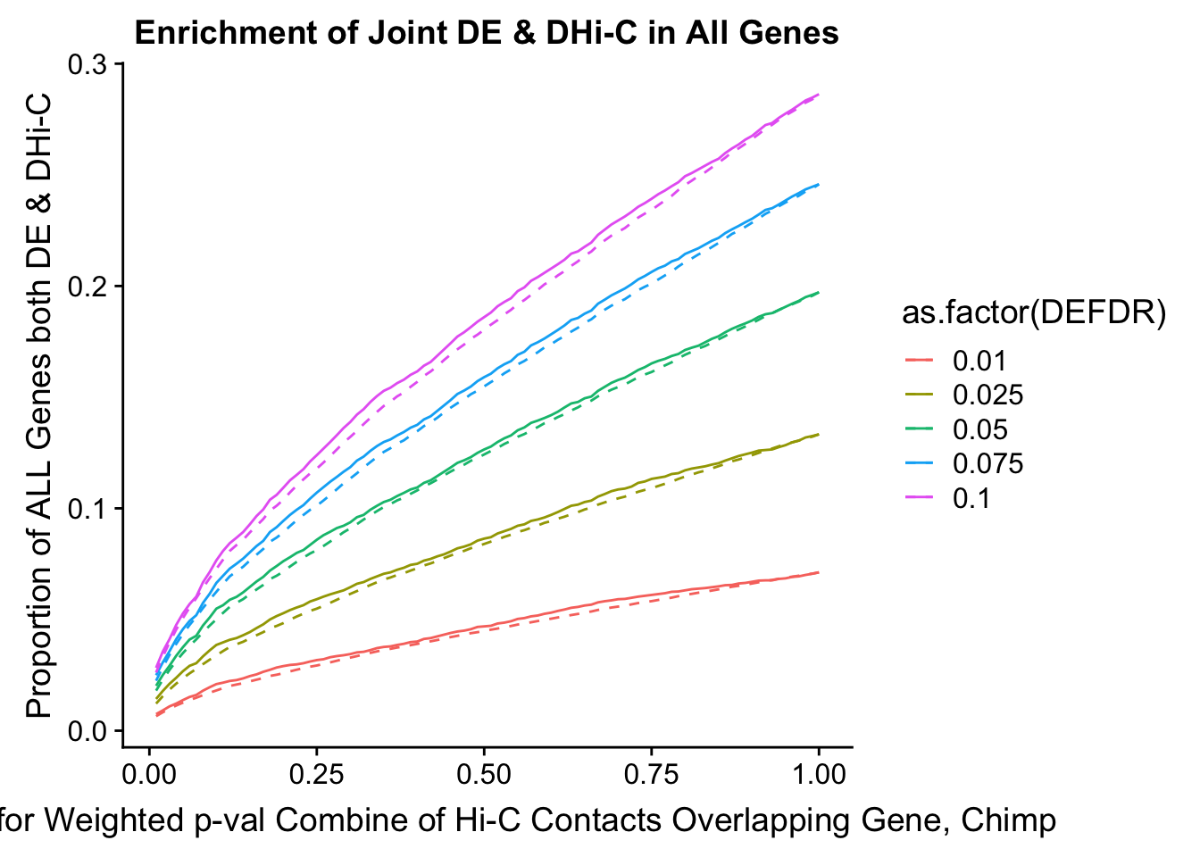
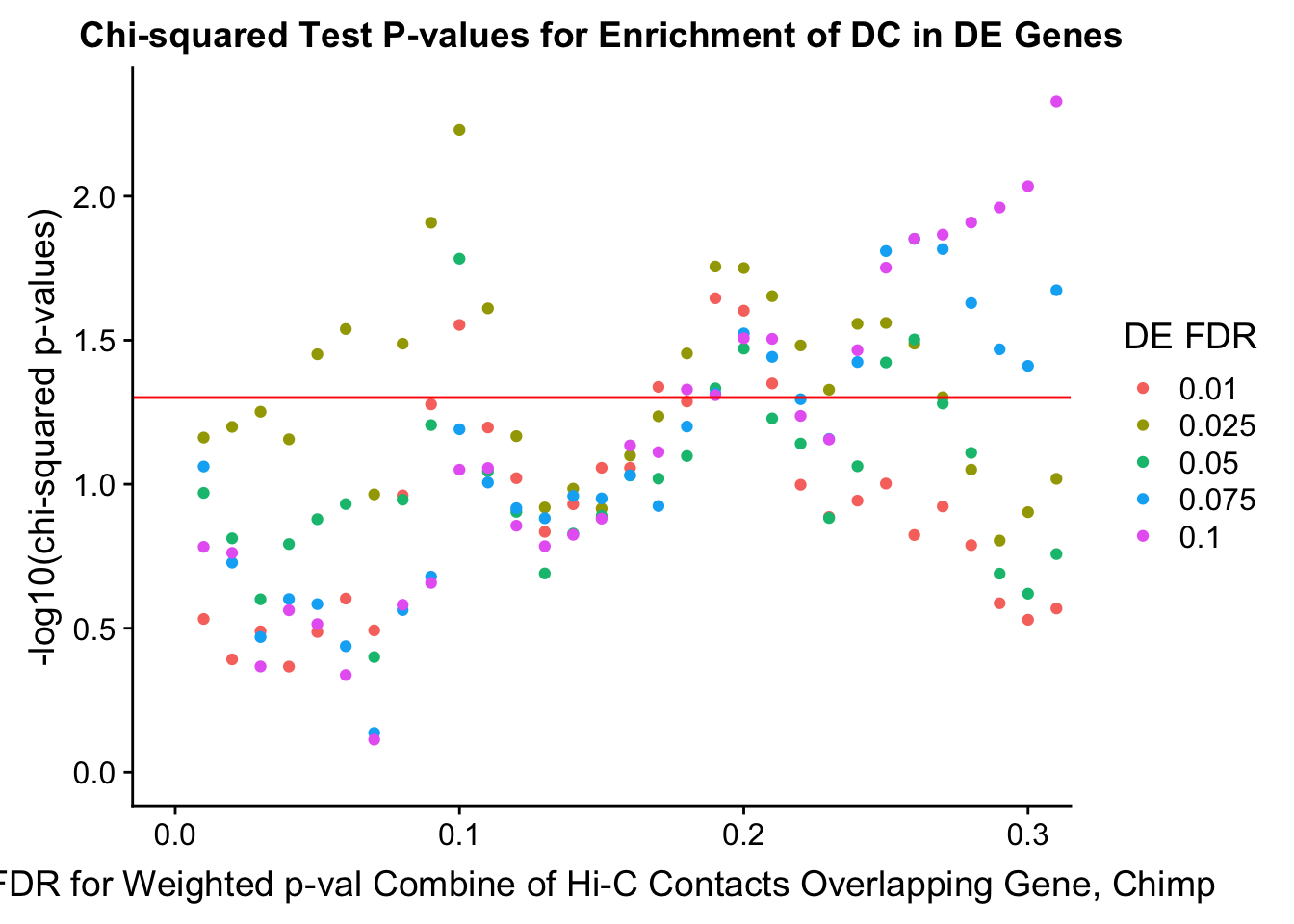
    DEFDR DHICFDR  prop.obs   prop.exp     chisq.p Dneither  DE DHiC Dboth
101 0.025    0.01 0.1070395 0.09139992 0.068853196     6142 926  600   111
102 0.025    0.02 0.1340405 0.11633886 0.063214019     5976 898  766   139
103 0.025    0.03 0.1581485 0.13857822 0.056002329     5828 873  914   164
104 0.025    0.04 0.1783992 0.15876077 0.069806446     5692 852 1050   185
105 0.025    0.05 0.2005786 0.17688649 0.035375055     5574 829 1168   208
106 0.025    0.06 0.2189007 0.19346960 0.028910832     5464 810 1278   227
107 0.025    0.07 0.2275796 0.20825299 0.108432406     5358 801 1384   236
108 0.025    0.08 0.2507232 0.22445044 0.032498272     5256 777 1486   260
109 0.025    0.09 0.2709740 0.23961949 0.012356986     5159 756 1583   281
110 0.025    0.10 0.2892960 0.25414578 0.005880942     5065 737 1677   300
111 0.025    0.11 0.2979749 0.26867207 0.024510965     4961 728 1781   309
112 0.025    0.12 0.3066538 0.28242705 0.068081758     4863 719 1879   318
113 0.025    0.13 0.3124397 0.29155418 0.120444739     4798 713 1944   324
114 0.025    0.14 0.3220829 0.30003857 0.103628174     4742 703 2000   334
115 0.025    0.15 0.3326905 0.31147962 0.121550116     4664 692 2078   345
116 0.025    0.16 0.3461909 0.32202083 0.079496527     4596 678 2146   359
117 0.025    0.17 0.3587271 0.33243347 0.058057354     4528 665 2214   372
118 0.025    0.18 0.3751205 0.34567425 0.035150264     4442 648 2300   389
119 0.025    0.19 0.3866924 0.35338732 0.017543076     4394 636 2348   401
120 0.025    0.20 0.3963356 0.36290012 0.017759159     4330 626 2412   411
121 0.025    0.21 0.4069431 0.37446973 0.022229963     4251 615 2491   422
122 0.025    0.22 0.4156220 0.38513948 0.032967045     4177 606 2565   431
123 0.025    0.23 0.4233365 0.39478082 0.046961821     4110 598 2632   439
124 0.025    0.24 0.4358727 0.40416506 0.027734682     4050 585 2692   452
125 0.025    0.25 0.4435873 0.41174958 0.027538008     3999 577 2743   460
126 0.025    0.26 0.4522662 0.42126237 0.032500938     3934 568 2808   469
127 0.025    0.27 0.4599807 0.43141792 0.049857681     3863 560 2879   477
128 0.025    0.28 0.4667310 0.44183057 0.088975524     3789 553 2953   484
129 0.025    0.29 0.4734812 0.45262887 0.156893824     3712 546 3030   491
130 0.025    0.30 0.4840887 0.46149891 0.125033582     3654 535 3088   502
131 0.025    0.31 0.4956606 0.47114025 0.095761121     3591 523 3151   514
132 0.025    0.32 0.5014465 0.48168145 0.181907573     3515 517 3227   520
133 0.025    0.33 0.5120540 0.49145134 0.163873995     3450 506 3292   531
134 0.025    0.34 0.5207329 0.50096413 0.182115992     3385 497 3357   540
135 0.025    0.35 0.5294118 0.51009127 0.192397158     3323 488 3419   549
136 0.025    0.36 0.5342334 0.51690449 0.243557982     3275 483 3467   554
137 0.025    0.37 0.5429122 0.52526032 0.234305586     3219 474 3523   563
138 0.025    0.38 0.5496625 0.53130222 0.215250651     3179 467 3563   570
139 0.025    0.39 0.5593057 0.54017226 0.195493243     3120 457 3622   580
140 0.025    0.40 0.5631630 0.54801388 0.308020850     3063 453 3679   584
141 0.025    0.41 0.5737705 0.55739812 0.268459804     3001 442 3741   595
142 0.025    0.42 0.5795564 0.56433989 0.304004528     2953 436 3789   601
143 0.025    0.43 0.5882353 0.57269572 0.292398396     2897 427 3845   610
144 0.025    0.44 0.5949855 0.58233706 0.393477739     2829 420 3913   617
145 0.025    0.45 0.6046287 0.59107854 0.357864220     2771 410 3971   627
146 0.025    0.46 0.6152363 0.59917727 0.271564608     2719 399 4023   638
147 0.025    0.47 0.6210222 0.60663324 0.324751980     2667 393 4075   644
148 0.025    0.48 0.6287367 0.61563183 0.369405642     2605 385 4137   652
149 0.025    0.49 0.6412729 0.62218794 0.184442385     2567 372 4175   665
150 0.025    0.50 0.6480231 0.63002957 0.209614647     2513 365 4229   672
151 0.025    0.51 0.6528447 0.63787119 0.296965338     2457 360 4285   677
152 0.025    0.52 0.6653809 0.64507006 0.151735391     2414 347 4328   690
153 0.025    0.53 0.6730955 0.65394010 0.174531621     2353 339 4389   698
154 0.025    0.54 0.6808100 0.66113896 0.160817050     2305 331 4437   706
155 0.025    0.55 0.6914176 0.67026610 0.128305720     2245 320 4497   717
156 0.025    0.56 0.6962392 0.67656511 0.155857310     2201 315 4541   722
157 0.025    0.57 0.7078110 0.68466384 0.091549698     2150 303 4592   734
158 0.025    0.58 0.7126326 0.69250546 0.140865172     2094 298 4648   739
159 0.025    0.59 0.7193828 0.70124695 0.182157727     2033 291 4709   746
160 0.025    0.60 0.7280617 0.70728885 0.122942868     1995 282 4747   755
161 0.025    0.61 0.7377049 0.71525903 0.092283471     1943 272 4799   765
162 0.025    0.62 0.7483124 0.72207225 0.046712056     1901 261 4841   776
163 0.025    0.63 0.7589200 0.73029952 0.028298505     1848 250 4894   787
164 0.025    0.64 0.7627772 0.73736984 0.050088057     1797 246 4945   791
165 0.025    0.65 0.7714561 0.74636843 0.050442569     1736 237 5006   800
166 0.025    0.66 0.7762777 0.75279599 0.065152590     1691 232 5051   805
167 0.025    0.67 0.7897782 0.76269443 0.030549193     1628 218 5114   819
168 0.025    0.68 0.7984571 0.77027896 0.022759294     1578 209 5164   828
169 0.025    0.69 0.8081003 0.77773493 0.012912256     1530 199 5212   838
170 0.025    0.70 0.8138862 0.78377684 0.012794712     1489 193 5253   844
171 0.025    0.71 0.8167792 0.78956164 0.023283223     1447 190 5295   847
172 0.025    0.72 0.8235294 0.79778892 0.029609167     1390 183 5352   854
173 0.025    0.73 0.8360656 0.80614475 0.009997835     1338 170 5404   867
174 0.025    0.74 0.8408872 0.81244376 0.013222715     1294 165 5448   872
175 0.025    0.75 0.8495661 0.81810001 0.005465053     1259 156 5483   881
176 0.025    0.76 0.8534233 0.82568454 0.012949356     1204 152 5538   885
177 0.025    0.77 0.8572806 0.83314051 0.028176325     1150 148 5592   889
178 0.025    0.78 0.8659595 0.84021082 0.017067390     1104 139 5638   898
179 0.025    0.79 0.8688525 0.84946651 0.067461266     1035 136 5707   901
180 0.025    0.80 0.8784957 0.85743669 0.041772820      983 126 5759   911
181 0.025    0.81 0.8842816 0.86412135 0.046984011      937 120 5805   917
182 0.025    0.82 0.8881389 0.87157732 0.096419716      883 116 5859   921
183 0.025    0.83 0.8919961 0.87736213 0.135609405      842 112 5900   925
184 0.025    0.84 0.8977821 0.88494665 0.180521043      789 106 5953   931
185 0.025    0.85 0.9026037 0.89253117 0.284116150      735 101 6007   936
186 0.025    0.86 0.9112825 0.90011570 0.217726259      685  92 6057   945
187 0.025    0.87 0.9189971 0.90898573 0.251799329      624  84 6118   953
188 0.025    0.88 0.9267117 0.91489909 0.160143564      586  76 6156   961
189 0.025    0.89 0.9324976 0.92196940 0.195124167      537  70 6205   967
190 0.025    0.90 0.9382835 0.92955393 0.264922383      484  64 6258   973
191 0.025    0.91 0.9450338 0.93726700 0.298730434      431  57 6311   980
192 0.025    0.92 0.9469624 0.94575138 0.911375049      367  55 6375   982
193 0.025    0.93 0.9488910 0.95192184 0.680273268      321  53 6421   984
194 0.025    0.94 0.9566056 0.95963491 0.654391822      269  45 6473   992
195 0.025    0.95 0.9633558 0.96657668 0.598155106      222  38 6520   999
196 0.025    0.96 0.9729990 0.97261859 1.000000000      185  28 6557  1009
197 0.025    0.97 0.9787850 0.97891760 1.000000000      142  22 6600  1015
198 0.025    0.98 0.9893925 0.98675922 0.515072513       92  11 6650  1026
199 0.025    0.99 0.9942141 0.99190127 0.479870616       57   6 6685  1031
200 0.025    1.00 1.0000000 1.00000000 0.000000000        0   0 6742  1037
#Custom function for doing this for the paper:
pap.enrichment.plotter <- function(df, HiC_col, DE_col, xlab, xmax=0.3, i=c(0.01, 0.025, 0.05, 0.075, 0.1), k=seq(0.01, 1, 0.01), significance=FALSE){
enrich.table <- data.frame(DEFDR = c(rep(i[1], 100), rep(i[2], 100), rep(i[3], 100), rep(i[4], 100), rep(i[5], 100)), DHICFDR=rep(k, 5), prop.obs=NA, prop.exp=NA, chisq.p=NA, Dneither=NA, DE=NA, DHiC=NA, Dboth=NA)
for(de.FDR in i){
for(hic.FDR in k){
enrich.table[which(enrich.table$DEFDR==de.FDR&enrich.table$DHICFDR==hic.FDR), 3:9] <- prop.calculator(df[,DE_col], df[,HiC_col], de.FDR, hic.FDR)
}
}
des.enriched <- ggplot(data=enrich.table, aes(x=DHICFDR, y=prop.obs, group=as.factor(DEFDR), color=as.factor(DEFDR))) +geom_line()+ geom_line(aes(y=prop.exp), linetype="dashed", size=0.5) + ggtitle("Enrichment of DC in DE Genes") + xlab(xlab) + ylab("Proportion of DE genes that are DC") + guides(color=guide_legend(title="FDR for DE Genes"))
dhics.enriched <- ggplot(data=enrich.table, aes(x=DHICFDR, y=Dboth/(Dboth+DHiC), group=as.factor(DEFDR), color=as.factor(DEFDR))) + geom_line() + geom_line(aes(y=(((((DE+Dboth)/(Dneither+DE+DHiC+Dboth))*((DHiC+Dboth)/(Dneither+DE+DHiC+Dboth)))*(Dneither+DE+DHiC+Dboth))/(DHiC+Dboth))), linetype="dashed") + ylab("Proportion of DC genes that are DE") +xlab(xlab) + ggtitle("Enrichment of DE in DC Genes") + coord_cartesian(xlim=c(0, xmax), ylim=c(0.05, 0.32)) + guides(color=FALSE)
joint.enriched <- ggplot(data=enrich.table, aes(x=DHICFDR, y=Dboth/(Dneither+DE+DHiC+Dboth), group=as.factor(DEFDR), color=as.factor(DEFDR))) + geom_line() + ylab("Proportion of ALL Genes both DE & DHi-C") + xlab(xlab) + geom_line(aes(y=((DE+Dboth)/(Dneither+DE+DHiC+Dboth))*((DHiC+Dboth)/(Dneither+DE+DHiC+Dboth))), linetype="dashed") + ggtitle("Enrichment of Joint DE & DHi-C in All Genes")
chisq.p <- ggplot(data=enrich.table, aes(x=DHICFDR, y=-log10(chisq.p), group=as.factor(DEFDR), color=as.factor(DEFDR))) + geom_point() + geom_hline(yintercept=-log10(0.05), color="red") + ggtitle("Chi-squared Test P-values") + xlab(xlab) + ylab("-log10(chi-squared p-values)") + coord_cartesian(xlim=c(0, xmax), ylim=c(0, 3.2)) + guides(color=guide_legend(title="DE FDR"))
if(significance==TRUE){
return(chisq.p)
}
else{
return(dhics.enriched)
}
}
#FIG4
FIG4A <- pap.enrichment.plotter(gene.hic.filt, "min_FDR.H", "adj.P.Val", "Minimum FDR of Contacts", xmax=1) #FIG4AWarning in chisq.test(mytable): Chi-squared approximation may be incorrect
Warning in chisq.test(mytable): Chi-squared approximation may be incorrect
Warning in chisq.test(mytable): Chi-squared approximation may be incorrectFIG4B <- pap.enrichment.plotter(gene.hic.filt, "min_FDR.H", "adj.P.Val", "Minimum FDR of Contacts", xmax=1, significance = TRUE) #FIG4BWarning in chisq.test(mytable): Chi-squared approximation may be incorrect
Warning in chisq.test(mytable): Chi-squared approximation may be incorrect
Warning in chisq.test(mytable): Chi-squared approximation may be incorrectFIG4C <- pap.enrichment.plotter(gene.hic.filt, "weighted_Z.ALLvar.H", "adj.P.Val", "FDR for Weighted P-val Combination", xmax=1) #FIG4CWarning in chisq.test(mytable): Chi-squared approximation may be incorrectFIG4D <- pap.enrichment.plotter(gene.hic.filt, "weighted_Z.ALLvar.H", "adj.P.Val", "FDR for Weighted P-val Combination", xmax=1, significance = TRUE) #FIG4DWarning in chisq.test(mytable): Chi-squared approximation may be incorrectFIG4 <- plot_grid(FIG4A, FIG4B, FIG4C, FIG4D, labels=c("A", "B", "C", "D"), align="h", rel_widths=c(1, 1.2))
save_plot("~/Desktop/FIG4.png", FIG4, nrow=2, ncol=2)Now that I’ve seen some enrichment of differential contact (DC) in differential expression (DE) based on my linear modeling results from before, I would like to further quantify this effect. In order to do so, I now extract log2 observed/expected homer-normalized contact frequency values and RPKM expression values for each gene/bin set, so I can look at correlations of these values and assess their explanatory power.
Contact Frequency Extraction
In this section, I proceed to create a function in order to extract the Hi-C interaction frequency values for the different types of summaries I’ve made gene overlaps with above. This allows for operations to be performed separately utilizing different summaries of Hi-C contacts.
#Get a df with the H and C coordinates of the hits, and the IF values from homer. This subset df makes things easier to extract.
contacts <- data.frame(h1=data.filtered$H1, h2=data.filtered$H2, c1=data.filtered$C1, c2=data.filtered$C2, A_21792_HIC=data.filtered$`A-21792_norm`, B_28126_HIC=data.filtered$`B-28126_norm`, C_3649_HIC=data.filtered$`C-3649_norm`, D_40300_HIC=data.filtered$`D-40300_norm`, E_28815_HIC=data.filtered$`E-28815_norm`, F_28834_HIC=data.filtered$`F-28834_norm`, G_3624_HIC=data.filtered$`G-3624_norm`, H_3651_HIC=data.filtered$`H-3651_norm`, stringsAsFactors = FALSE)

#Now ensure first member of a pair is always lower than second:
newH1 <- as.numeric(gsub(".*-", "", contacts$h1))
newH2 <- as.numeric(gsub(".*-", "", contacts$h2))
lower.HID <- ifelse(newH1<newH2, contacts$h1, contacts$h2)
higher.HID2 <- ifelse(newH1<newH2, contacts$h2, contacts$h1)
contacts$hpair <- paste(lower.HID, higher.HID2, sep="_")

newC1 <- as.numeric(gsub(".*-", "", contacts$c1))
newC2 <- as.numeric(gsub(".*-", "", contacts$c2))
lower.CID <- ifelse(newC1<newC2, contacts$c1, contacts$c2)
higher.CID2 <- ifelse(newC1<newC2, contacts$c2, contacts$c1)
contacts$cpair <- paste(lower.CID, higher.CID2, sep="_")

#A function that takes a dataframe (like gene.hic.filt) and two columns from the dataframe to create a pair vector for the given interaction. First ensures the first bin in a pair is always lowest to make this easier. Then extracts the IF values for that vector from the contacts df created above. This provides me with the appropriate Hi-C data values for the different bin classes we're examining here, so that I can later test them with linear modeling to quantify their effect on expression.
IF.extractor <- function(dataframe, col1, col2, contacts, species, strand=FALSE){
  new1 <- as.numeric(gsub(".*-", "", dataframe[,col1]))
  if(strand==FALSE){#In the case where I'm not worried about strand, I just work with the second column selected.
    new2 <- as.numeric(gsub(".*-", "", dataframe[,col2]))
    lower1 <- ifelse(new1<new2, dataframe[,col1], dataframe[,col2])
    higher2 <- ifelse(new1<new2, dataframe[,col2], dataframe[,col1]) #Fix all the columns first
    if(species=="H"){ #Then depending on species create the pair column and merge to contact info.
      dataframe[,"hpair"] <- paste(lower1, higher2, sep="_")
      finaldf <- left_join(dataframe, contacts[,c("A_21792_HIC", "B_28126_HIC", "C_3649_HIC", "D_40300_HIC", "E_28815_HIC", "F_28834_HIC", "G_3624_HIC", "H_3651_HIC", "hpair")], by="hpair")
    }
    else if(species=="C"){
      dataframe[,"cpair"] <- paste(lower1, higher2, sep="_")
      finaldf <- left_join(dataframe, contacts[,c("A_21792_HIC", "B_28126_HIC", "C_3649_HIC", "D_40300_HIC", "E_28815_HIC", "F_28834_HIC", "G_3624_HIC", "H_3651_HIC", "cpair")], by="cpair")
    }
  }
  else if(strand==TRUE){#If dealing with upstream and downstream hits, need to do things separately for genes on the + and - strand.
    if(species=="H"){
      US <- ifelse(dataframe[,"Hstrand.H"]=="+", dataframe[,"US_bin.H"], dataframe[,"DS_bin.H"]) #Obtain upstream bins depending on strand.
      new2 <- as.numeric(gsub(".*-", "", US)) #Now rearrange the pairs to ensure regardless of stream we can find the pair (first mate lower coordinates than 2nd).
      lower1 <- ifelse(new1<new2, dataframe[,col1], US)
      higher2 <- ifelse(new1<new2, US, dataframe[,col1])
      dataframe[,"hpair"] <- paste(lower1, higher2, sep="_")
      dataframe[,"USFDR"] <- ifelse(dataframe[,"Hstrand.H"]=="+", dataframe[,"US_FDR.H"], dataframe[,"DS_FDR.H"])
      finaldf <- left_join(dataframe, contacts[,c("A_21792_HIC", "B_28126_HIC", "C_3649_HIC", "D_40300_HIC", "E_28815_HIC", "F_28834_HIC", "G_3624_HIC", "H_3651_HIC", "hpair")], by="hpair")
    }
    else if(species=="C"){
      US <- ifelse(dataframe[,"Hstrand.C"]=="+", dataframe[,"US_bin.C"], dataframe[,"DS_bin.C"]) #Obtain upstream bins depending on strand.
      new2 <- as.numeric(gsub(".*-", "", US)) #Now rearrange the pairs to ensure regardless of stream we can find the pair (first mate lower coordinates than 2nd).
      lower1 <- ifelse(new1<new2, dataframe[,col1], US)
      higher2 <- ifelse(new1<new2, US, dataframe[,col1])
      dataframe[,"cpair"] <- paste(lower1, higher2, sep="_")
      dataframe[,"USFDR"] <- ifelse(dataframe[,"Hstrand.C"]=="+", dataframe[,"US_FDR.C"], dataframe[,"DS_FDR.C"])
      finaldf <- left_join(dataframe, contacts[,c("A_21792_HIC", "B_28126_HIC", "C_3649_HIC", "D_40300_HIC", "E_28815_HIC", "F_28834_HIC", "G_3624_HIC", "H_3651_HIC", "cpair")], by="cpair")
    }
  }
  #before finally returning, remove rows where we don't have full Hi-C data.
  finaldf <- finaldf[complete.cases(finaldf[,c("A_21792_HIC", "B_28126_HIC", "C_3649_HIC", "D_40300_HIC", "E_28815_HIC", "F_28834_HIC", "G_3624_HIC", "H_3651_HIC")]),]
  return(finaldf)
}

#Now I can use the IF.extractor function to make a number of different dataframes for actually testing different IF values with the RPKM expression values.
h_minFDR <- IF.extractor(gene.hic.filt, "HID", "min_FDR_bin.H", contacts, "H")
c_minFDR <- IF.extractor(gene.hic.filt, "CID", "min_FDR_bin.C", contacts, "C")
h_maxB <- IF.extractor(gene.hic.filt, "HID", "max_B_bin.H", contacts, "H")
c_maxB <- IF.extractor(gene.hic.filt, "CID", "max_B_bin.C", contacts, "C")
h_US <- IF.extractor(gene.hic.filt, "HID", "US_bin.H", contacts, "H", TRUE)
c_US <- IF.extractor(gene.hic.filt, "CID", "US_bin.C", contacts, "C", TRUE)

#Write these out so they can be permuted upon on midway2.
fwrite(h_minFDR, "~/Desktop/Hi-C/HiC_covs/h_minFDR", quote = FALSE, sep = "\t", na = "NA", col.names = TRUE)
fwrite(c_minFDR, "~/Desktop/Hi-C/HiC_covs/c_minFDR", quote = FALSE, sep = "\t", na = "NA", col.names = TRUE)
fwrite(h_maxB, "~/Desktop/Hi-C/HiC_covs/h_maxB", quote = FALSE, sep = "\t", na = "NA", col.names = TRUE)
fwrite(c_maxB, "~/Desktop/Hi-C/HiC_covs/c_maxB", quote = FALSE, sep = "\t", na = "NA", col.names = TRUE)
fwrite(h_US, "~/Desktop/Hi-C/HiC_covs/h_US", quote = FALSE, sep = "\t", na = "NA", col.names = TRUE)
fwrite(c_US, "~/Desktop/Hi-C/HiC_covs/c_US", quote = FALSE, sep = "\t", na = "NA", col.names = TRUE)

#Now the same thing, but subsetting down to ONLY the genes that show evidence for DE at 5% FDR.
h_minFDR_DE <- filter(h_minFDR, adj.P.Val<=0.05)
c_minFDR_DE <- filter(c_minFDR, adj.P.Val<=0.05)
h_maxB_DE <- filter(h_maxB, adj.P.Val<=0.05)
c_maxB_DE <- filter(c_maxB, adj.P.Val<=0.05)
h_US_DE <- filter(h_US, adj.P.Val<=0.05)
c_US_DE <- filter(c_US, adj.P.Val<=0.05)

fwrite(h_minFDR_DE, "~/Desktop/Hi-C/HiC_covs/h_minFDR_DE", quote = FALSE, sep = "\t", na = "NA", col.names = TRUE)
fwrite(c_minFDR_DE, "~/Desktop/Hi-C/HiC_covs/c_minFDR_DE", quote = FALSE, sep = "\t", na = "NA", col.names = TRUE)
fwrite(h_maxB_DE, "~/Desktop/Hi-C/HiC_covs/h_maxB_DE", quote = FALSE, sep = "\t", na = "NA", col.names = TRUE)
fwrite(c_maxB_DE, "~/Desktop/Hi-C/HiC_covs/c_maxB_DE", quote = FALSE, sep = "\t", na = "NA", col.names = TRUE)
fwrite(h_US_DE, "~/Desktop/Hi-C/HiC_covs/h_US_DE", quote = FALSE, sep = "\t", na = "NA", col.names = TRUE)
fwrite(c_US_DE, "~/Desktop/Hi-C/HiC_covs/c_US_DE", quote = FALSE, sep = "\t", na = "NA", col.names = TRUE)
Now I use these data frames and join each again on the RPKM table by genes, in order to obtain RPKM expression values for each gene-Hi-C bin set.
Merging contact frequency values with expression values.
In this next section I join each of the data frames created above on the RPKM table by genes, in order to have a merged table with expression values and contact frequencies for each gene-Hi-C bin set. I move then to explore correlations between the values.
#Join all of the previously-made Hi-C interaction frequency tables to the RPKM table by genes, to obtain RPKM values in concert with contact frequency values.
RPKM <- as.data.frame(weighted.data$E)
RPKM$genes <- rownames(RPKM)
hmin <- left_join(h_minFDR, RPKM, by="genes")
cmin <- left_join(c_minFDR, RPKM, by="genes")
hmaxB <- left_join(h_maxB, RPKM, by="genes")
cmaxB <- left_join(c_maxB, RPKM, by="genes")
hUS <- left_join(h_US, RPKM, by="genes")
cUS <- left_join(c_US, RPKM, by="genes")

#Get the same thing filtered for only DE genes.
hminDE <- filter(hmin, adj.P.Val<=0.05)
cminDE <- filter(cmin, adj.P.Val<=0.05)
hmaxBDE <- filter(hmaxB, adj.P.Val<=0.05)
cmaxBDE <- filter(cmaxB, adj.P.Val <=0.05)
hUSDE <- filter(hUS, adj.P.Val<=0.05)
cUSDE <- filter(cUS, adj.P.Val<=0.05)

hmin_noDE <- filter(hmin, adj.P.Val>0.05) #Pull out specific set of non-DE hits.

#Extract contacts and expression for the contact with the lowest FDR from linear modeling.
mycontacts <- hmin[,61:68]
myexprs <- hmin[,69:76]
DEcontacts <- hminDE[,61:68]
DEexprs <- hminDE[,69:76]
nonDEcontacts <- hmin_noDE[,61:68]
nonDEexprs <- hmin_noDE[,69:76]

#Extract contacts and expression stratified by mean interspecies expression quantiles.
quant1contactexpr <- filter(hmin, AveExpr<=quantile(hmin$AveExpr)[2]) %>% select(., A_21792_HIC, B_28126_HIC, C_3649_HIC, D_40300_HIC, E_28815_HIC, F_28834_HIC, G_3624_HIC, H_3651_HIC, "A-21792", "B-28126", "C-3649", "D-40300", "E-28815", "F-28834", "G-3624", "H-3651")
quant2contactexpr <- filter(hmin, AveExpr>quantile(hmin$AveExpr)[2]&AveExpr<=quantile(hmin$AveExpr)[3]) %>% select(., A_21792_HIC, B_28126_HIC, C_3649_HIC, D_40300_HIC, E_28815_HIC, F_28834_HIC, G_3624_HIC, H_3651_HIC, "A-21792", "B-28126", "C-3649", "D-40300", "E-28815", "F-28834", "G-3624", "H-3651")
quant3contactexpr <- filter(hmin, AveExpr>quantile(hmin$AveExpr)[3]&AveExpr<=quantile(hmin$AveExpr)[4]) %>% select(., A_21792_HIC, B_28126_HIC, C_3649_HIC, D_40300_HIC, E_28815_HIC, F_28834_HIC, G_3624_HIC, H_3651_HIC, "A-21792", "B-28126", "C-3649", "D-40300", "E-28815", "F-28834", "G-3624", "H-3651")
quant4contactexpr <- filter(hmin, AveExpr>quantile(hmin$AveExpr)[4]&AveExpr<=quantile(hmin$AveExpr)[5]) %>% select(., A_21792_HIC, B_28126_HIC, C_3649_HIC, D_40300_HIC, E_28815_HIC, F_28834_HIC, G_3624_HIC, H_3651_HIC, "A-21792", "B-28126", "C-3649", "D-40300", "E-28815", "F-28834", "G-3624", "H-3651")

#Function for calculating gene-wise correlations.
cor.calc <- function(hicdata, exprdata){
  cor.exp <- vector(length=nrow(hicdata))
  for(i in 1:nrow(hicdata)){
    cor.exp[i] <- cor(as.numeric(hicdata[i,]), as.numeric(exprdata[i,]))
  }
  return(cor.exp)
}

#Calculate correlations for different sets! I've commented out the species-specific calculations here because they just aren't that interesting. If you look at DE dynamics within each species you do NOT get a gorgeous bimodal as you do for across--looks more uniform and messy.
fullcors <- data.frame(cor=cor.calc(mycontacts, myexprs), type="all")
fullDEcors <- data.frame(cor=cor.calc(DEcontacts, DEexprs), type="DE")
fullnoDEcors <- data.frame(cor=cor.calc(nonDEcontacts, nonDEexprs), type="non-DE")
quant1cor <- data.frame(cor=cor.calc(quant1contactexpr[,1:8], quant1contactexpr[,9:16]), type="quant1")
quant2cor <- data.frame(cor=cor.calc(quant2contactexpr[,1:8], quant2contactexpr[,9:16]), type="quant2")
quant3cor <- data.frame(cor=cor.calc(quant3contactexpr[,1:8], quant3contactexpr[,9:16]), type="quant3")
quant4cor <- data.frame(cor=cor.calc(quant4contactexpr[,1:8], quant4contactexpr[,9:16]), type="quant4")
# humcors <- data.frame(cor=cor.calc(mycontacts[,c(1:2, 5:6)], myexprs[,c(1:2, 5:6)]), type="h_ALL")
# humDEcors <- data.frame(cor=cor.calc(DEcontacts[,c(1:2, 5:6)], DEexprs[,c(1:2, 5:6)]), type="h_DE")
# humnoDEcors <- data.frame(cor=cor.calc(nonDEcontacts[,c(1:2, 5:6)], nonDEexprs[,c(1:2, 5:6)]), type="h_non-DE")
# chimpcors <- data.frame(cor=cor.calc(mycontacts[,c(3:4, 7:8)], myexprs[,c(3:4, 7:8)]), type="c_ALL")
# chimpDEcors <- data.frame(cor=cor.calc(DEcontacts[,c(3:4, 7:8)], DEexprs[,c(3:4, 7:8)]), type="c_DE")
# chimpnoDEcors <- data.frame(cor=cor.calc(nonDEcontacts[,c(3:4, 7:8)], nonDEexprs[,c(3:4, 7:8)]), type="c_non-DE")

#Combine these dfs to plot in one gorgeous ggplot!
ggcors <- rbind(fullcors, fullDEcors, fullnoDEcors, quant1cor, quant2cor, quant3cor, quant4cor)#, humcors, humDEcors, humnoDEcors, chimpcors, chimpDEcors, chimpnoDEcors)

#First without the expression quantiles, then with.
ggplot(data=filter(ggcors, type=="all"|type=="DE"|type=="non-DE")) + stat_density(aes(x=cor, group=type, color=type, y=..scaled..), position="identity", geom="line") + ggtitle("Correlation b/t RPKM Expression and Hi-C Contact Frequency") + xlab("Pearson Correlations b/t RPKM Expression and Hi-C Contact Frequency") + ylab("Density") + scale_color_manual("Gene Set", values=c("red", "blue", "green"), labels=c("All genes", "DE genes", "non-DE genes"))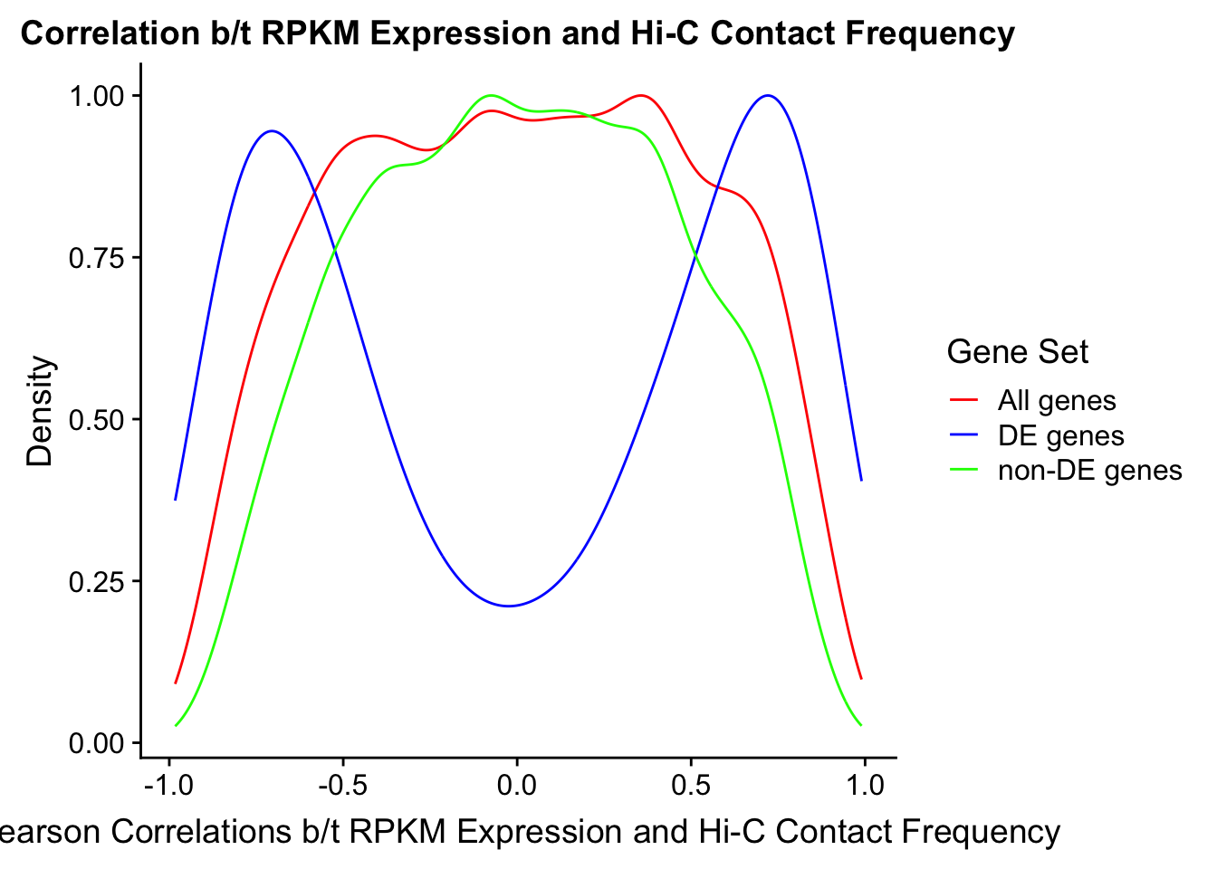
ggplot(data=ggcors) + stat_density(aes(x=cor, group=type, color=type, y=..scaled..), position="identity", geom="line") + ggtitle("Correlation b/t RPKM Expression and Hi-C Contact Frequency") + xlab("Pearson Correlations b/t RPKM Expression and Hi-C Contact Frequency") + ylab("Density") + scale_color_manual("Gene Set", values=c("red", "blue", "green", "purple", "orange", "yellow", "brown"), labels=c("All genes", "DE genes", "non-DE genes", "expression.quant1", "expression.quant2", "expression.quant3", "expression.quant4"))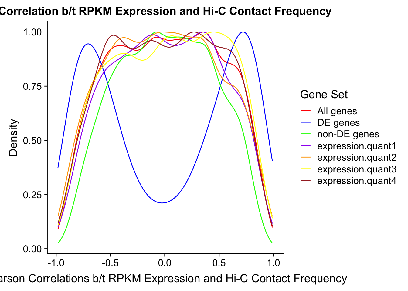
ggplot(data=filter(ggcors, type=="DE"|type=="non-DE")) + stat_density(aes(x=cor, group=type, color=type, y=..scaled..), position="identity", geom="line") + ggtitle("Correlations between Expression and Hi-C Contact Frequency") + xlab("Pearson Correlations, Expression and Hi-C Contact Frequency") + ylab("Density") + scale_color_manual("Gene Set", values=c("red", "blue"), labels=c("DE genes", "non-DE genes")) + theme(plot.title=element_text(hjust=0.2))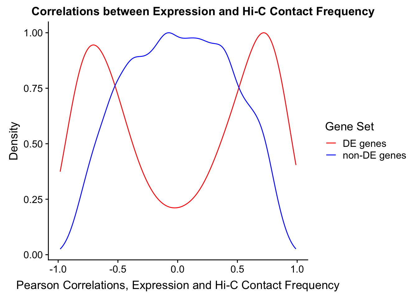
###This looks great, showing strong bimodal distribution for the DE genes and broader distributions with a peak at 0 for the non-DE set and the full set. Also see no difference in terms of the distribution of correlations on individual sets of genes stratified by quantiles of expression (mean b/t species). Note that I've done that on just DE genes as well and see slightly shorter peaks on the bimodality for the middle quantiles of expression, which makes sense (extreme unlikely to be as severe b/t species). Also, to assess if this is legit at all, I now re-run this correlation analysis after permuting the Hi-C values. I shuffle sample IDs on a gene-by-gene basis to accomplish this:
cor.permuter <- function(hicdata, exprdata, nperm){
  result <- data.frame(cor=NA, type=rep(1:nperm, each=nrow(exprdata)))
  for(perm in 1:nperm){
    permute <- hicdata
    for(row in 1:nrow(hicdata)){
      permute[row,] <- sample(hicdata[row,])
    }
    myindices <- which(result$type==perm)
    result[myindices,1] <- cor.calc(permute, exprdata)
  }
  return(result)
}

#Just do it with 10 permutations to see the general effect quickly:
full.perm <- cor.permuter(mycontacts, myexprs, 10)
DE.perm <-  cor.permuter(DEcontacts, DEexprs, 10)
nonDE.perm <- cor.permuter(nonDEcontacts, nonDEexprs, 10)

#Now visualize.
#FIGS4
ggplot(data=filter(ggcors, type=="all"|type=="DE"|type=="non-DE")) + stat_density(aes(x=cor, group=type, color=type, y=..scaled..), position="identity", geom="line") + stat_density(data=full.perm, aes(x=cor, group=type), geom="line", linetype="dotted", position="identity") + stat_density(data=DE.perm, aes(x=cor, group=type), geom="line", linetype="dashed", position="identity") + stat_density(data=nonDE.perm, aes(x=cor, group=type), geom="line", linetype="twodash", position="identity") + ggtitle("Correlation b/t RPKM Expression and Hi-C Contact Frequency") + xlab("Pearson Correlations, RPKM Expression & Hi-C Contact Frequency") + ylab("Density") + scale_color_manual("Gene Set", values=c("red", "blue", "green"), labels=c("All genes", "DE genes", "non-DE genes")) #FIGS4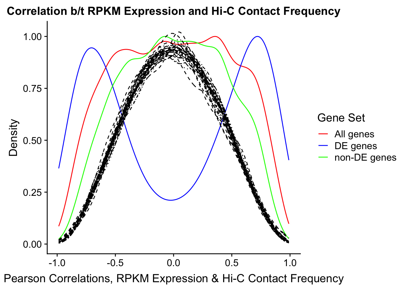
#See that permuted datasets have a tighter correlation distribution with a strong peak at 0. Reassuring. In the future I will repeat this analysis on Midway2, running 10000 permutations to see the full range of permuted data possible.

####Deprecated, for use in species-specific analysis.
# plotfull <- data.frame(fullcors=fullcors, Hcors=humcors, Ccors=chimpcors)
# plotDE <- data.frame(fullcors=fullDEcors[,1], Hcors=humDEcors[,1], Ccors=chimpDEcors[,1])
#
# ggplot(data=plotfull) + stat_density(aes(x=fullcors), geom="line") + xlab("Pearson Correlations b/t RPKM Expression and Hi-C Contact Frequency") + ylab("Density") + ggtitle("Correlations between Hi-C and Expression, all genes")
# ggplot(data=plotfull) + stat_density(aes(x=Hcors), geom="line") + xlab("Pearson Correlations b/t RPKM Expression and Hi-C Contact Frequency") + ylab("Density") + ggtitle("Correlations between Hi-C and Expression, all genes, Humans")
# ggplot(data=plotfull) + stat_density(aes(x=Ccors), geom="line") + xlab("Pearson Correlations b/t RPKM Expression and Hi-C Contact Frequency") + ylab("Density") + ggtitle("Correlations between Hi-C and Expression, all genes, Chimps")
#
# ggplot(data=plotDE) + stat_density(aes(x=fullcors), geom="line") + xlab("Pearson Correlations b/t RPKM Expression and Hi-C Contact Frequency") + ylab("Density") + ggtitle("Correlations between Hi-C and Expression, DE genes")
# ggplot(data=plotDE) + stat_density(aes(x=Hcors), geom="line") + xlab("Pearson Correlations b/t RPKM Expression and Hi-C Contact Frequency") + ylab("Density") + ggtitle("Correlations between Hi-C and Expression, DE genes, Humans")
# ggplot(data=plotDE) + stat_density(aes(x=Ccors), geom="line") + xlab("Pearson Correlations b/t RPKM Expression and Hi-C Contact Frequency") + ylab("Density") + ggtitle("Correlations between Hi-C and Expression, DE genes, Chimps")
Now that I’ve seen some nice effects in the correlation between expression and contact for different sets of genes, and for permutations on those sets, I move to see what kind of quantitiative explanatory power differential contact (DC) might actually have for differential expression (DE).
How well does Hi-C data explain expression data?
In this next section I “regress out” the effect of Hi-C contacts from their overlapping genes’ RPKM expression values, comparing a linear model run on the base values to one run on the residuals of expression after regressing out Hi-C data. Comparing the p-values before and after this regression can give some sense of whether the DE is being driven by differential Hi-C contacts (DC).
###A function to calculate gene-wise correlations between Hi-C data and expression data, but for spearman correlations. Pearson correlation calculator function is in the chunk above.
cor.calc.spear <- function(hicdata, exprdata){
  cor.exp <- vector(length=nrow(hicdata))
  for(i in 1:nrow(hicdata)){
    cor.exp[i] <- cor(as.numeric(hicdata[i,]), as.numeric(exprdata[i,]), method="spearman")
  }
  return(cor.exp)
}

###A function to permute a Hi-C df by going gene-by-gene (row-by-row) and shuffling all sample IDs.
shuffler <- function(hicdata){
    for(row in 1:nrow(hicdata)){
      hicdata[row,] <- sample(hicdata[row,])
    }
    return(hicdata)
}

###A function that runs a linear model, both with and without Hi-C corrected expression values, and returns a dataframe of hit classes (DE or not before and after correction). Also spits back out p-values before and after correction, as well as correlations between Hi-C data and expression data. Since the former is a one-row data frame of 4 points and the latter is a 3-column data frame with the number of genes rows, returns a list.
lmcorrect <- function(voom.obj, exprs, cov_matrix, meta_df){
  mygenes <- cov_matrix$genes #Pull out the relevant genes here; used for subsetting the voom.obj in a bit.
  cov_matrix <- cov_matrix[, -9] #Remove genes from the cov matrix
  hic_present <- sapply(1:nrow(cov_matrix), function(i) !any(is.na(cov_matrix[i,]))) #First, remove any rows w/ missing Hi-C data.
  exprs <- data.matrix(exprs[hic_present,]) #Filter expression with this
  cov_matrix <- data.matrix(cov_matrix[hic_present,]) #Filter Hi-C data with this

  #Now, prepare to run the actual models. First run a model w/ Hi-C as a covariate to evaluate
  SP <- factor(meta_df$SP,levels = c("H","C"))
  design <- model.matrix(~0+SP)
  colnames(design) <- c("Human", "Chimp")
  resid_hic <- array(0, dim=c(nrow(exprs), ncol(cov_matrix))) #Initialize a dataframe for storing the residuals.
  for(i in 1:nrow(exprs)){#Loop through rows of the expression df, running linear modeling w/ Hi-C to obtain residuals.
   resid_hic[i,] <- lm(exprs[i,]~cov_matrix[i,])$resid
  }

  mycon <- makeContrasts(HvC = Human-Chimp, levels = design)

  #Filter the voom object to only contain genes that had Hi-C information here.
  good.indices <- which(rownames(voom.obj$E) %in% mygenes)
  voom.obj <- voom.obj[good.indices,]

  #Now, replace the RPKM values in the voom object for after linear modeling with the residuals.
  voom.obj.after <- voom.obj
  voom.obj.after$E <- resid_hic

  lmFit(voom.obj, design=design) %>% eBayes(.) %>% contrasts.fit(., mycon) %>% eBayes(.) %>% topTable(., coef = 1, adjust.method = "BH", number = Inf, sort.by="none") -> fit_before
  lmFit(voom.obj.after, design=design) %>% eBayes(.) %>% contrasts.fit(., mycon) %>% eBayes(.) %>% topTable(., coef = 1, adjust.method = "BH", number = Inf, sort.by="none") -> fit_after

  result.DE.cats <- data.frame(DEneither=sum(fit_before$adj.P.Val>0.05&fit_after$adj.P.Val>0.05), DEbefore=sum(fit_before$adj.P.Val<=0.05&fit_after$adj.P.Val>0.05), DEafter=sum(fit_before$adj.P.Val>0.05&fit_after$adj.P.Val<=0.05), DEboth=sum(fit_before$adj.P.Val<=0.05&fit_after$adj.P.Val<=0.05))
  result.DE.stats <- data.frame(cor.pear=cor.calc(cov_matrix, exprs), cor.spear=cor.calc.spear(cov_matrix, exprs), pval.before=fit_before$adj.P.Val, pval.after=fit_after$adj.P.Val)
  result <- list("categories"=result.DE.cats, "stats"=result.DE.stats)
  return(result)
}

#Proceed to use the function on the different dataframes I've created with different sets of overlapping Hi-C contacts:
h_minFDR_pvals <- lmcorrect(weighted.data, hmin[,c("A-21792", "B-28126", "C-3649", "D-40300", "E-28815", "F-28834", "G-3624", "H-3651")], hmin[,c("A_21792_HIC", "B_28126_HIC", "C_3649_HIC", "D_40300_HIC", "E_28815_HIC", "F_28834_HIC", "G_3624_HIC", "H_3651_HIC", "genes")], meta.data)
c_minFDR_pvals <- lmcorrect(weighted.data, cmin[,c("A-21792", "B-28126", "C-3649", "D-40300", "E-28815", "F-28834", "G-3624", "H-3651")], cmin[,c("A_21792_HIC", "B_28126_HIC", "C_3649_HIC", "D_40300_HIC", "E_28815_HIC", "F_28834_HIC", "G_3624_HIC", "H_3651_HIC", "genes")], meta.data)
h_maxB_pvals <- lmcorrect(weighted.data, hmaxB[,c("A-21792", "B-28126", "C-3649", "D-40300", "E-28815", "F-28834", "G-3624", "H-3651")], hmaxB[,c("A_21792_HIC", "B_28126_HIC", "C_3649_HIC", "D_40300_HIC", "E_28815_HIC", "F_28834_HIC", "G_3624_HIC", "H_3651_HIC", "genes")], meta.data)
c_maxB_pvals <- lmcorrect(weighted.data, cmaxB[,c("A-21792", "B-28126", "C-3649", "D-40300", "E-28815", "F-28834", "G-3624", "H-3651")], cmaxB[,c("A_21792_HIC", "B_28126_HIC", "C_3649_HIC", "D_40300_HIC", "E_28815_HIC", "F_28834_HIC", "G_3624_HIC", "H_3651_HIC", "genes")], meta.data)
h_US_pvals <- lmcorrect(weighted.data, hUS[,c("A-21792", "B-28126", "C-3649", "D-40300", "E-28815", "F-28834", "G-3624", "H-3651")], hUS[,c("A_21792_HIC", "B_28126_HIC", "C_3649_HIC", "D_40300_HIC", "E_28815_HIC", "F_28834_HIC", "G_3624_HIC", "H_3651_HIC", "genes")], meta.data)
c_US_pvals <- lmcorrect(weighted.data, cUS[,c("A-21792", "B-28126", "C-3649", "D-40300", "E-28815", "F-28834", "G-3624", "H-3651")], cUS[,c("A_21792_HIC", "B_28126_HIC", "C_3649_HIC", "D_40300_HIC", "E_28815_HIC", "F_28834_HIC", "G_3624_HIC", "H_3651_HIC", "genes")], meta.data)

#I now proceed to visualize the difference in p-values for expression before and after "correcting" for the Hi-C data. I am hoping to see many hits in the bottom right quadrant of the following plots, indicating genes that showed up as DE before Hi-C correction, but not after. I also expect that p-values falling farther away from the null line of expectation for p-values being identical between models will have higher correlations, which I color here for the pearson correlation (results look similar for spearman).
ggplot(data=h_minFDR_pvals$stats, aes(x=-log10(pval.before), y=-log10(pval.after), color=abs(cor.pear))) + geom_point(size=0.01) + geom_hline(yintercept=-log10(0.05), color="red") + geom_vline(xintercept=-log10(0.05), color="red") + geom_abline(slope=1, intercept=0, color="green", linetype="dashed") + ggtitle("Evidence for DE before vs. after regressing out Hi-C contact frequency") + xlab("-log10(p-value of DE before Hi-C regression)") + ylab("-log10(p-value of DE after Hi-C regression")
ggplot(data=h_minFDR_pvals$stats, aes(x=-log10(pval.before), y=-log10(pval.after))) + geom_point(size=0.01) + geom_hline(yintercept=-log10(0.05), color="red") + geom_vline(xintercept=-log10(0.05), color="red") + geom_abline(slope=1, intercept=0, color="green", linetype="dashed") + ggtitle("Evidence for DE Before vs. After Regressing out Hi-C Contact Frequency") + xlab("-log10(p-value of DE before Hi-C regression)") + ylab("-log10(p-value of DE after Hi-C regression)") + theme(plot.title=element_text(hjust=1)) #Slightly cleaner, for MindBytes 2018 posterggplot(data=h_maxB_pvals$stats, aes(x=-log10(pval.before), y=-log10(pval.after), color=abs(cor.pear))) + geom_point(size=0.01) + geom_hline(yintercept=-log10(0.05), color="red") + geom_vline(xintercept=-log10(0.05), color="red") + geom_abline(slope=1, intercept=0, color="green", linetype="dashed") + ggtitle("Evidence for DE before vs. after regressing out Hi-C max beta (H)") + xlab("-log10(p-value of DE before Hi-C regression)") + ylab("-log10(p-value of DE after Hi-C regression")ggplot(data=h_US_pvals$stats, aes(x=-log10(pval.before), y=-log10(pval.after), color=abs(cor.spear))) + geom_point(size=0.01) + geom_hline(yintercept=-log10(0.05), color="red") + geom_vline(xintercept=-log10(0.05), color="red") + geom_abline(slope=1, intercept=0, color="green", linetype="dashed") + ggtitle("Evidence for DE before vs. after regressing out Hi-C US bin FDR (H)") + xlab("-log10(p-value of DE before Hi-C regression)") + ylab("-log10(p-value of DE after Hi-C regression")ggplot(data=c_minFDR_pvals$stats, aes(x=-log10(pval.before), y=-log10(pval.after), color=abs(cor.pear))) + geom_point(size=0.01) + geom_hline(yintercept=-log10(0.05), color="red") + geom_vline(xintercept=-log10(0.05), color="red") + geom_abline(slope=1, intercept=0, color="green", linetype="dashed") + ggtitle("Evidence for DE before vs. after regressing out Hi-C min. FDR (C)") + xlab("-log10(p-value of DE before Hi-C regression)") + ylab("-log10(p-value of DE after Hi-C regression")ggplot(data=c_maxB_pvals$stats, aes(x=-log10(pval.before), y=-log10(pval.after), color=abs(cor.pear))) + geom_point(size=0.01) + geom_hline(yintercept=-log10(0.05), color="red") + geom_vline(xintercept=-log10(0.05), color="red") + geom_abline(slope=1, intercept=0, color="green", linetype="dashed") + ggtitle("Evidence for DE before vs. after regressing out Hi-C max beta (C)") + xlab("-log10(p-value of DE before Hi-C regression)") + ylab("-log10(p-value of DE after Hi-C regression")ggplot(data=c_US_pvals$stats, aes(x=-log10(pval.before), y=-log10(pval.after), color=abs(cor.pear))) + geom_point(size=0.01) + geom_hline(yintercept=-log10(0.05), color="red") + geom_vline(xintercept=-log10(0.05), color="red") + geom_abline(slope=1, intercept=0, color="green", linetype="dashed") + ggtitle("Evidence for DE before vs. after regressing out Hi-C US bin FDR (C)") + xlab("-log10(p-value of DE before Hi-C regression)") + ylab("-log10(p-value of DE after Hi-C regression") Critically, here I see that “regressing out” Hi-C data and trying to model expression again moves many genes from being significantly differentially expressed (at FDR of 5%) to no longer showing differential expression. Seeing most of the hits in the bottom right corner of these visualizations is what confirms this. Reassuringly, I also see stronger correlations between RPKM expression values and normalized Hi-C interaction frequency values for points farther away from the diagonal green line of expectation. However, since this is not a statistical test, I have no assessment of significance. To accomplish this, I compare these results to running the same kind of analysis on permuted data in the next section.
Permutation Visualizations
Here, I visualize the difference in classes of DE hits changing (either gaining, losing, or maintaining DE status) after “regressing out” the effect of Hi-C from expression. I show distributions of these percentages across 10000 permutations of the data, as compared to the observed percentages.
##Visualization of the permutations!
perm.vis <- function(categories.df.file, df, metadata, hictype, DE=FALSE){
  if(DE==TRUE){expected1 <- readRDS(paste("~/Desktop/Hi-C/HiC_covs/results/new_results/DE/batch1/", categories.df.file, sep=""))
  expected2 <-  readRDS(paste("~/Desktop/Hi-C/HiC_covs/results/new_results/DE/batch2/", categories.df.file, sep=""))
  observed <- lmcorrect(weighted.data, df[which(df$adj.P.Val<=0.05), c("A-21792", "B-28126", "C-3649", "D-40300", "E-28815", "F-28834", "G-3624", "H-3651")], df[which(df$adj.P.Val<=0.05), c("A_21792_HIC", "B_28126_HIC", "C_3649_HIC", "D_40300_HIC", "E_28815_HIC", "F_28834_HIC", "G_3624_HIC", "H_3651_HIC", "genes")], metadata)
  }
  else{expected1 <- readRDS(paste("~/Desktop/Hi-C/HiC_covs/results/new_results/batch1/", categories.df.file, sep=""))
  expected2 <- readRDS(paste("~/Desktop/Hi-C/HiC_covs/results/new_results/batch2/", categories.df.file, sep=""))
  observed <- lmcorrect(weighted.data, df[,c("A-21792", "B-28126", "C-3649", "D-40300", "E-28815", "F-28834", "G-3624", "H-3651")], df[,c("A_21792_HIC", "B_28126_HIC", "C_3649_HIC", "D_40300_HIC", "E_28815_HIC", "F_28834_HIC", "G_3624_HIC", "H_3651_HIC", "genes")], metadata)
  }
  expected <- c(expected1[1:5000], expected2[1:5000])
  expected[[10001]] <- rbind(expected1[[5001]], expected2[[5001]])
  expected[[10001]] <- ((expected[[10001]])/sum(expected[[10001]][1,]))*100
  for(i in 1:(length(expected)-1)){
  expected[[i]]$type <- i
  expected[[i]]$data <- "expected"
  }
  observed$categories <- (observed$categories/sum(observed$categories[1,]))*100
  observed$stats$type <- 10001
  observed$stats$data <- "observed"
  expected[[10001]]$data <- "permutations"
  expected[[10001]][10001,] <- c(observed$categories, "observation")
  deneitherbox <- ggplot(data=expected[[10001]], aes(x="", y=DEneither)) + geom_boxplot(aes(color="Expected"), show.legend=FALSE) + geom_point(aes(y=observed$categories$DEneither, color="Observed"), size=3) + ggtitle("Percent of genes with no evidence for DE regardless") + ylab("% genes not DE in either") + xlab(paste("10000 Permutations of Hi-C data ", hictype, sep="")) + scale_color_manual(values=c("blue", "red"), guide=FALSE) +guides(color=guide_legend("Data", override.aes = list(shape=c(16, 16))))
  debeforebox <- ggplot(data=expected[[10001]], aes(x="", y=DEbefore)) + geom_boxplot(aes(color="Expected"), show.legend=FALSE) + geom_point(aes(y=observed$categories$DEbefore, color="Observed"), size=3) + ggtitle("Percent of genes with reduced evidence for DE after Hi-C correction") + ylab("% genes DE before, but not after, Hi-C correction") + xlab(paste("10000 Permutations of Hi-C data ", hictype, sep="")) + scale_color_manual(values=c("blue", "red"), guide=FALSE) +guides(color=guide_legend("Data", override.aes = list(shape=c(16, 16))))
  deafterbox <- ggplot(data=expected[[10001]], aes(x="", y=DEafter)) + geom_boxplot(aes(color="Expected"), show.legend=FALSE) + geom_point(aes(y=observed$categories$DEafter, color="Observed"), size=3) + ggtitle("Percent of genes with increased evidence for DE after Hi-C correction") + ylab("% genes DE after, but not before, Hi-C correction") + xlab(paste("10000 Permutations of Hi-C data ", hictype, sep="")) + scale_color_manual(values=c("blue", "red"), guide=FALSE) +guides(color=guide_legend("Data", override.aes = list(shape=c(16, 16))))
  debothbox <- ggplot(data=expected[[10001]], aes(x="", y=DEboth)) + geom_boxplot(aes(color="Expected"), show.legend=FALSE) + geom_point(aes(y=observed$categories$DEboth, color="Observed"), size=3) + ggtitle("Percent of genes with evidence for DE regardless") + ylab("% genes DE in both") + xlab(paste("10000 Permutations of Hi-C data ", hictype, sep="")) + scale_color_manual(values=c("blue", "red"), guide=FALSE) +guides(color=guide_legend("Data", override.aes = list(shape=c(16, 16))))
  print(deneitherbox)
  print(debeforebox)
  print(deafterbox)
  print(debothbox)
}

perm.vis("permout_h_minFDR", hmin, meta.data, "(min FDR contact, Humans)")

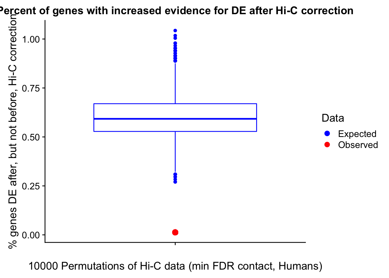

perm.vis("permout_h_maxB", hmaxB, meta.data, "(max beta contact, Humans)")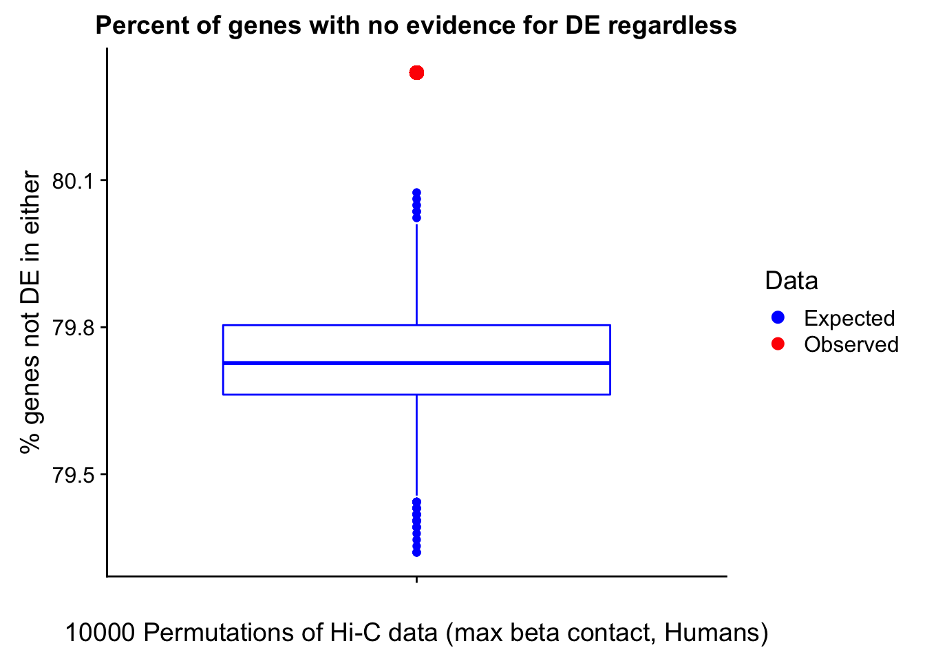

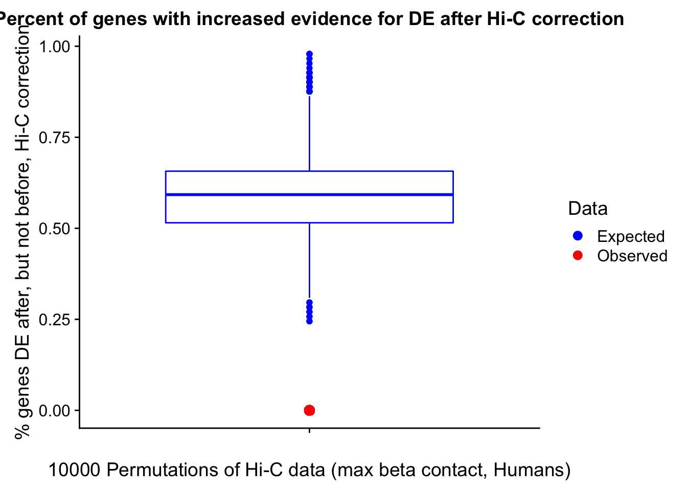
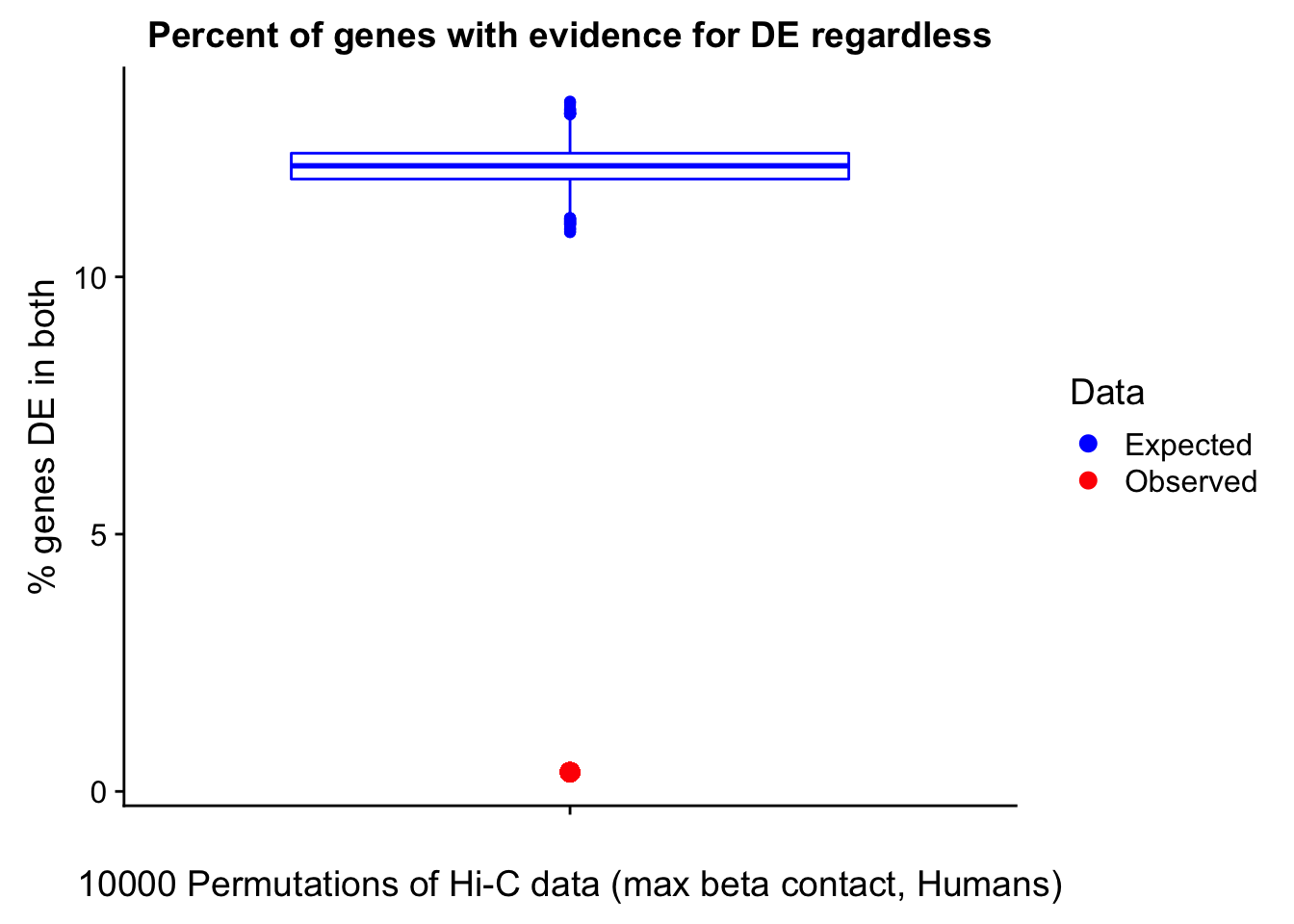
perm.vis("permout_h_US", hUS, meta.data, "(upstream contact, Humans)")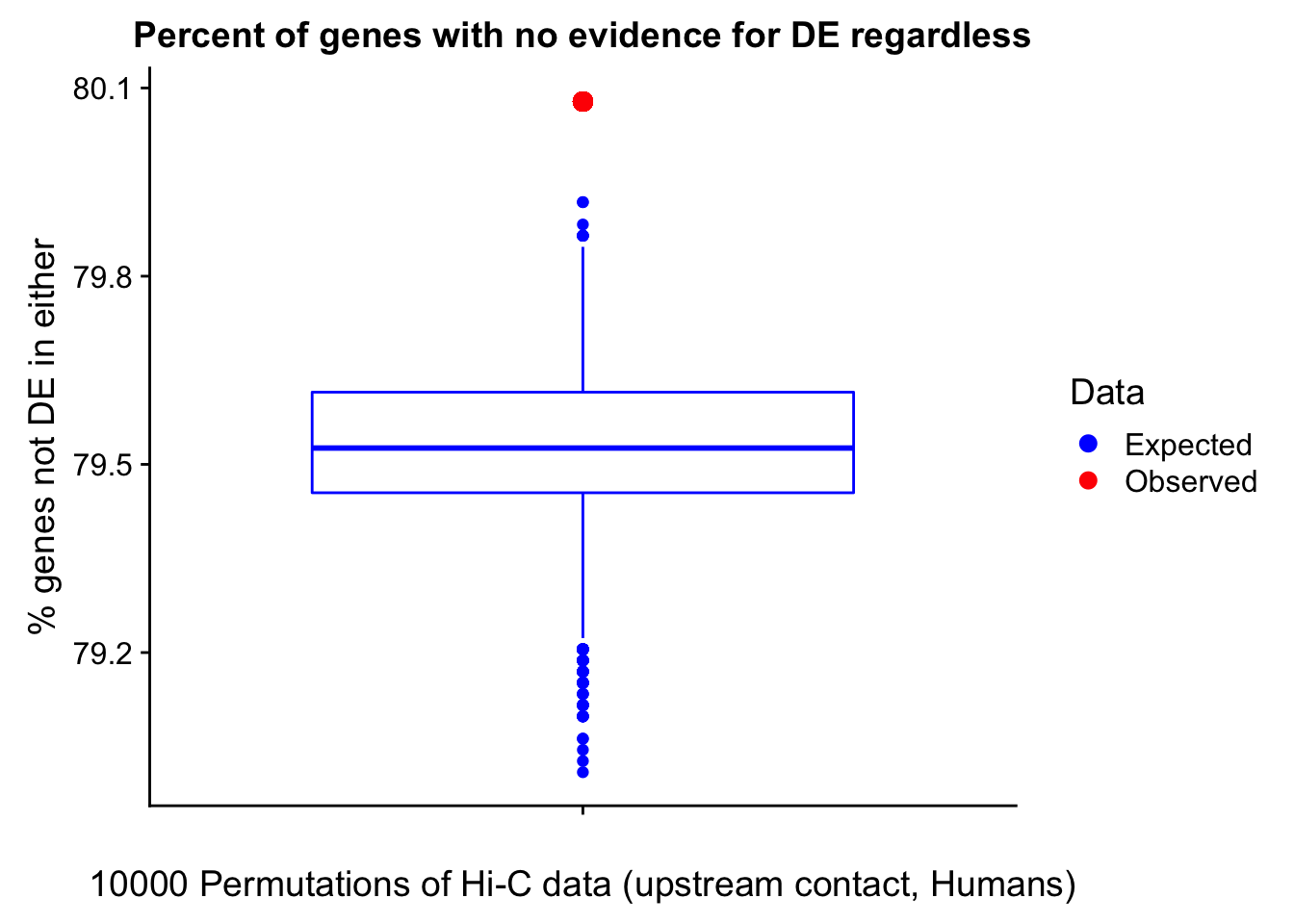
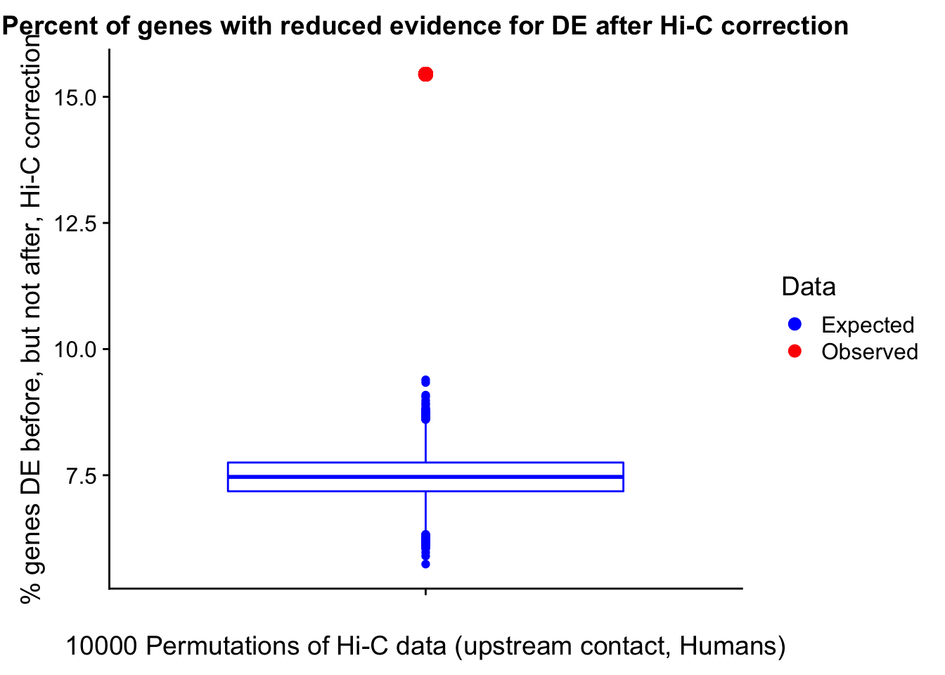
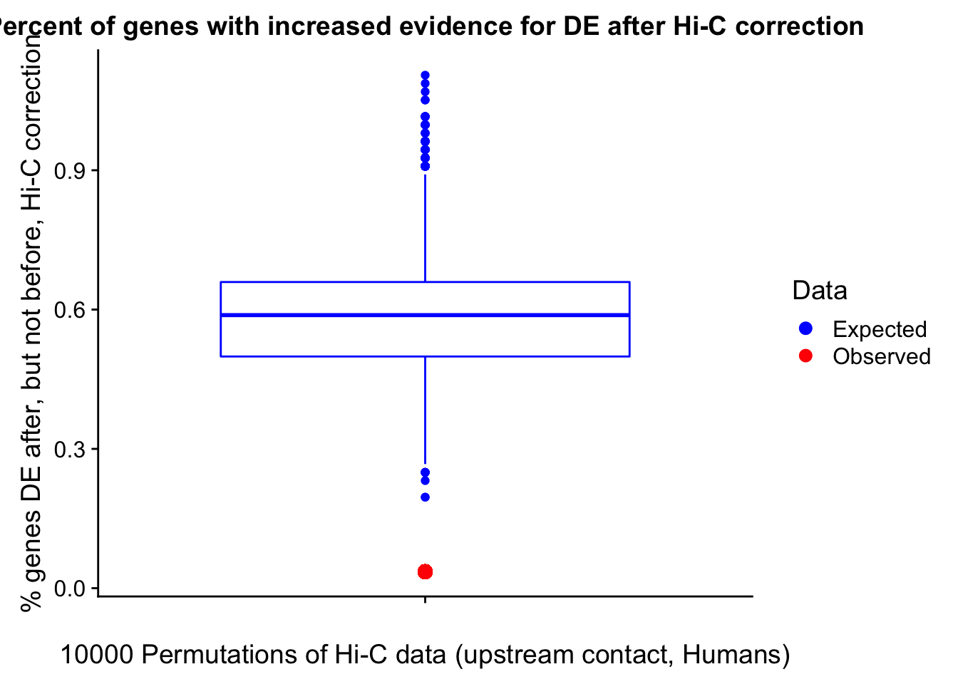
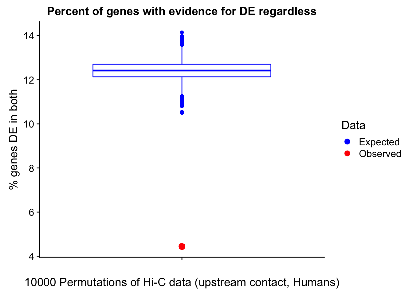
perm.vis("permout_c_minFDR", cmin, meta.data, "(min FDR contact, Chimps)")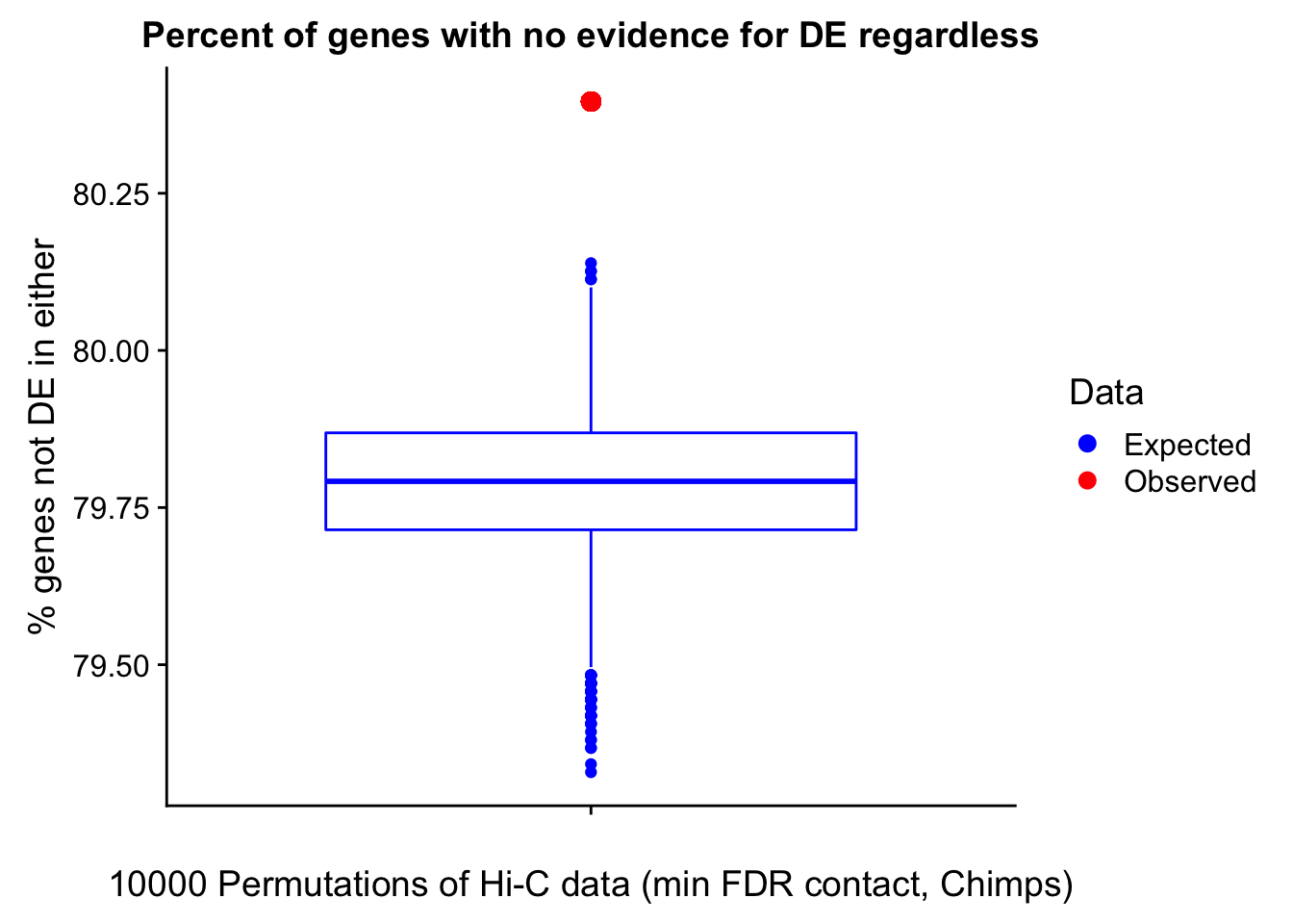
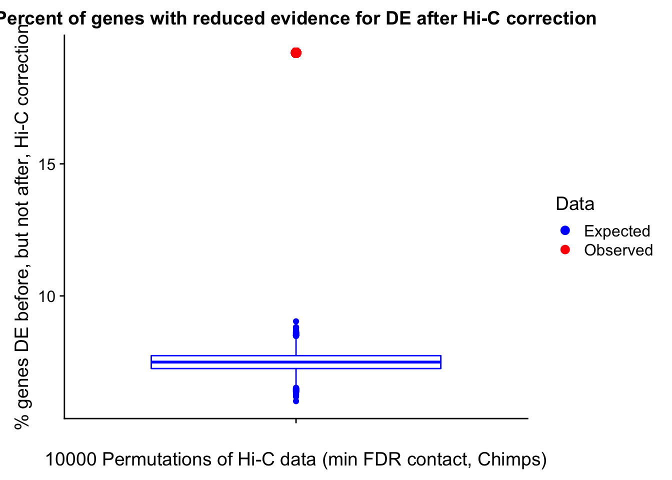
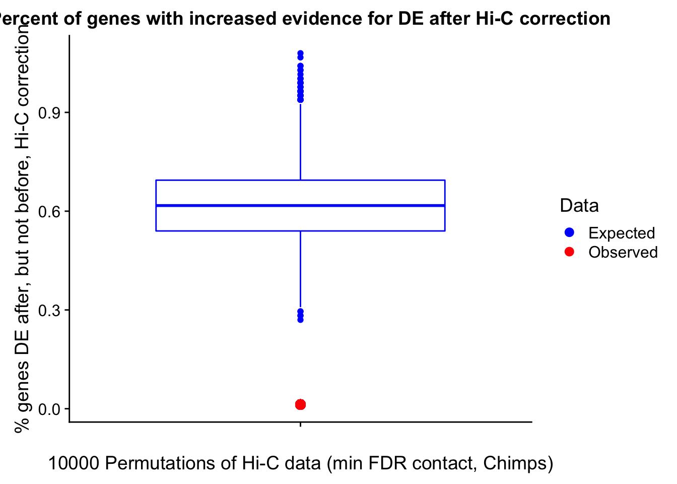
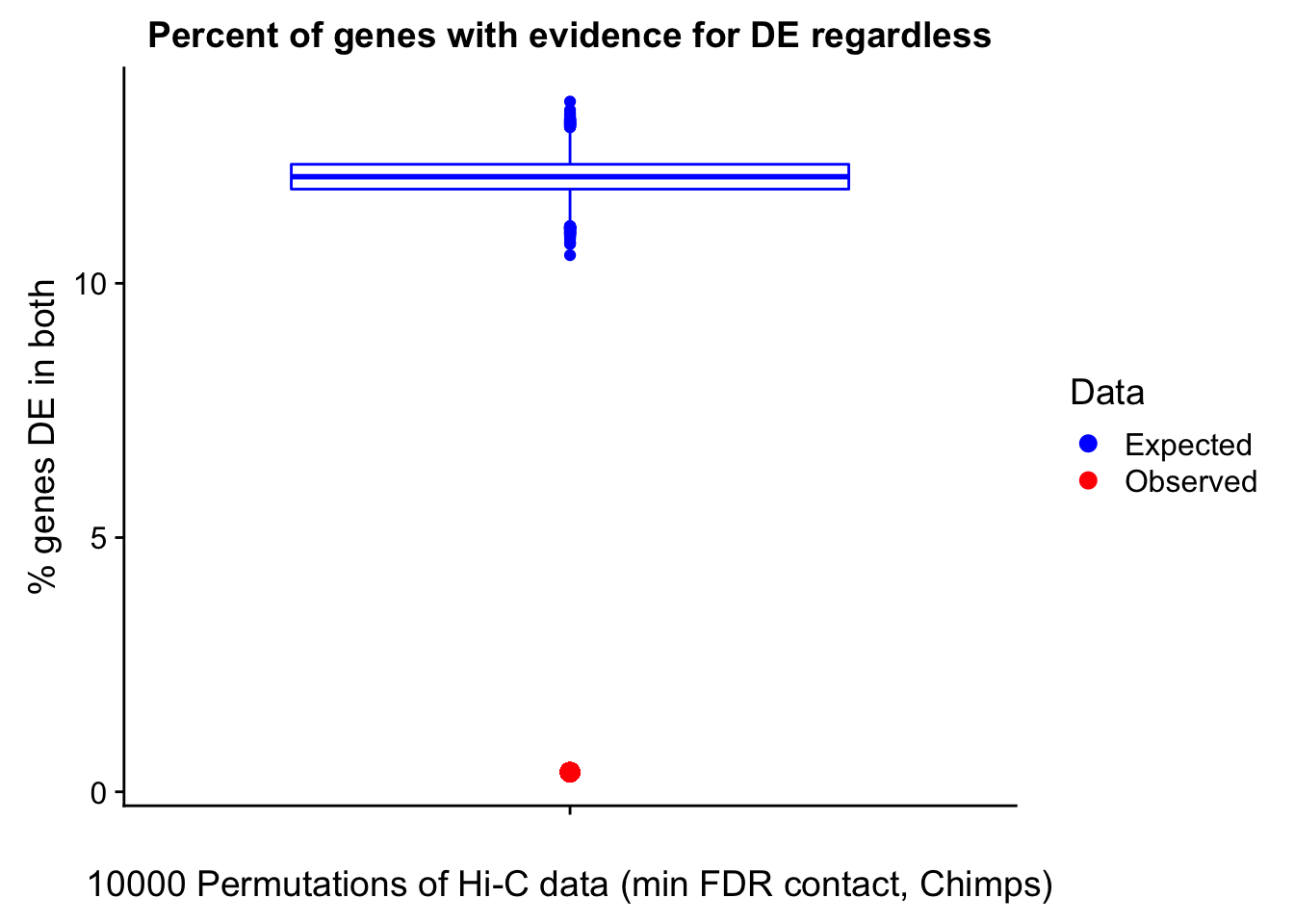
perm.vis("permout_c_maxB", cmaxB, meta.data, "(max beta contact, Chimps)")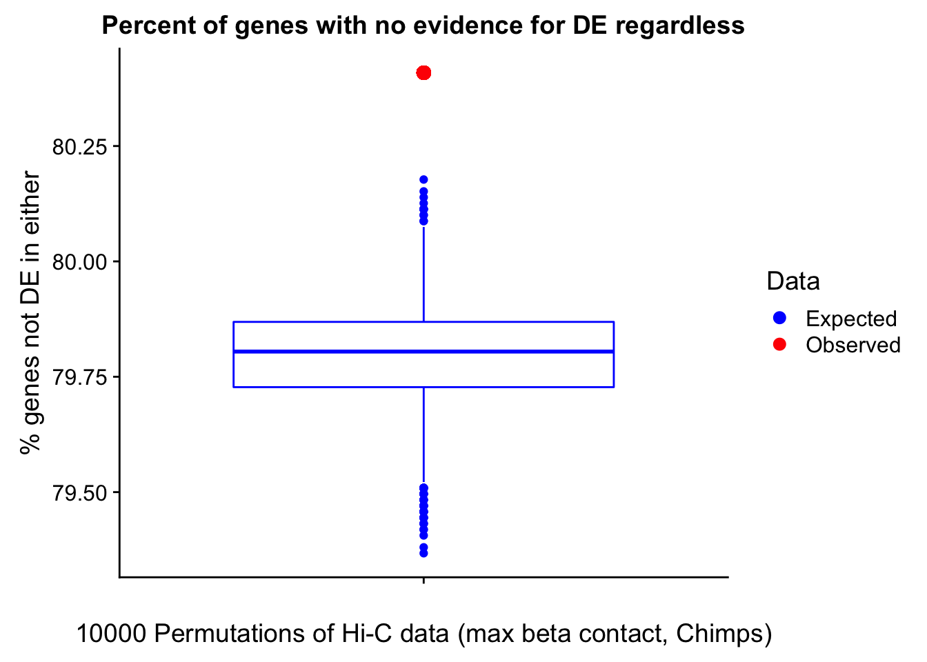

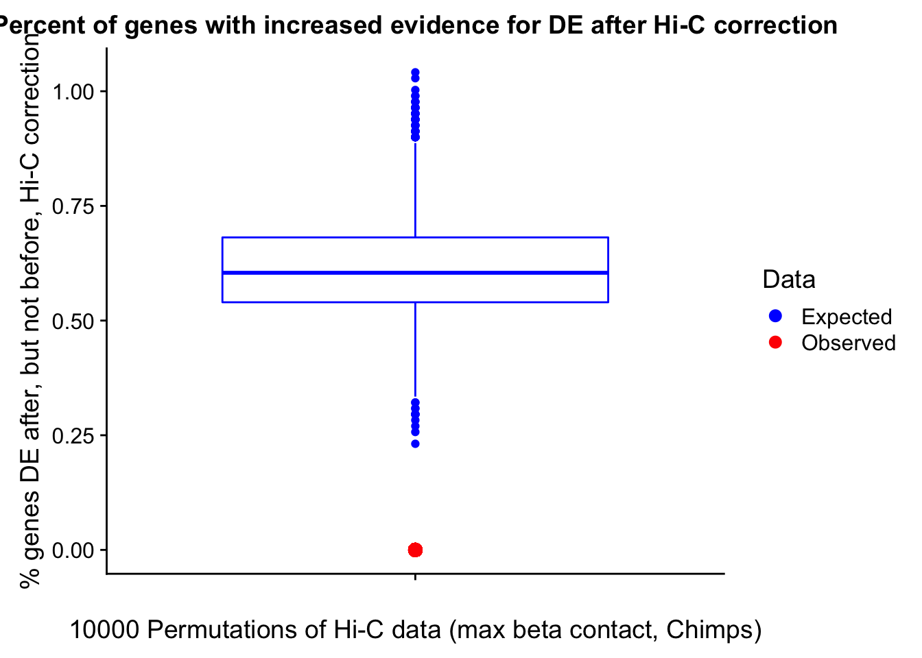
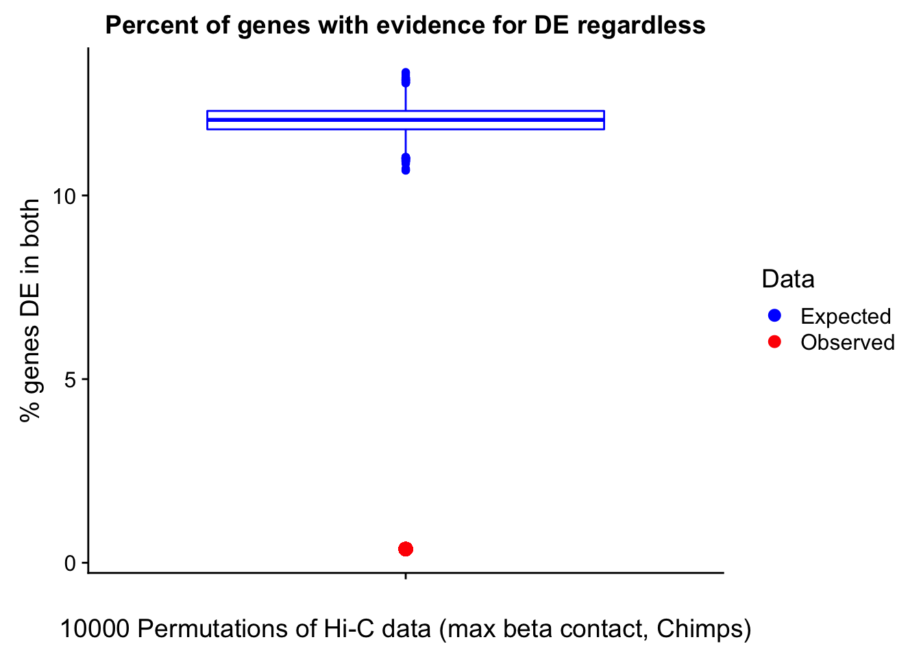
perm.vis("permout_c_US", cUS, meta.data, "(upstream contact, Chimps)")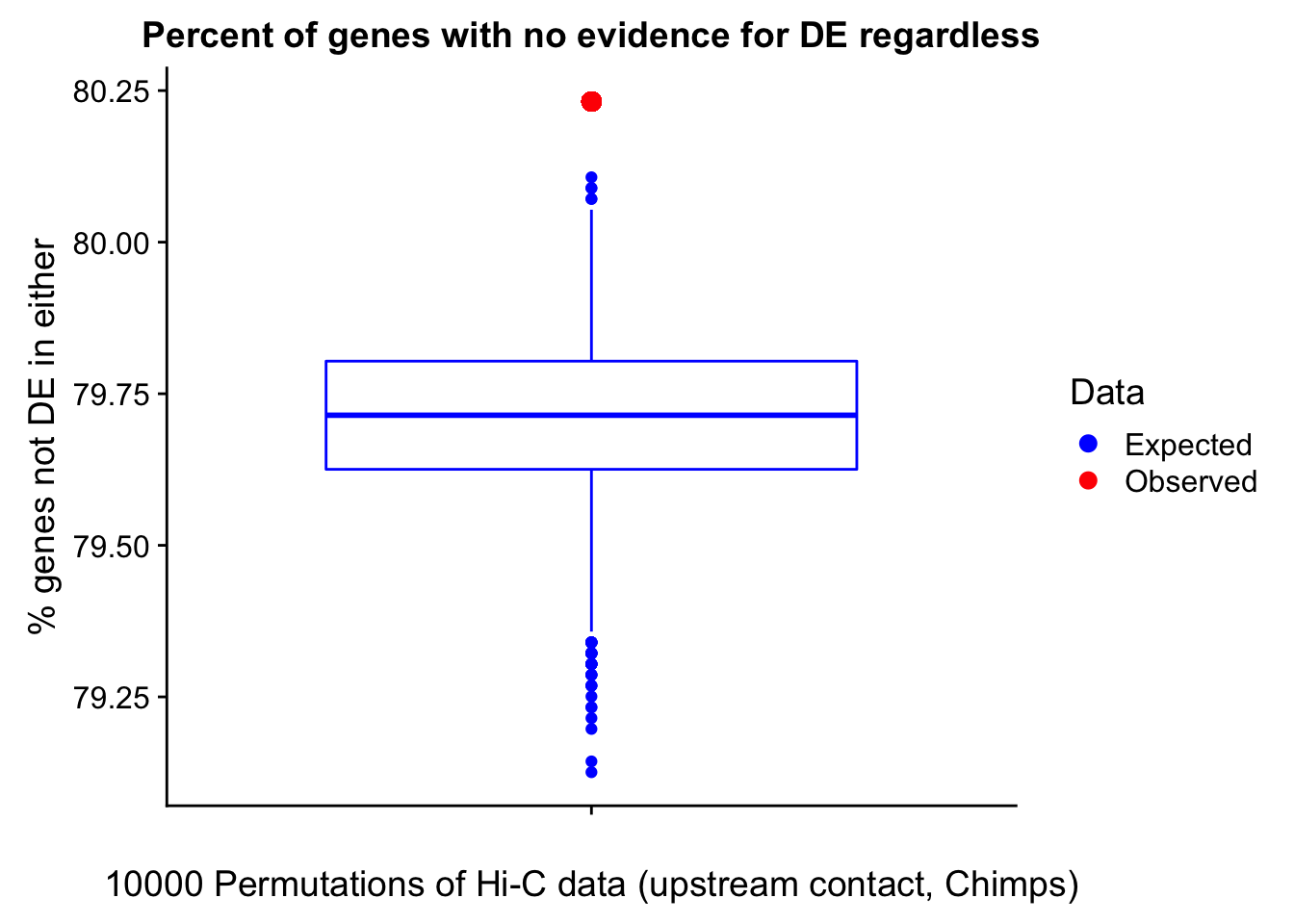
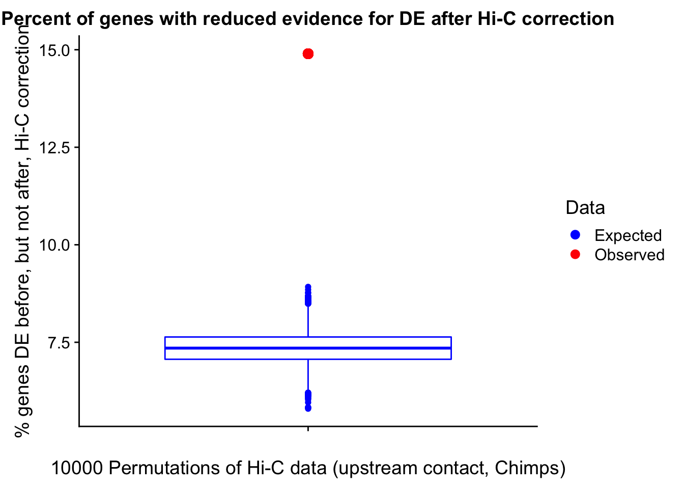
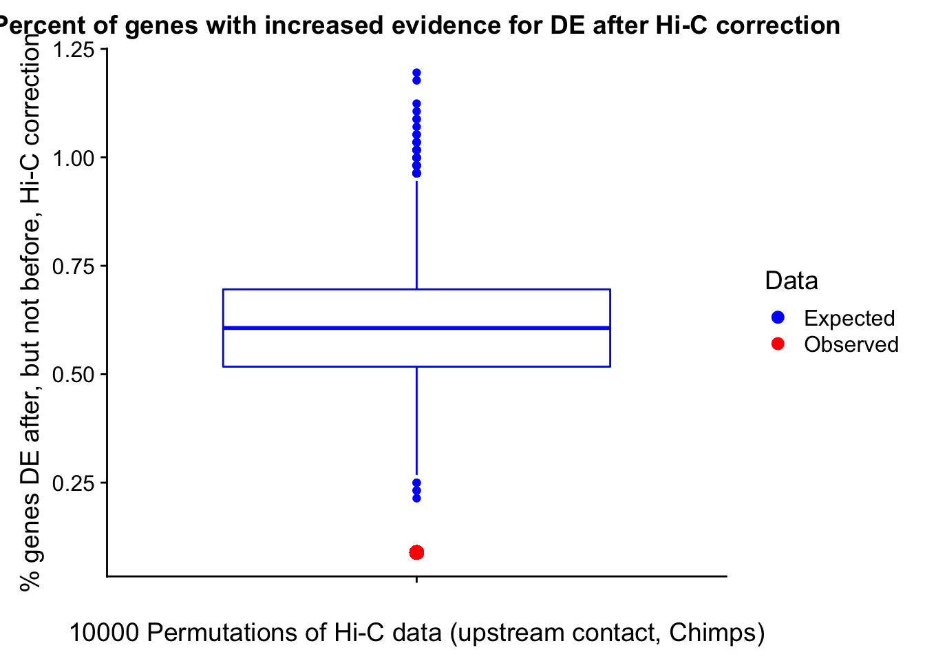

perm.vis("permout_h_minFDR_DE", hminDE, meta.data, "(min FDR contact, Humans)", DE=TRUE)
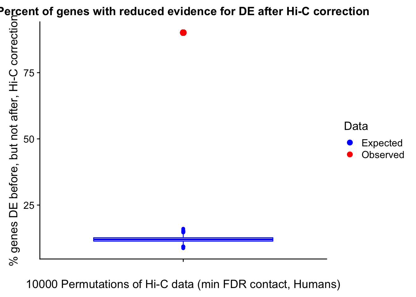

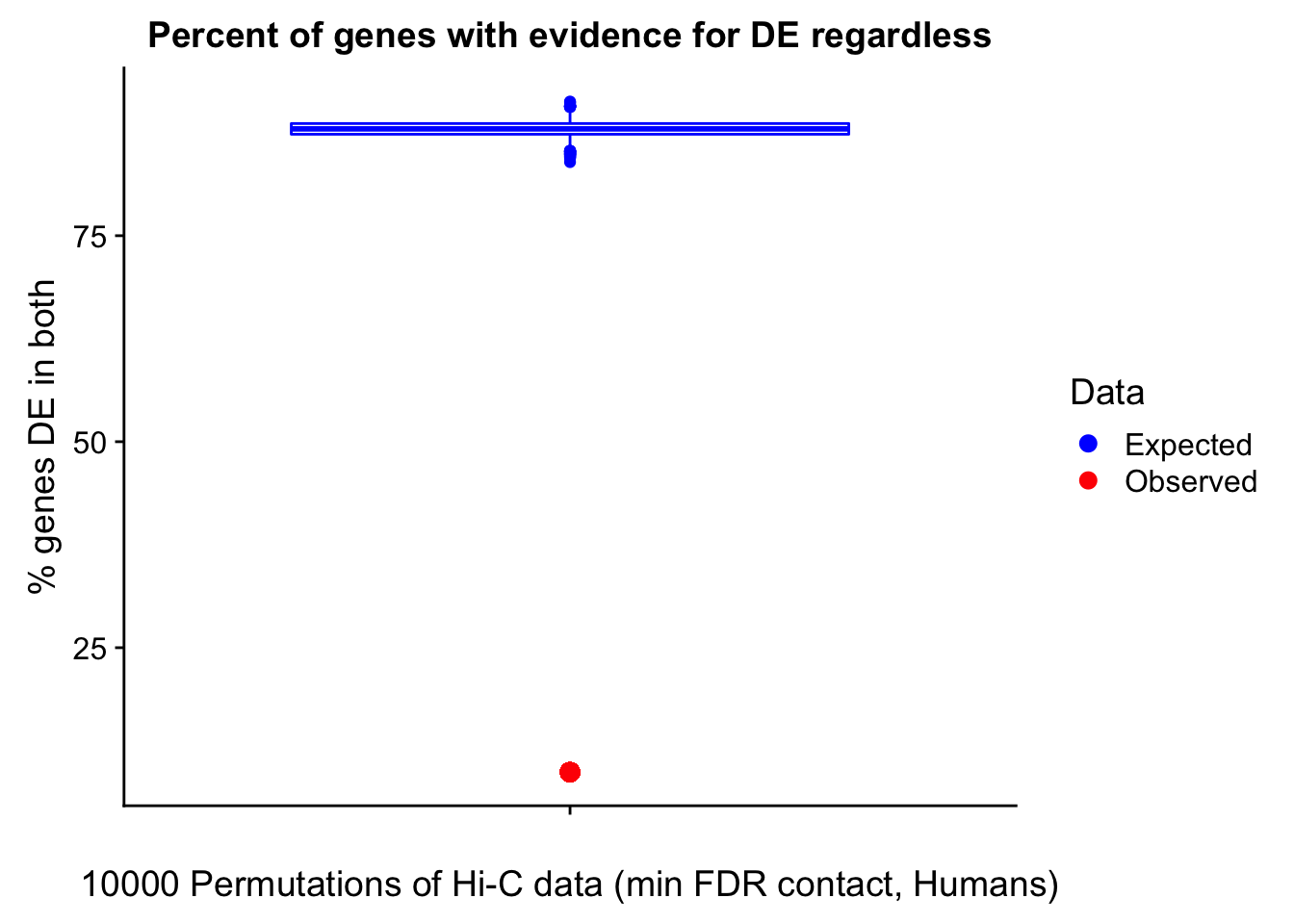
perm.vis("permout_h_maxB_DE", hmaxBDE, meta.data, "(max beta contact, Humans)", DE=TRUE)
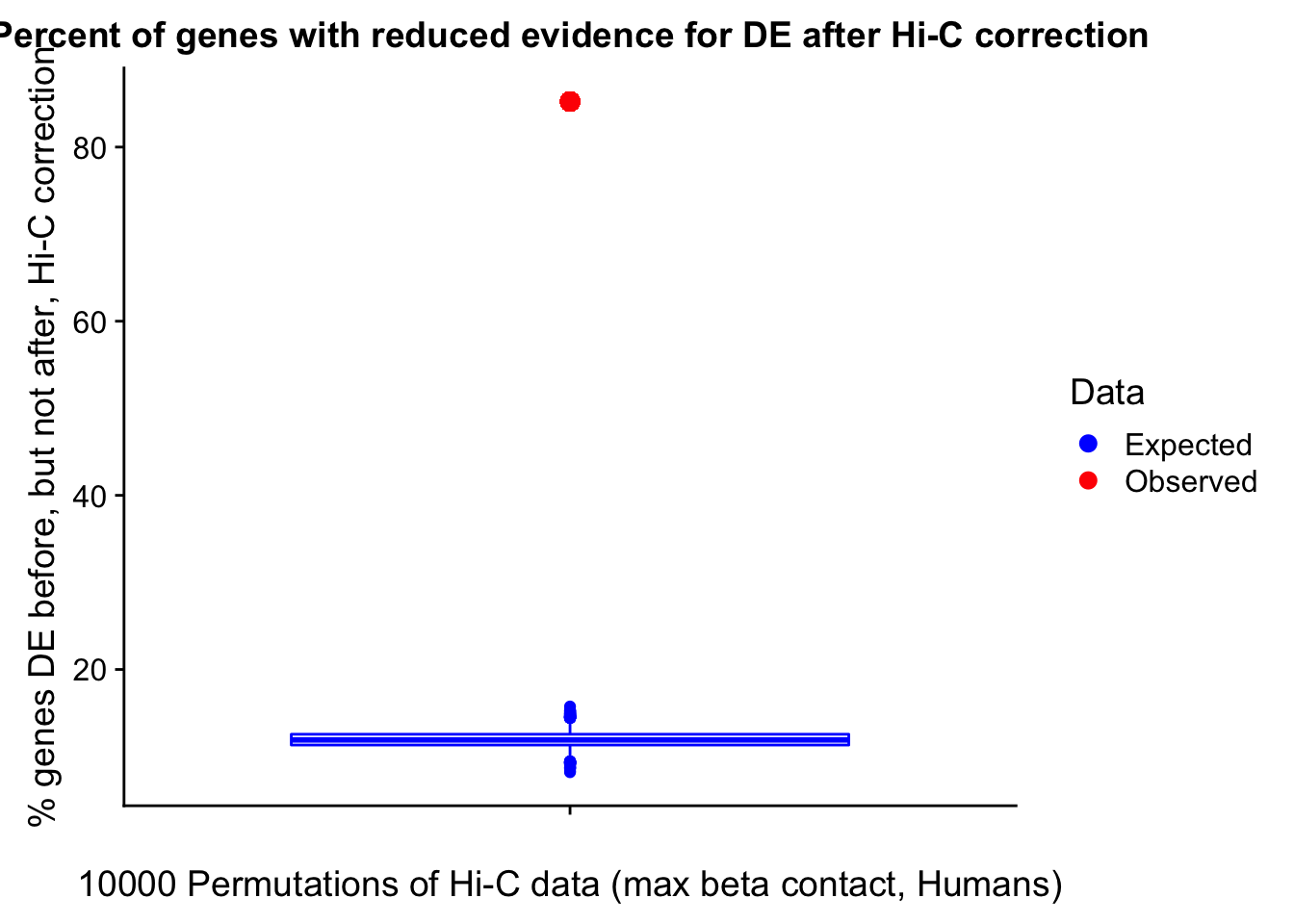
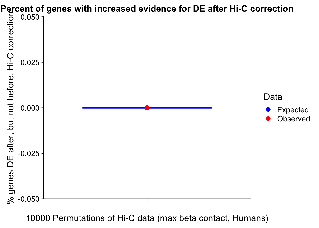
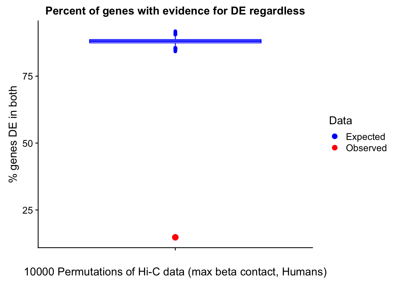
perm.vis("permout_h_US_DE", hUSDE, meta.data, "(upstream contact, Humans)", DE=TRUE)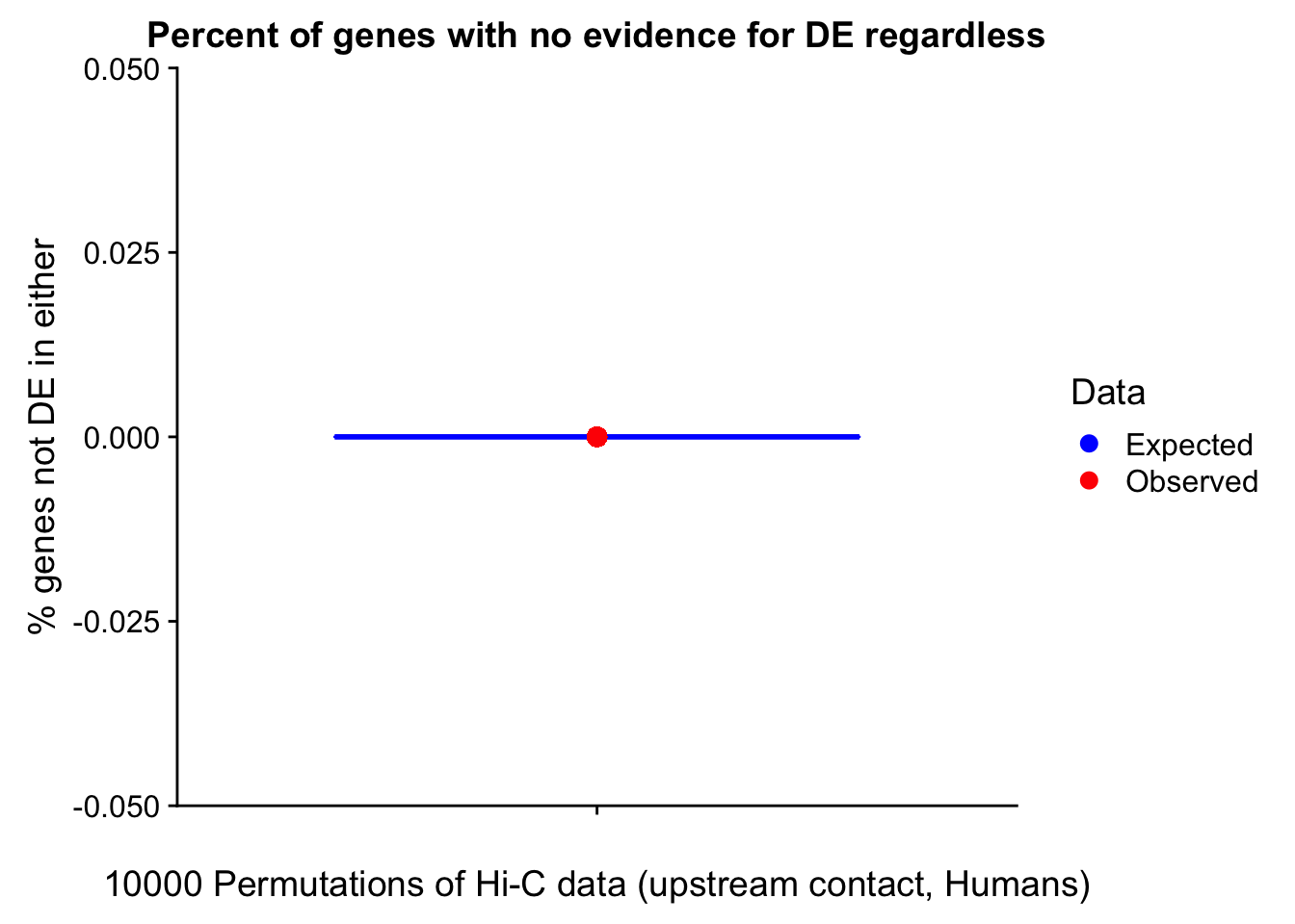
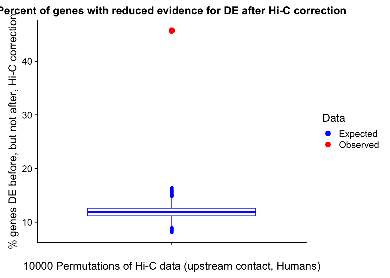

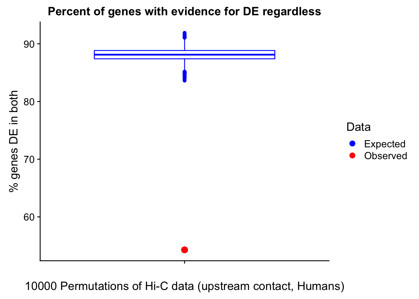
perm.vis("permout_c_minFDR_DE", cminDE, meta.data, "(min FDR contact, Chimps)", DE=TRUE)

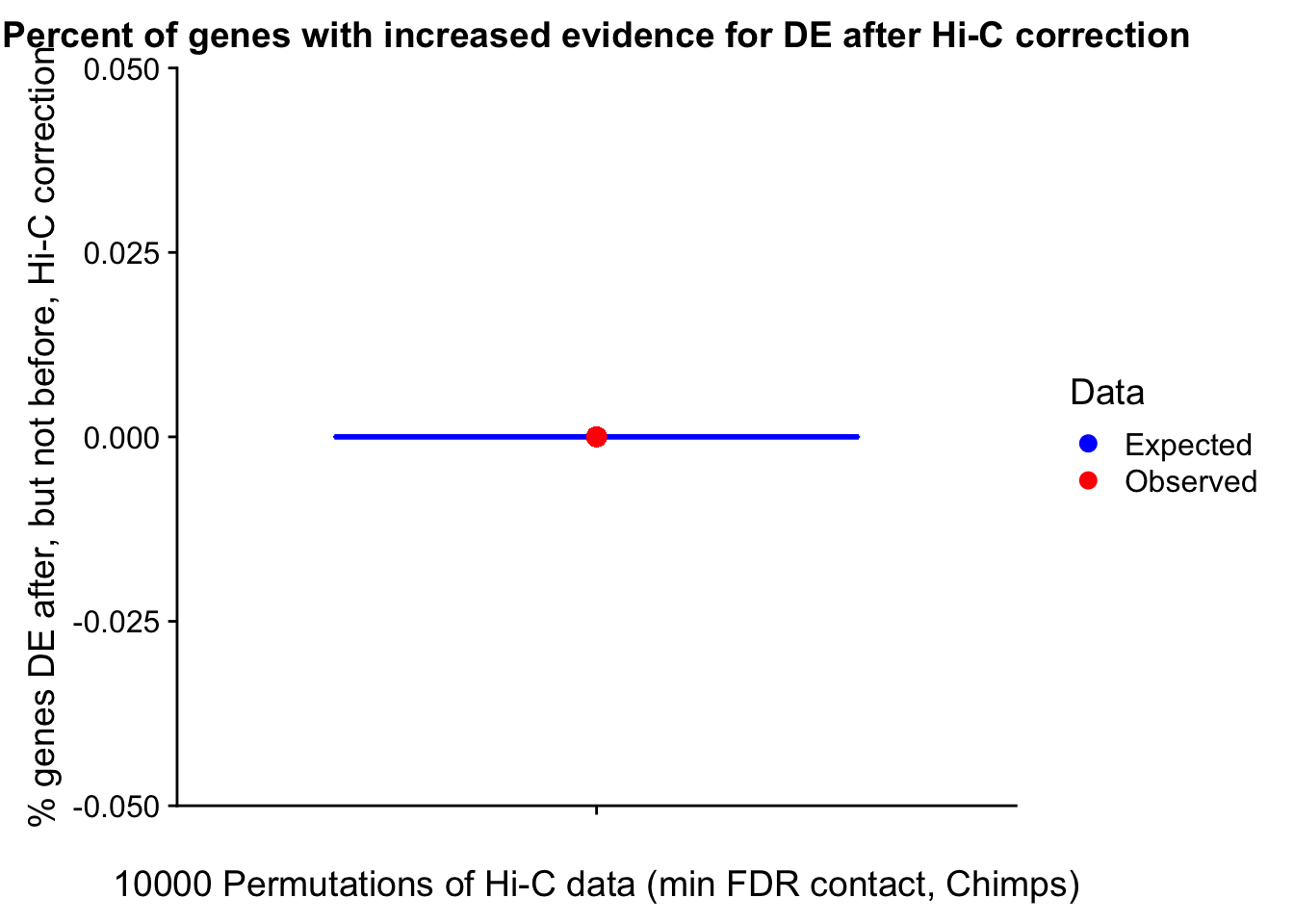
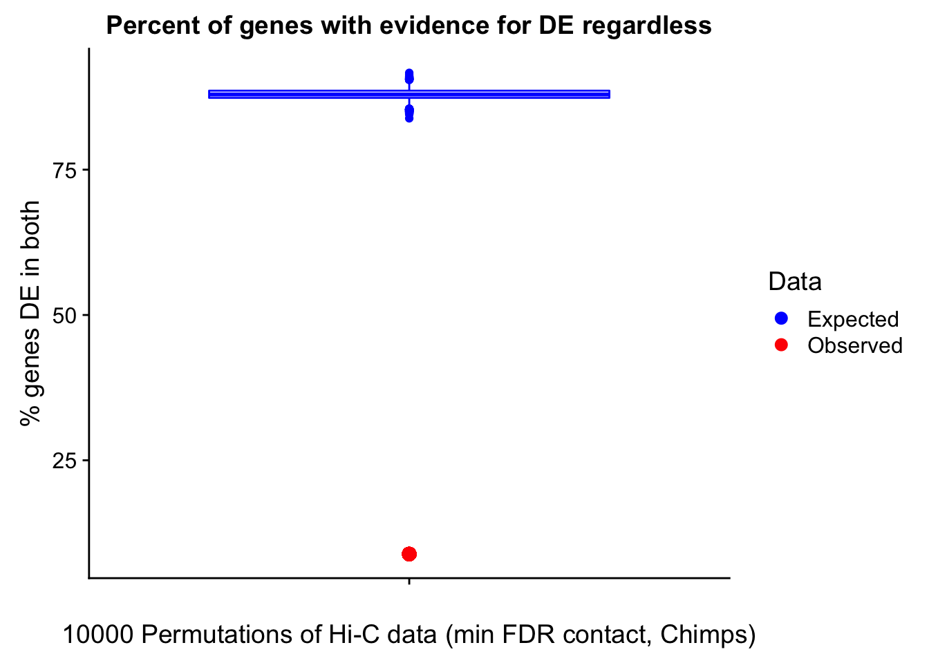
perm.vis("permout_c_maxB_DE", cmaxBDE, meta.data, "(max beta contact, Chimps)", DE=TRUE)
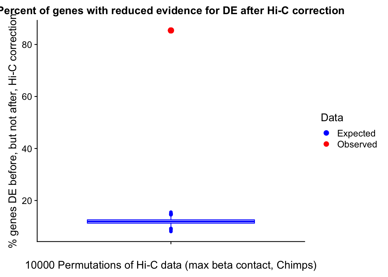
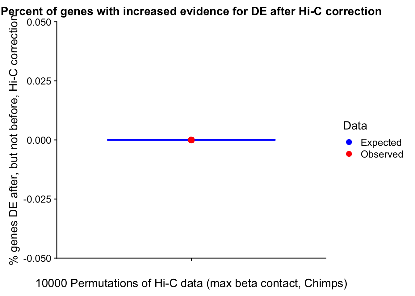

perm.vis("permout_c_US_DE", cUSDE, meta.data, "(upstream contact, Chimps)", DE=TRUE)

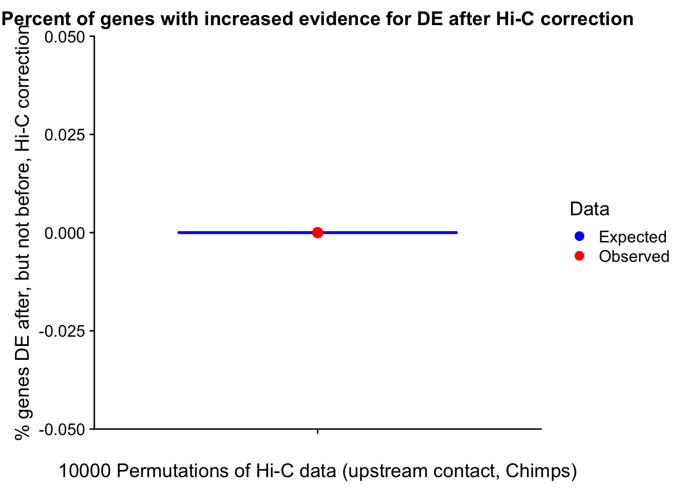
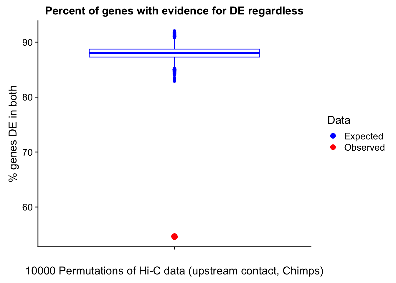 The permutations reveal that the observed data does appear pretty significant: it falls well outside the range of the distributions in each of the categories. The most important is showing that many more genes lose their DE status after regressing out Hi-C data in the observed case as compared to the permutations.
Exploration of higher-order structure in relation to gene expression. A/B Compartment Analysis
Here, I look at A/B compartment calls from HOMER and see if DE and/or DC genes are more likely to be in different compartments between species.
###Start with A/B compartments; much simpler. Read them in!
A_AB <- fread("~/Desktop/Hi-C/AB_compartments/50kb/A-21792.PC1.txt", header = TRUE, data.table=FALSE)
B_AB <- fread("~/Desktop/Hi-C/AB_compartments/50kb/B-28126.PC1.txt", header = TRUE, data.table=FALSE)
E_AB <- fread("~/Desktop/Hi-C/AB_compartments/50kb/E-28815.PC1.txt", header = TRUE, data.table=FALSE)
F_AB <- fread("~/Desktop/Hi-C/AB_compartments/50kb/F-28834.PC1.txt", header = TRUE, data.table=FALSE)
C_AB <- fread("~/Desktop/Hi-C/AB_compartments/50kb/C-3649.PC1.txt", header = TRUE, data.table=FALSE)
D_AB <- fread("~/Desktop/Hi-C/AB_compartments/50kb/D-40300.PC1.txt", header = TRUE, data.table=FALSE)
G_AB <- fread("~/Desktop/Hi-C/AB_compartments/50kb/G-3624.PC1.txt", header = TRUE, data.table=FALSE)
H_AB <- fread("~/Desktop/Hi-C/AB_compartments/50kb/H-3651.PC1.txt", header = TRUE, data.table=FALSE)

colnames(A_AB) <- colnames(B_AB) <- colnames(C_AB) <- colnames(D_AB) <- colnames(E_AB) <- colnames(F_AB) <- colnames(G_AB) <- colnames(H_AB) <- c("peakID", "chr", "start", "end", "strand", "PC1")

#Interestingly, within a species they're not all the same length (which doesn't make much sense as I thought these were identical genomes). A and F are females, B and E are males, so that's why B and E are larger--just remove chrY data to deal with that. But why aren't B and E identical, or A and F identical? Perhaps this is because not every individual gets enough reads at each of the regions to call compartments? Not really clear to me...for now, use ALL regions I can by combining these DFs, taking the mean PC1 value across individuals for those hits which ARE repeated (should be the vast majority).
humans.AB <- rbind(A_AB, B_AB, E_AB, F_AB)
humans.AB <- group_by(humans.AB, peakID) %>% summarise(chr=unique(chr), start=unique(start), end=unique(end), strand=unique(strand), PC1=mean(PC1))

chimps.AB <- rbind(C_AB, D_AB, G_AB, H_AB)
chimps.AB <- group_by(chimps.AB, peakID) %>% summarise(chr=unique(chr), start=unique(start), end=unique(end), strand=unique(strand), PC1=mean(PC1))

#Now, I want to assign a compartment (A or B) to each of these loci, so that they can then be examined WRT the Hi-C bins that might overlap them.
humans.AB$compartment <- ifelse(humans.AB$PC1>0, "A", "B")
chimps.AB$compartment <- ifelse(chimps.AB$PC1>0, "A", "B")

#Really, only want to look at genes we can actually call DE on based on expression levels, so only care about those genes in detable object. Can extract their exact positions from hgene.hic and cgene.hic and create peakIDs for them that match the AB compartment peak names. Basically, I just want to call which of the AB compartment peak bins they'll fall into. Note that those compartments were made 50kb at a time, so I need to round to lower 50k (or higher, depending on strand and proximity to boundary!) to figure out which compartment a gene belongs to.
colnames(hgene.hic) <- c("Hchr", "Hstart", "Hend", "genes", "Hplace", "Hstrand", "binchr", "binstart", "binend", "bindist.TSS")
colnames(cgene.hic) <- c("Cchr", "Cstart", "Cend", "genes", "Cplace", "Cstrand", "binchr", "binstart", "binend", "bindist.TSS")

#Add in lengths for appropriate PCA bin assignment in next part.
colnames(human_lengths) <- colnames(chimp_lengths) <- c("genes", "length")
hgene.PCA <- left_join(hgene.hic, human_lengths, by="genes")
cgene.PCA <- left_join(cgene.hic, chimp_lengths, by="genes")

#Assign genes to A/B compartment bins based on their position along the 50kb interval and their gene length, as well as strand orientation (trying to get the gene body in the actual 50kb interval).
hgene.PCA$HID <- paste(hgene.PCA$Hchr, ifelse(hgene.PCA$Hstrand=="+", ifelse(hgene.PCA$Hstart%%50000>=(50000-hgene.PCA$length), as.integer(50000*ceiling(hgene.PCA$Hstart/50000)), as.integer(50000*floor(hgene.PCA$Hstart/50000))), ifelse(hgene.PCA$Hstart%%50000<=hgene.PCA$length, as.integer((50000*floor(hgene.PCA$Hstart/50000)-50000)), as.integer(50000*floor(hgene.PCA$Hstart/50000)))), sep="-")
cgene.PCA$CID <- paste(cgene.PCA$Cchr, ifelse(cgene.PCA$Cstrand=="+", ifelse(cgene.PCA$Cstart%%50000>=(50000-cgene.PCA$length), as.integer(50000*ceiling(cgene.PCA$Cstart/50000)), as.integer(50000*floor(cgene.PCA$Cstart/50000))), ifelse(cgene.PCA$Cstart%%50000<=cgene.PCA$length, as.integer((50000*floor(cgene.PCA$Cstart/50000)-50000)), as.integer(50000*floor(cgene.PCA$Cstart/50000)))), sep="-")
#hgene.hic$HID <- ifelse(hgene.hic$Hstrand=="+", paste(hgene.hic$Hchr, as.integer(50000*floor(hgene.hic$Hstart/50000)), sep="-"))
#cgene.hic$CID <- paste(cgene.hic$Cchr, as.integer(50000*floor(cgene.hic$Cstart/50000)), sep="-")
hgenes.compartments <- select(hgene.PCA, Hchr, Hstart, genes, Hstrand, HID)
cgenes.compartments <- select(cgene.PCA, Cchr, Cstart, genes, Cstrand, CID)
compartment.genes <- left_join(detable, hgenes.compartments, by="genes") %>% left_join(., cgenes.compartments, by="genes")

#See how many genes fall within 5 kb of one of the boundaries here (at every 50kb interval): Though this was only considering the lower end, not if they fall on the other edge of the boundary (45k modulo remainder is equivalent and comparable #s!). REALLY what I should care about are positive strand genes falling at the upper edge of a boundary (implying their gene body may lie in the next compartment) and negative strand genes falling at the lower edge of a boundary (implying their gene body may lie in the previous compartment). If I have positive strand genes near the beginning or negative strand genes near the end that's not really an issue as their gene bodies should lie entirely within the compartment. It's really just those two specific cases.
sum((compartment.genes$Hstart%%50000)<=5000, na.rm=TRUE)
[1] 1065sum((compartment.genes$Cstart%%50000)<=5000, na.rm=TRUE)[1] 1094#In both species, roughly 1k of the genes we can consider at all fall near (w/in 5kb) one of the A/B boundaries we've established here. Could there be issues with pos/neg strand and how close they are to the boundary? I can check on this...or can also assume it's balanced across both issues. If the results from a naive analysis don't look good I can go back and fix this part of that.
#Now, merge compartment.genes and the humans.AB and chimps.AB compartment assignment DFs!
HAB <- select(humans.AB, peakID, compartment, PC1)
CAB <- select(chimps.AB, peakID, compartment, PC1)
colnames(HAB) <- c("HID", "compartment.H", "PC.H")
colnames(CAB) <- c("CID", "compartment.C", "PC.C")
final.AB <- left_join(compartment.genes, HAB, by="HID") %>% left_join(., CAB, by="CID")
final.AB$comp.diff <- ifelse(final.AB$compartment.H==final.AB$compartment.C, "no", "yes") #Note that 311 of these rows have missing data from at least one species so this determination can't be made? Often b/c of being on a scaffold in chimps.
final.AB$PC.diff <- abs(final.AB$PC.H-final.AB$PC.C)
final.AB <- final.AB[order(final.AB$adj.P.Val),]
final.AB$DE <- ifelse(final.AB$adj.P.Val<=0.05, "yes", "no")
table(final.AB$DE, final.AB$comp.diff, dnn=c("DE?", "Different Compartment b/t Species?")) Different Compartment b/t Species?
DE? no yes
no 7861 699
yes 2026 175chisq.test(table(final.AB$DE, final.AB$comp.diff, dnn=c("DE?", "Same Compartment b/t Species?")))
    Pearson's Chi-squared test with Yates' continuity correction

data:  table(final.AB$DE, final.AB$comp.diff, dnn = c("DE?", "Same Compartment b/t Species?"))
X-squared = 0.081518, df = 1, p-value = 0.7753
#So roughly 7.9% of DE genes are in different compartments between species, whereas ~8.1% of non-DE genes are in different compartments between species...shitty! And not significant!
#Would be nice to know if the differential compartments between species are at least concentrated in those differential contacts b/t species?! Add a column of the DC status between species.
final.AB$DC <- ifelse(final.AB$genes %in% filter(gene.hic.filt, min_FDR.H<=0.05|min_FDR.C<=0.05)$genes, "yes", "no")
table(final.AB$DC, final.AB$comp.diff, dnn=c("DC?", "Different Compartment b/t Species?")) Different Compartment b/t Species?
DC? no yes
no 9267 831
yes 620 43chisq.test(table(final.AB$DC, final.AB$comp.diff, dnn=c("DC?", "Different Compartment b/t Species?")))
    Pearson's Chi-squared test with Yates' continuity correction

data:  table(final.AB$DC, final.AB$comp.diff, dnn = c("DC?", "Different Compartment b/t Species?"))
X-squared = 2.3066, df = 1, p-value = 0.1288
#Again, not significant...can see that the genes which are DC have ~6.5% of them in different compartments b/t species, while the non-DC ones have 8.2% of them in different compartments b/t species. Note that this is also the exact opposite result I was hoping for...
#So a simple classification system is not sufficient for A/B compartment changes between the species. What if I actually took the mean PC value and plotted the difference bewtween species vs decreasing significance? The final.AB df is already ordered by DE p-val, so can do this real quick simply:
ggplot(data=final.AB) + geom_line(aes(x=adj.P.Val, y=PC.diff)) + ggtitle("Absolute Difference of PC1 Ordered by DE Significance") + xlab("Decreasing DE Significance") + ylab("|PC1 Difference b/t Species|")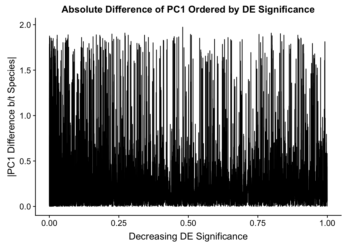
t.test(filter(final.AB, adj.P.Val<=0.05)$PC.diff, filter(final.AB, adj.P.Val>0.05)$PC.diff)
    Welch Two Sample t-test

data:  filter(final.AB, adj.P.Val <= 0.05)$PC.diff and filter(final.AB, adj.P.Val > 0.05)$PC.diff
t = -0.41452, df = 3592.6, p-value = 0.6785
alternative hypothesis: true difference in means is not equal to 0
95 percent confidence interval:
 -0.01694799  0.01103238
sample estimates:
mean of x mean of y
0.2271048 0.2300626
ggplot(data=final.AB) + geom_violin(aes(group=DE, x=DE, y=PC.diff), draw_quantiles = c(0.25, 0.5, 0.75)) + ggtitle("Absolute Difference of PC1 | DE") + xlab("DE Status") + ylab("|PC1 Difference b/t Species|")Warning: Removed 313 rows containing non-finite values (stat_ydensity).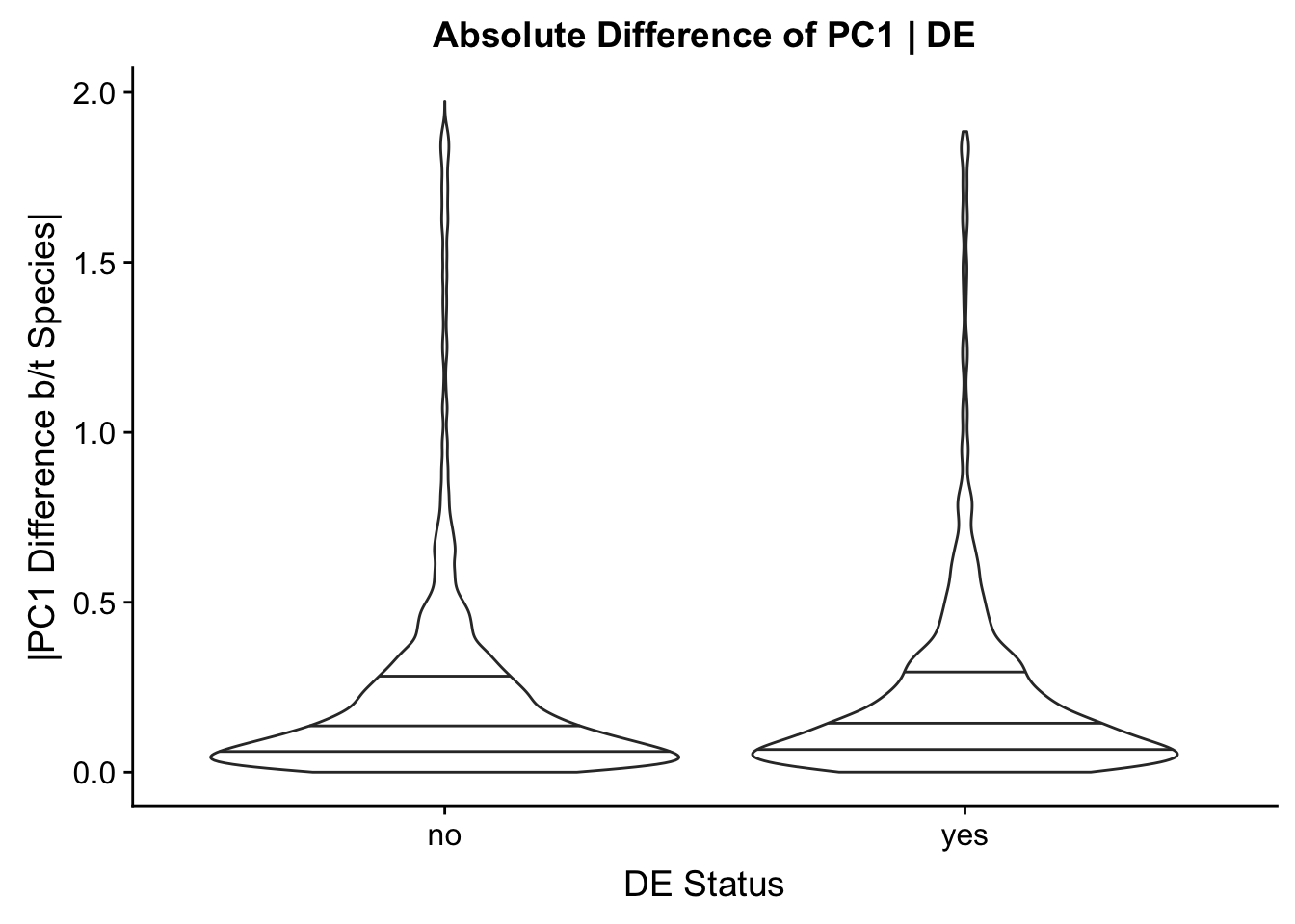
#None of this is particularly encouraging...but what if I did it on DC status? Can just check on binary status here to see if it'll even be significant or not:
t.test(filter(final.AB, DC=="yes")$PC.diff, filter(final.AB, DC=="no")$PC.diff)
    Welch Two Sample t-test

data:  filter(final.AB, DC == "yes")$PC.diff and filter(final.AB, DC == "no")$PC.diff
t = 1.1368, df = 750.12, p-value = 0.256
alternative hypothesis: true difference in means is not equal to 0
95 percent confidence interval:
 -0.01033890  0.03878608
sample estimates:
mean of x mean of y
0.2428049 0.2285813
#Aaaaand it's not. My inclination is to not spend any more time on the PCA element of this since the results don't seem to be good at all...
#Just a quick check to see if not using absolute difference would be better?
final.AB$PC.hdiff <- final.AB$PC.C-final.AB$PC.H
ggplot(data=final.AB) + geom_line(aes(x=adj.P.Val, y=PC.hdiff)) + ggtitle("Difference of PC1 Ordered by DE Significance") + xlab("Decreasing DE Significance") + ylab("PC1 Difference b/t Species (H-C)")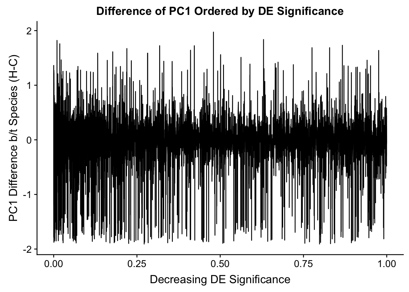
t.test(filter(final.AB, adj.P.Val<=0.05)$PC.hdiff, filter(final.AB, adj.P.Val>0.05)$PC.hdiff)
    Welch Two Sample t-test

data:  filter(final.AB, adj.P.Val <= 0.05)$PC.hdiff and filter(final.AB, adj.P.Val > 0.05)$PC.hdiff
t = -0.77796, df = 3544.3, p-value = 0.4366
alternative hypothesis: true difference in means is not equal to 0
95 percent confidence interval:
 -0.02450552  0.01058275
sample estimates:
  mean of x   mean of y
-0.03009098 -0.02312960
ggplot(data=final.AB) + geom_violin(aes(group=DE, x=DE, y=PC.hdiff), draw_quantiles = c(0.25, 0.5, 0.75)) + ggtitle("Difference of PC1 | DE") + xlab("DE Status") + ylab("PC1 Difference b/t Species (H-C)")Warning: Removed 313 rows containing non-finite values (stat_ydensity).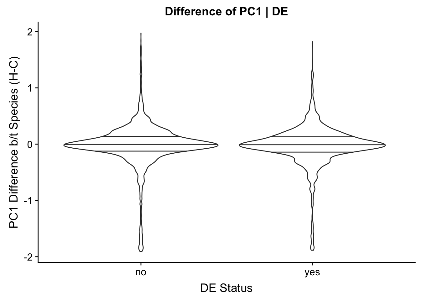
#None of this is particularly encouraging...but what if I did it on DC status? Can just check on binary status here to see if it'll even be significant or not:
t.test(filter(final.AB, DC=="yes")$PC.hdiff, filter(final.AB, DC=="no")$PC.hdiff) #Interestingly, if starting with humans as baseline here, this p-val is ALMOST significant!!!! Same if starting with chimps--just not using absolute value makes this almost significant...
    Welch Two Sample t-test

data:  filter(final.AB, DC == "yes")$PC.hdiff and filter(final.AB, DC == "no")$PC.hdiff
t = -1.9217, df = 747.95, p-value = 0.05503
alternative hypothesis: true difference in means is not equal to 0
95 percent confidence interval:
 -0.0609932583  0.0006511334
sample estimates:
  mean of x   mean of y
-0.05286562 -0.02269456
#Note that I also tried coloring the differences of PC1 plots by DC status and saw lines of both short and long variety, no clear trend of a bigger difference b/t species there, so no point in putting in the work to look at DC on x-axis.
#With the finished AB compartment DFs, should be as easy as just assigning Hi-C bins to A or B! Note that this current paradigm is limited to the genes that had direct overlap with a significant Hi-C bin; there's no reason for this! FIX! gene.hic.filt may not be the best data frame for this to work on then, since it doesn't include position information on all genes--get that!
# ABall <- select(gene.hic.filt, genes, logFC, AveExpr, adj.P.Val, B, HID, min_FDR_bin.H, CID, min_FDR_bin.C)
# hcomps <- select(humans.AB, peakID, compartment)
# ccomps <- select(chimps.AB, peakID, compartment)
# colnames(hcomps) <- c("HID", "compartment.H")
# colnames(ccomps) <- c("CID", "compartment.C")
# left_join(ABall, hcomps, by="HID") %>% left_join(., ccomps, by="CID") -> AB.all
#
# head(gene.hic.filt)
#Exploration of why they're not identically sized, not important. Also show some within-species exploration of the variance in these values; probably also not important. Collapsed.
# good.indices <- which(B_AB$`#peakID` %in% E_AB$`#peakID`)
# test <- B_AB[-good.indices,]
# good.indices <- which(E_AB$`#peakID` %in% B_AB$`#peakID`)
# test2 <- E_AB[-good.indices,]
#See how much within-species variance exists in these, after standardizing them to be identical across individuals from same species (remove X chromosome?). Or just do left joins on one and see what variance is like in that subset--most
# left_join(A_AB, B_AB, by="peakID") %>% left_join(., E_AB, by="peakID") %>% left_join(., F_AB, by="peakID") -> newtest
# newtest <- select(newtest, peakID, PC1.x, PC1.y, PC1.x.x, PC1.y.y)
# colnames(newtest) <- c("peakID", "A", "B", "E", "F")
# newtest$var <- apply(newtest[,-1], 1, var)
# ggplot(data=newtest) + geom_violin(aes(x="", y=var))
# sum(newtest$var>1, na.rm=TRUE) #Returns ~1000, so of about 54k rows there are 1000 with high variance between individuals. Leave it be for now, just something to think about in case this looks wonky later.
#Look at some candidates of the strongest compartment differences real quick to see if anything interesting here?
quantile(final.AB$PC.diff, probs=c(0.5, 0.6, 0.7, 0.8, 0.85, 0.9, 0.95, 0.99), na.rm = TRUE) 50% 60% 70% 80% 85% 90% 95%
0.1283966 0.1742264 0.2370739 0.3225847 0.3867206 0.4989470 0.7753319
99%
1.7327811 theonepercent <- which(final.AB$PC.diff>=1.7327811)
extremes <- final.AB[theonepercent,]
#I went back with some of this to look...nothing looks great TBH. For what it's worth, at least there are more instances in compartment differences where it's open in humans and closed in chimps than vice versa:
sum(final.AB$comp.diff=="yes"&final.AB$compartment.H=="A"&final.AB$compartment.C=="B", na.rm=TRUE) #Open in humans, closed in chimps[1] 513sum(final.AB$comp.diff=="yes"&final.AB$compartment.H=="B"&final.AB$compartment.C=="A", na.rm=TRUE) #Open in chimps, closed in humans[1] 361####25kb PCA A/B compartment analysis. Repeat this entire analysis utilizing 25kb as the window size for PCA calls.
###Start with A/B compartments; much simpler. Read them in!
A_AB <- fread("~/Desktop/Hi-C/AB_compartments/25kb/A-21792.PC1.txt", header = TRUE, data.table=FALSE)
B_AB <- fread("~/Desktop/Hi-C/AB_compartments/25kb/B-28126.PC1.txt", header = TRUE, data.table=FALSE)
E_AB <- fread("~/Desktop/Hi-C/AB_compartments/25kb/E-28815.PC1.txt", header = TRUE, data.table=FALSE)
F_AB <- fread("~/Desktop/Hi-C/AB_compartments/25kb/F-28834.PC1.txt", header = TRUE, data.table=FALSE)
C_AB <- fread("~/Desktop/Hi-C/AB_compartments/25kb/C-3649.PC1.txt", header = TRUE, data.table=FALSE)
D_AB <- fread("~/Desktop/Hi-C/AB_compartments/25kb/D-40300.PC1.txt", header = TRUE, data.table=FALSE)
G_AB <- fread("~/Desktop/Hi-C/AB_compartments/25kb/G-3624.PC1.txt", header = TRUE, data.table=FALSE)
H_AB <- fread("~/Desktop/Hi-C/AB_compartments/25kb/H-3651.PC1.txt", header = TRUE, data.table=FALSE)
colnames(A_AB) <- colnames(B_AB) <- colnames(C_AB) <- colnames(D_AB) <- colnames(E_AB) <- colnames(F_AB) <- colnames(G_AB) <- colnames(H_AB) <- c("peakID", "chr", "start", "end", "strand", "PC1")
#Interestingly, within a species they're not all the same length (which doesn't make much sense as I thought these were identical genomes). A and F are females, B and E are males, so that's why B and E are larger--just remove chrY data to deal with that. But why aren't B and E identical, or A and F identical? Perhaps this is because not every individual gets enough reads at each of the regions to call compartments? Not really clear to me...for now, use ALL regions I can by combining these DFs, taking the mean PC1 value across individuals for those hits which ARE repeated (should be the vast majority).
humans.AB <- rbind(A_AB, B_AB, E_AB, F_AB)
humans.AB <- group_by(humans.AB, peakID) %>% summarise(chr=unique(chr), start=unique(start), end=unique(end), strand=unique(strand), PC1=mean(PC1))
chimps.AB <- rbind(C_AB, D_AB, G_AB, H_AB)
chimps.AB <- group_by(chimps.AB, peakID) %>% summarise(chr=unique(chr), start=unique(start), end=unique(end), strand=unique(strand), PC1=mean(PC1))
#Now, I want to assign a compartment (A or B) to each of these loci, so that they can then be examined WRT the Hi-C bins that might overlap them.
humans.AB$compartment <- ifelse(humans.AB$PC1>0, "A", "B")
chimps.AB$compartment <- ifelse(chimps.AB$PC1>0, "A", "B")
#Really, only want to look at genes we can actually call DE on based on expression levels, so only care about those genes in detable object. Can extract their exact positions from hgene.hic and cgene.hic and create peakIDs for them that match the AB compartment peak names. Basically, I just want to call which of the AB compartment peak bins they'll fall into. Note that those compartments were made 50kb at a time, so I need to round to lower 50k (or higher, depending on strand and proximity to boundary!) to figure out which compartment a gene belongs to.
colnames(hgene.hic) <- c("Hchr", "Hstart", "Hend", "genes", "Hplace", "Hstrand", "binchr", "binstart", "binend", "bindist.TSS")
colnames(cgene.hic) <- c("Cchr", "Cstart", "Cend", "genes", "Cplace", "Cstrand", "binchr", "binstart", "binend", "bindist.TSS")
#Add in lengths for appropriate PCA bin assignment in next part.
colnames(human_lengths) <- colnames(chimp_lengths) <- c("genes", "length")
hgene.PCA <- left_join(hgene.hic, human_lengths, by="genes")
cgene.PCA <- left_join(cgene.hic, chimp_lengths, by="genes")
#Assign genes to A/B compartment bins based on their position along the 50kb interval and their gene length, as well as strand orientation (trying to get the gene body in the actual 50kb interval).
hgene.PCA$HID <- paste(hgene.PCA$Hchr, ifelse(hgene.PCA$Hstrand=="+", ifelse(hgene.PCA$Hstart%%25000>=(25000-hgene.PCA$length), as.integer(25000*ceiling(hgene.PCA$Hstart/25000)), as.integer(25000*floor(hgene.PCA$Hstart/25000))), ifelse(hgene.PCA$Hstart%%25000<=hgene.PCA$length, as.integer((25000*floor(hgene.PCA$Hstart/25000)-25000)), as.integer(25000*floor(hgene.PCA$Hstart/25000)))), sep="-")
cgene.PCA$CID <- paste(cgene.PCA$Cchr, ifelse(cgene.PCA$Cstrand=="+", ifelse(cgene.PCA$Cstart%%25000>=(25000-cgene.PCA$length), as.integer(25000*ceiling(cgene.PCA$Cstart/25000)), as.integer(25000*floor(cgene.PCA$Cstart/25000))), ifelse(cgene.PCA$Cstart%%25000<=cgene.PCA$length, as.integer((25000*floor(cgene.PCA$Cstart/25000)-25000)), as.integer(25000*floor(cgene.PCA$Cstart/25000)))), sep="-")
#hgene.hic$HID <- ifelse(hgene.hic$Hstrand=="+", paste(hgene.hic$Hchr, as.integer(25000*floor(hgene.hic$Hstart/25000)), sep="-"))
#cgene.hic$CID <- paste(cgene.hic$Cchr, as.integer(25000*floor(cgene.hic$Cstart/25000)), sep="-")
hgenes.compartments <- select(hgene.PCA, Hchr, Hstart, genes, Hstrand, HID)
cgenes.compartments <- select(cgene.PCA, Cchr, Cstart, genes, Cstrand, CID)
compartment.genes <- left_join(detable, hgenes.compartments, by="genes") %>% left_join(., cgenes.compartments, by="genes")
#See how many genes fall within 5 kb of one of the boundaries here (at every 50kb interval): Though this was only considering the lower end, not if they fall on the other edge of the boundary (45k modulo remainder is equivalent and comparable #s!). REALLY what I should care about are positive strand genes falling at the upper edge of a boundary (implying their gene body may lie in the next compartment) and negative strand genes falling at the lower edge of a boundary (implying their gene body may lie in the previous compartment). If I have positive strand genes near the beginning or negative strand genes near the end that's not really an issue as their gene bodies should lie entirely within the compartment. It's really just those two specific cases.
sum((compartment.genes$Hstart%%25000)<=5000, na.rm=TRUE)[1] 2167sum((compartment.genes$Cstart%%25000)<=5000, na.rm=TRUE)[1] 2182#In both species, roughly 1k of the genes we can consider at all fall near (w/in 5kb) one of the A/B boundaries we've established here. Could there be issues with pos/neg strand and how close they are to the boundary? I can check on this...or can also assume it's balanced across both issues. If the results from a naive analysis don't look good I can go back and fix this part of that.
#Now, merge compartment.genes and the humans.AB and chimps.AB compartment assignment DFs!
HAB <- select(humans.AB, peakID, compartment, PC1)
CAB <- select(chimps.AB, peakID, compartment, PC1)
colnames(HAB) <- c("HID", "compartment.H", "PC.H")
colnames(CAB) <- c("CID", "compartment.C", "PC.C")
final.AB <- left_join(compartment.genes, HAB, by="HID") %>% left_join(., CAB, by="CID")
final.AB$comp.diff <- ifelse(final.AB$compartment.H==final.AB$compartment.C, "no", "yes") #Note that 311 of these rows have missing data from at least one species so this determination can't be made? Often b/c of being on a scaffold in chimps.
final.AB$PC.diff <- abs(final.AB$PC.H-final.AB$PC.C)
final.AB <- final.AB[order(final.AB$adj.P.Val),]
final.AB$DE <- ifelse(final.AB$adj.P.Val<=0.05, "yes", "no")
table(final.AB$DE, final.AB$comp.diff, dnn=c("DE?", "Different Compartment b/t Species?")) Different Compartment b/t Species?
DE? no yes
no 7968 570
yes 2048 145chisq.test(table(final.AB$DE, final.AB$comp.diff, dnn=c("DE?", "Same Compartment b/t Species?")))
    Pearson's Chi-squared test with Yates' continuity correction

data:  table(final.AB$DE, final.AB$comp.diff, dnn = c("DE?", "Same Compartment b/t Species?"))
X-squared = 0.0035226, df = 1, p-value = 0.9527
#So roughly 6.61% of DE genes are in different compartments between species, whereas 6.68% of non-DE genes are in different compartments between species...shitty! And not significant!
#Would be nice to know if the differential compartments between species are at least concentrated in those differential contacts b/t species?! Add a column of the DC status between species.
final.AB$DC <- ifelse(final.AB$genes %in% filter(gene.hic.filt, min_FDR.H<=0.05|min_FDR.C<=0.05)$genes, "yes", "no")
table(final.AB$DC, final.AB$comp.diff, dnn=c("DC?", "Different Compartment b/t Species?")) Different Compartment b/t Species?
DC? no yes
no 9407 674
yes 609 41chisq.test(table(final.AB$DC, final.AB$comp.diff, dnn=c("DC?", "Different Compartment b/t Species?")))
    Pearson's Chi-squared test with Yates' continuity correction

data:  table(final.AB$DC, final.AB$comp.diff, dnn = c("DC?", "Different Compartment b/t Species?"))
X-squared = 0.086185, df = 1, p-value = 0.7691
#Again, not significant...can see that the genes which are DC have ~6.3% of them in different compartments b/t species, while the non-DC ones have 6.7% of them in different compartments b/t species. Note that this is also the exact opposite result I was hoping for...
#So a simple classification system is not sufficient for A/B compartment changes between the species. What if I actually took the mean PC value and plotted the difference bewtween species vs decreasing significance? The final.AB df is already ordered by DE p-val, so can do this real quick simply:
ggplot(data=final.AB) + geom_line(aes(x=adj.P.Val, y=PC.diff)) + ggtitle("Absolute Difference of PC1 Ordered by DE Significance") + xlab("Decreasing DE Significance") + ylab("|PC1 Difference b/t Species|")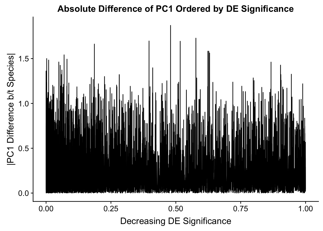
t.test(filter(final.AB, DE=="yes")$PC.diff, filter(final.AB, DE=="no")$PC.diff)
    Welch Two Sample t-test

data:  filter(final.AB, DE == "yes")$PC.diff and filter(final.AB, DE == "no")$PC.diff
t = 0.25904, df = 3489.3, p-value = 0.7956
alternative hypothesis: true difference in means is not equal to 0
95 percent confidence interval:
 -0.009105945  0.011878442
sample estimates:
mean of x mean of y
0.2175951 0.2162088
ggplot(data=final.AB) + geom_violin(aes(group=DE, x=DE, y=PC.diff), draw_quantiles = c(0.25, 0.5, 0.75)) + ggtitle("Absolute Difference of PC1 | DE") + xlab("DE Status") + ylab("|PC1 Difference b/t Species|")Warning: Removed 343 rows containing non-finite values (stat_ydensity).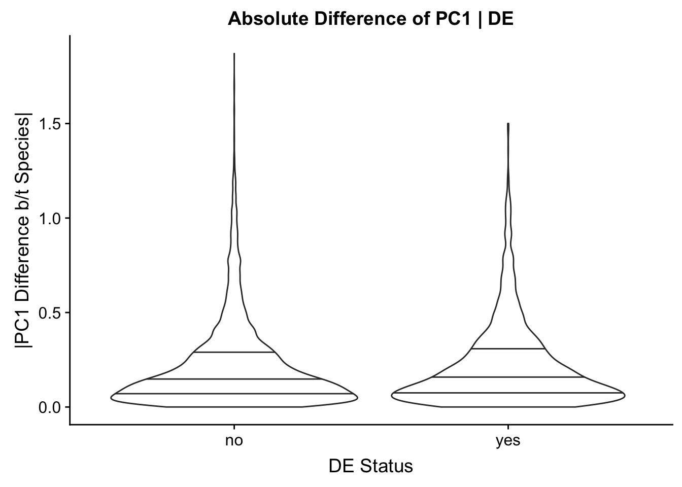
#None of this is particularly encouraging...but what if I did it on DC status? Can just check on binary status here to see if it'll even be significant or not:
t.test(filter(final.AB, DC=="yes")$PC.diff, filter(final.AB, DC=="no")$PC.diff)
    Welch Two Sample t-test

data:  filter(final.AB, DC == "yes")$PC.diff and filter(final.AB, DC == "no")$PC.diff
t = 2.6375, df = 726.52, p-value = 0.008531
alternative hypothesis: true difference in means is not equal to 0
95 percent confidence interval:
 0.006501246 0.044361584
sample estimates:
mean of x mean of y
0.2403831 0.2149517
#This time it is!...
ggplot(data=final.AB) + geom_violin(aes(group=DC, x=DC, y=PC.diff), draw_quantiles = c(0.25, 0.5, 0.75)) + ggtitle("Absolute Difference of PC1 | DC") + xlab("DC Status") + ylab("|PC1 Difference b/t Species|") + annotate("text", x=1.5, y=1, label="8.5 e - 3")Warning: Removed 343 rows containing non-finite values (stat_ydensity).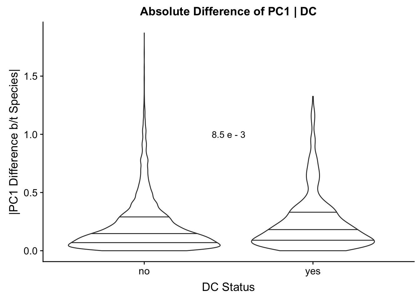
#table(final.AB$DC, final.AB$PC.diff, dnn=c("DC?", "Different Compartment b/t Species?")) Doesn't make sense here


#Just a quick check to see if not using absolute difference would be better?
final.AB$PC.hdiff <- final.AB$PC.C-final.AB$PC.H
ggplot(data=final.AB) + geom_line(aes(x=adj.P.Val, y=PC.hdiff)) + ggtitle("Difference of PC1 Ordered by DE Significance") + xlab("Decreasing DE Significance") + ylab("PC1 Difference b/t Species (H-C)")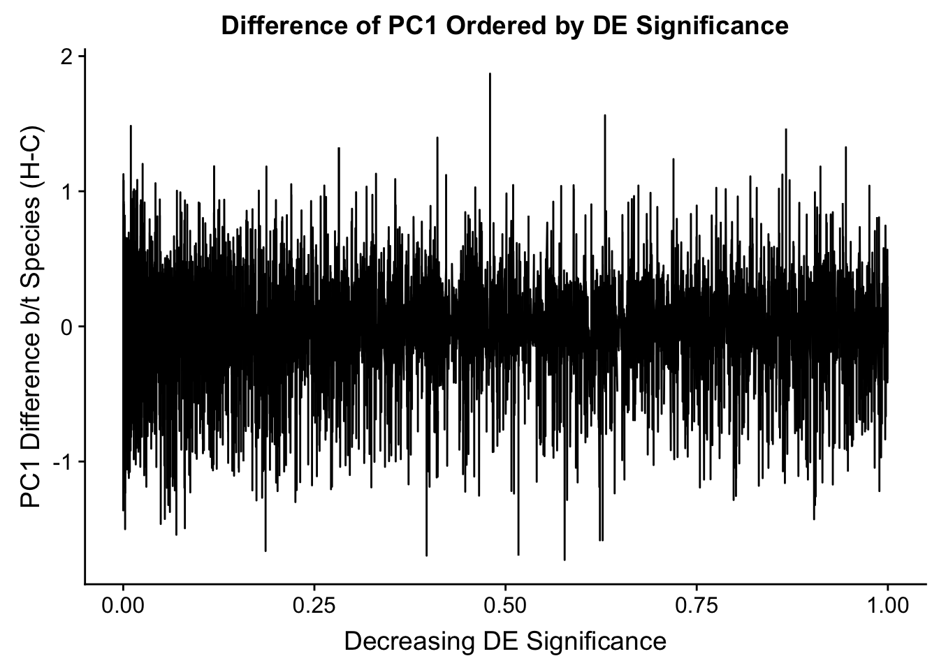
t.test(filter(final.AB, adj.P.Val<=0.05)$PC.hdiff, filter(final.AB, adj.P.Val>0.05)$PC.hdiff)
    Welch Two Sample t-test

data:  filter(final.AB, adj.P.Val <= 0.05)$PC.hdiff and filter(final.AB, adj.P.Val > 0.05)$PC.hdiff
t = -0.67607, df = 3442.5, p-value = 0.499
alternative hypothesis: true difference in means is not equal to 0
95 percent confidence interval:
 -0.019637088  0.009566943
sample estimates:
  mean of x   mean of y
-0.02171785 -0.01668278
ggplot(data=final.AB) + geom_violin(aes(group=DE, x=DE, y=PC.hdiff), draw_quantiles = c(0.25, 0.5, 0.75)) + ggtitle("Difference of PC1 | DE") + xlab("DE Status") + ylab("PC1 Difference b/t Species (H-C)")Warning: Removed 343 rows containing non-finite values (stat_ydensity).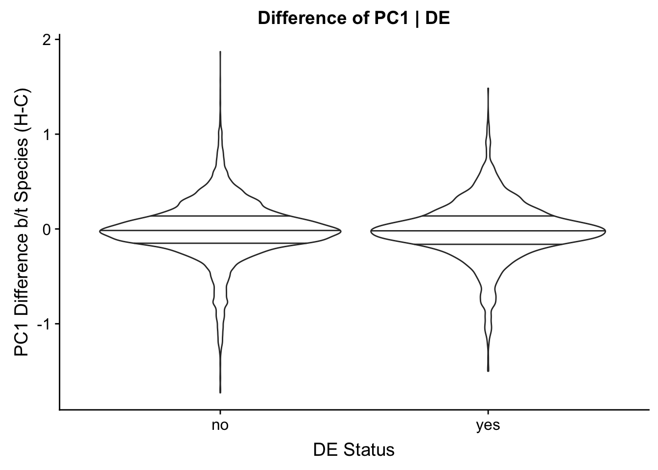
#None of this is particularly encouraging...but what if I did it on DC status? Can just check on binary status here to see if it'll even be significant or not:
t.test(filter(final.AB, DC=="yes")$PC.hdiff, filter(final.AB, DC=="no")$PC.hdiff)
    Welch Two Sample t-test

data:  filter(final.AB, DC == "yes")$PC.hdiff and filter(final.AB, DC == "no")$PC.hdiff
t = -3.2522, df = 724.08, p-value = 0.001198
alternative hypothesis: true difference in means is not equal to 0
95 percent confidence interval:
 -0.07021267 -0.01735265
sample estimates:
  mean of x   mean of y
-0.05884241 -0.01505974
#Overall, most of the A/B compartment calling results look rather atrocious...nothing much interesting to be gleaned here, unfortuantely.Differences in effect size/sign changes
This next section would be to look at differences in effect size and sign changes when doing the two separate lms (one before and one after regressing out Hi-C data from RPKM expression). Unfortunately the ash results I get have all their svalues as 1 so this is boring/not interesting right now. Hence it is not included. But let’s give it another go!
#######FRESH CODE 6-21-18#########
design <- model.matrix(~meta.data$SP)
exprs <- select(hmin, "A-21792", "B-28126", "C-3649", "D-40300", "E-28815", "F-28834", "G-3624", "H-3651", genes) #Should be done on just DE genes, filter with adj.P.Val<=0.05
hic <- select(hmin,"A_21792_HIC", "B_28126_HIC", "C_3649_HIC", "D_40300_HIC", "E_28815_HIC", "F_28834_HIC", "G_3624_HIC", "H_3651_HIC")
present <- sapply(1:nrow(hic), function(i) !any(is.na(hic[i,])))
genes <- exprs$genes
DEgenes <- filter(hmin, adj.P.Val<=0.05) %>% select(., genes)
myDEindices <- which(genes %in% DEgenes[,1])
exprs <- exprs[,-9]
exprs <- data.matrix(exprs[present,])
hic <- data.matrix(hic[present,])
designy <- as.factor(c("human", "human", "chimp", "chimp", "human", "human", "chimp", "chimp"))
colnames(hic) <- colnames(exprs)
hic <- as.data.table(hic)
exprs <- as.data.table(exprs)
test <- mediate.test.regressing(exprs, designy, hic)
Attaching package: 'assertthat'The following object is masked from 'package:tibble':
has_name#Shrink dat variance!
vshrDE <- vash(test$d_se[myDEindices], df=6)
vshrnonDE <- vash(test$d_se[-myDEindices], df=6)
vshrink <- vash(test$d_se, df=6)
#Separate out DE from non-DE genes:
DEtest <- test[myDEindices,]
nonDEtest <- test[-myDEindices,]
#Ash on DE genes
ash_reg <- ash(as.vector(DEtest$d), as.vector(vshrDE$sd.post), mixcompdist = "normal") #Now it works with this design coding. Use 6 df, as 2-group comparison and 8 individual samples (samples - 2)
summary(ash_reg$result$svalue<=0.05) #Incredible result, looks too good to be true. Mode FALSE TRUE
logical 1244 293 ind_sig <- (ash_reg$result$svalue < 0.05)
ind_sig[ind_sig == TRUE] <- "red"
ind_sig[ind_sig == FALSE] <- "black"
#FIG5A
plot(x=ash_reg$result$betahat, y=ash_reg$result$sebetahat, ylab="Standard error of the difference", xlab="Difference in Effect Size from 2 Linear Models", main="Difference of Effect Size in DE Genes", pch=16, cex=0.6, col=ind_sig, xlim=c(-4.5, 4.5), ylim=c(0, 3))
legend("topleft", legend=c("s < 0.05", "s >= 0.05"), col=c("red", "black"), pch=16:16, cex=0.8)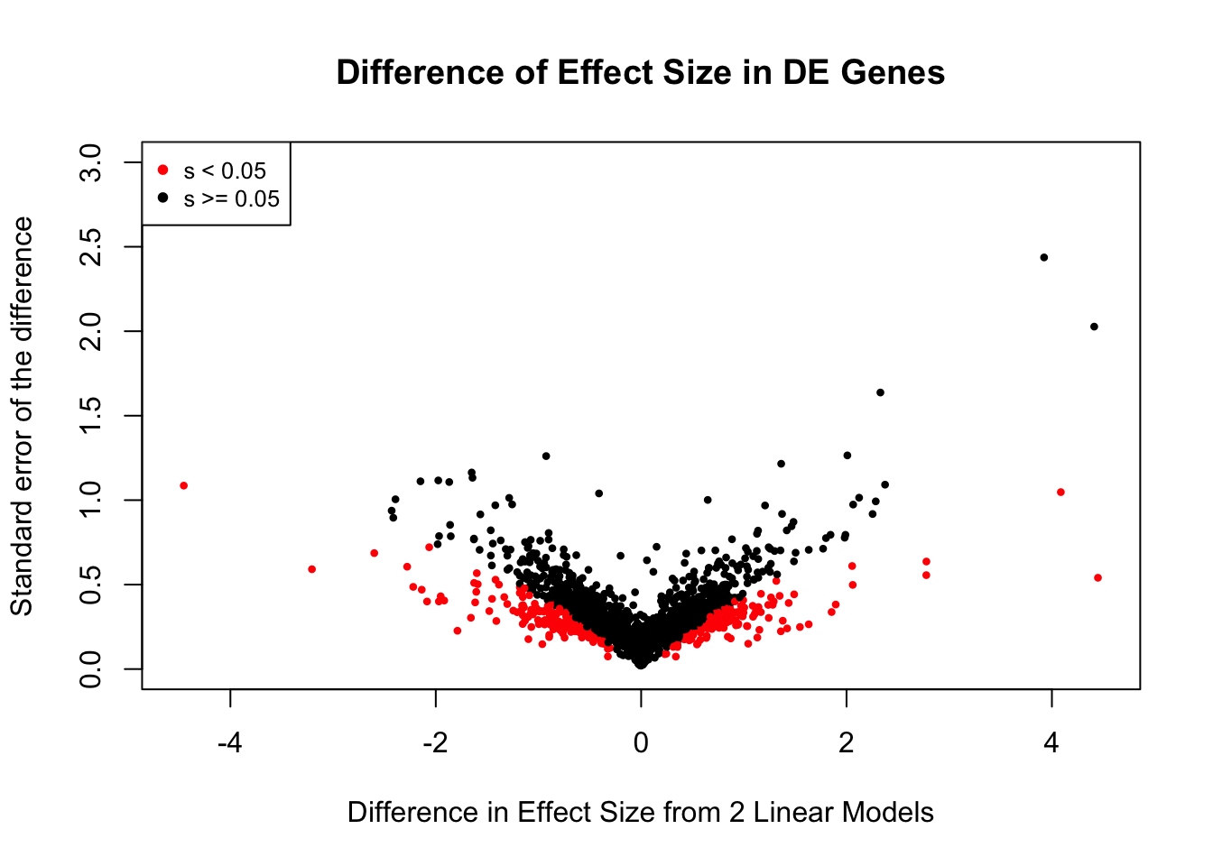
plot(ash_reg$result$betahat, -log10(ash_reg$result$svalue))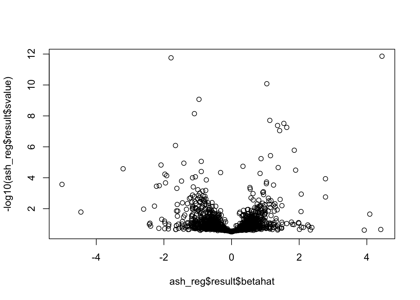
###### START EXAMPLE
#Figure out where some of these are to pull out good examples, try to find a dense region of them
myhits <- which(ash_reg$result$svalue<=0.05) #These SHOULD line up with DEtest indices...
realhits <- myDEindices[myhits] #Now go back to exprs original with these indices to get the gene names!
exprs <- select(hmin, "A-21792", "B-28126", "C-3649", "D-40300", "E-28815", "F-28834", "G-3624", "H-3651", genes) #Should be done on just DE genes, filter with adj.P.Val<=0.05
demgenes <- exprs[realhits,9]
testcases <- filter(gene.hic.filt, genes %in% demgenes)
table(testcases$genechr.H)
 chr1 chr10 chr11 chr12 chr13 chr14 chr15 chr16 chr17 chr18 chr19  chr2
   21    17    16    16     3     9    13    25    37     4    21     7
chr20 chr21 chr22  chr3  chr4  chr5  chr6  chr7  chr8  chr9  chrX
    9     3     7    17    12     8    18     7     7    12     4
testcases$sval <- ash_reg$result$svalue[myhits]
testcases <- testcases[order(testcases$sval),]
#Now, pull out expression values for those suckers:
options(scipen = 999)
mytest <- filter(humgenes, genes %in% testcases$genes)
mytest <- mytest[(mytest$genes %in% weighted.data$genes$genes),]
mean.species.expression <- as.data.frame(weighted.data$E) #Now, need to pull out the mean expression values for all those genes!
mean.species.expression$genes <- rownames(mean.species.expression)
mean.species.expression$Hmean <- rowMeans(mean.species.expression[,c(1:2,5:6)])
mean.species.expression$Cmean <- rowMeans(mean.species.expression[,c(3:4,7:8)])
mean.species.expression <- mean.species.expression[,(-1:-8)]
left_join(testcases, mean.species.expression, by="genes") -> filt.example
filter(filt.example, min_FDR.H<=0.05|min_FDR.C<=0.05) -> final.example
final.example$Hmean-final.example$Cmean [1] 4.5328579 1.2367448 1.4489860 2.4987542 -1.2978160 -1.4169804
[7] -3.1946646 -1.9931026 -1.9871103 1.1738427 -5.2288365 1.2336727
[13] -2.3053998 -1.0226005 0.9405034 -1.1595681 -0.8852151 -1.1076224
[19] 2.7855279 -1.4640895 -1.1098327 1.1607247 -1.0098363 -1.6114598
[25] -1.3898762 -0.8417933 1.8813176 -1.0449806 -1.1797100 1.3543069
[31] -1.5268885 -0.9104789 1.0591123 -3.0020201 -1.0473910 1.0138926
[37] -0.6466907 -4.7380406 -1.1886107 -0.6727022 4.2174090 0.8670641
[43] 0.8224821 -0.7521561 -0.6123475 0.6108439 -1.6004895 -0.4286268
[49] 1.0320064 0.7067310 0.7565189 -1.1045673 0.7209822 0.7714959
[55] 0.5101153 0.7215741 0.7052795 -0.8612434#gonna end up pulling 48th row example from final.example. Pull out its contact frequency vals for arc diagram creation:
final.example[48,] genes Length logFC AveExpr t P.Value
48 ENSG00000105486 6343 -0.4282247 6.929213 -3.293358 0.007383284
adj.P.Val B Hchr.H Hstart.H Hend.H Hstrand.H bin_pos.H
48 0.04020062 -3.034007 chr19 48110000 48120000 - 5444
genechr.H genepos.H HID min_FDR_bin.H min_FDR.H
48 chr19 48115444 chr19-48110000 chr19-47960000 0.0003698497
min_FDR_pval min_FDR_B.H median_FDR.H weighted_Z.ALLvar.H
48 0.000002316065 1.932498 0.2929028 0.09896256
weighted_Z.s2post.H fisher.H numcontacts.H max_B_bin.H max_B_FDR.H
48 0 69.32522 7 chr19-47960000 0.0003698497
max_B.H DS_bin.H DS_FDR.H DS_dist.H US_bin.H US_FDR.H
48 1.932498 chr19-48120000 0.1804779 10000 chr19-47970000 0.001113113
US_dist.H Hchr.C Hstart.C Hend.C Hstrand.C bin_pos.C genechr.C
48 140000 chr19 50210000 50220000 - 3062 chr19
genepos.C CID min_FDR_bin.C min_FDR.C min_FDR_B.C
48 50213062 chr19-50210000 chr19-50050000 0.0003698497 1.932498
median_FDR.C weighted_Z.ALLvar.C weighted_Z.s2post.C fisher.C
48 0.2929028 0.09896256 0 69.32522
numcontacts.C max_B_bin.C max_B_FDR.C max_B.C DS_bin.C
48 7 chr19-50050000 0.0003698497 1.932498 chr19-50220000
DS_FDR.C DS_dist.C US_bin.C US_FDR.C US_dist.C sval
48 0.1804779 10000 chr19-50060000 0.001113113 150000 0.03554588
Hmean Cmean
48 6.7149 7.143526which((data.filtered$H1=="chr17-64470000"|data.filtered$H2=="chr17-64470000")&(data.filtered$C1=="chr17-63970000"|data.filtered$C2=="chr17-63970000"))[1] 47406 49167 206246 207015 207030 251993 282314 283043which((data.filtered$H1=="chr17-64470000"&data.filtered$H2=="chr17-64430000")|(data.filtered$H2=="chr17-64470000"&data.filtered$H1=="chr17-64430000"))[1] 282314#Check on what other contacts might be significant in the region
QC <- filter(data.filtered, Hchr=="Chr. 17"&sp_BH_pval<=0.05)
QC$H1 <- gsub(".*-", "", QC$H1)
QC$H2 <- gsub(".*-", "", QC$H2)
which((QC$H1>=64400000&QC$H1<=64500000)&(QC$H2>=64400000&QC$H2<=64500000))[1] 218 323 397QC[c(218,323,397),] num-A H_chr1-A Hstart1-A Hend1-A Hstrand1-A H_chr2-A Hstart2-A Hend2-A
218 NA <NA> NA NA <NA> <NA> NA NA
323 NA <NA> NA NA <NA> <NA> NA NA
397 NA <NA> NA NA <NA> <NA> NA NA
Hstrand2-A C_chr1-A Cstart1-A Cend1-A Cstrand1-A C_chr2-A Cstart2-A
218 <NA> <NA> NA NA <NA> <NA> NA
323 <NA> <NA> NA NA <NA> <NA> NA
397 <NA> <NA> NA NA <NA> <NA> NA
Cend2-A Cstrand2-A InteractionID-A PeakID(1)-A chr(1)-A start(1)-A
218 NA <NA> <NA> <NA> <NA> NA
323 NA <NA> <NA> <NA> <NA> NA
397 NA <NA> <NA> <NA> <NA> NA
end(1)-A strand(1)-A Total_Reads(1)-A PeakID(2)-A chr(2)-A start(2)-A
218 NA <NA> NA <NA> <NA> NA
323 NA <NA> NA <NA> <NA> NA
397 NA <NA> NA <NA> <NA> NA
end(2)-A strand(2)-A Total_Reads(2)-A Distance-A Interaction_Reads-A
218 NA <NA> NA NA NA
323 NA <NA> NA NA NA
397 NA <NA> NA NA NA
Expected_Reads-A Z-score-A LogP-A FDR-A Circos_Thickness-A
218 NA NA NA NA NA
323 NA NA NA NA NA
397 NA NA NA NA NA
HCpair num-B
218 chr17-64430000_chr17-64470000/chr17-63920000_chr17-63970000 NA
323 chr17-64430000_chr17-64490000/chr17-63920000_chr17-63990000 NA
397 chr17-64420000_chr17-64500000/chr17-63910000_chr17-64000000 NA
H_chr1-B Hstart1-B Hend1-B Hstrand1-B H_chr2-B Hstart2-B Hend2-B
218 <NA> NA NA <NA> <NA> NA NA
323 <NA> NA NA <NA> <NA> NA NA
397 <NA> NA NA <NA> <NA> NA NA
Hstrand2-B C_chr1-B Cstart1-B Cend1-B Cstrand1-B C_chr2-B Cstart2-B
218 <NA> <NA> NA NA <NA> <NA> NA
323 <NA> <NA> NA NA <NA> <NA> NA
397 <NA> <NA> NA NA <NA> <NA> NA
Cend2-B Cstrand2-B InteractionID-B PeakID(1)-B chr(1)-B start(1)-B
218 NA <NA> <NA> <NA> <NA> NA
323 NA <NA> <NA> <NA> <NA> NA
397 NA <NA> <NA> <NA> <NA> NA
end(1)-B strand(1)-B Total_Reads(1)-B PeakID(2)-B chr(2)-B start(2)-B
218 NA <NA> NA <NA> <NA> NA
323 NA <NA> NA <NA> <NA> NA
397 NA <NA> NA <NA> <NA> NA
end(2)-B strand(2)-B Total_Reads(2)-B Distance-B Interaction_Reads-B
218 NA <NA> NA NA NA
323 NA <NA> NA NA NA
397 NA <NA> NA NA NA
Expected_Reads-B Z-score-B LogP-B FDR-B Circos_Thickness-B num-E
218 NA NA NA NA NA NA
323 NA NA NA NA NA NA
397 NA NA NA NA NA NA
H_chr1-E Hstart1-E Hend1-E Hstrand1-E H_chr2-E Hstart2-E Hend2-E
218 <NA> NA NA <NA> <NA> NA NA
323 <NA> NA NA <NA> <NA> NA NA
397 <NA> NA NA <NA> <NA> NA NA
Hstrand2-E C_chr1-E Cstart1-E Cend1-E Cstrand1-E C_chr2-E Cstart2-E
218 <NA> <NA> NA NA <NA> <NA> NA
323 <NA> <NA> NA NA <NA> <NA> NA
397 <NA> <NA> NA NA <NA> <NA> NA
Cend2-E Cstrand2-E InteractionID-E PeakID(1)-E chr(1)-E start(1)-E
218 NA <NA> <NA> <NA> <NA> NA
323 NA <NA> <NA> <NA> <NA> NA
397 NA <NA> <NA> <NA> <NA> NA
end(1)-E strand(1)-E Total_Reads(1)-E PeakID(2)-E chr(2)-E start(2)-E
218 NA <NA> NA <NA> <NA> NA
323 NA <NA> NA <NA> <NA> NA
397 NA <NA> NA <NA> <NA> NA
end(2)-E strand(2)-E Total_Reads(2)-E Distance-E Interaction_Reads-E
218 NA <NA> NA NA NA
323 NA <NA> NA NA NA
397 NA <NA> NA NA NA
Expected_Reads-E Z-score-E LogP-E FDR-E Circos_Thickness-E num-F
218 NA NA NA NA NA NA
323 NA NA NA NA NA NA
397 NA NA NA NA NA NA
H_chr1-F Hstart1-F Hend1-F Hstrand1-F H_chr2-F Hstart2-F Hend2-F
218 <NA> NA NA <NA> <NA> NA NA
323 <NA> NA NA <NA> <NA> NA NA
397 <NA> NA NA <NA> <NA> NA NA
Hstrand2-F C_chr1-F Cstart1-F Cend1-F Cstrand1-F C_chr2-F Cstart2-F
218 <NA> <NA> NA NA <NA> <NA> NA
323 <NA> <NA> NA NA <NA> <NA> NA
397 <NA> <NA> NA NA <NA> <NA> NA
Cend2-F Cstrand2-F InteractionID-F PeakID(1)-F chr(1)-F start(1)-F
218 NA <NA> <NA> <NA> <NA> NA
323 NA <NA> <NA> <NA> <NA> NA
397 NA <NA> <NA> <NA> <NA> NA
end(1)-F strand(1)-F Total_Reads(1)-F PeakID(2)-F chr(2)-F start(2)-F
218 NA <NA> NA <NA> <NA> NA
323 NA <NA> NA <NA> <NA> NA
397 NA <NA> NA <NA> <NA> NA
end(2)-F strand(2)-F Total_Reads(2)-F Distance-F Interaction_Reads-F
218 NA <NA> NA NA NA
323 NA <NA> NA NA NA
397 NA <NA> NA NA NA
Expected_Reads-F Z-score-F LogP-F FDR-F Circos_Thickness-F num-C
218 NA NA NA NA NA 236246
323 NA NA NA NA NA 238387
397 NA NA NA NA NA 241076
H_chr1-C Hstart1-C Hend1-C Hstrand1-C H_chr2-C Hstart2-C Hend2-C
218 chr17 64473558 64483581 + chr17 64425334 64435328
323 chr17 64493060 64502533 + chr17 64425334 64435328
397 chr17 64502533 64512511 + chr17 64415312 64425334
Hstrand2-C C_chr1-C Cstart1-C Cend1-C Cstrand1-C C_chr2-C Cstart2-C
218 + chr17 63970000 63980000 + chr17 63920000
323 + chr17 63990000 64000000 + chr17 63920000
397 + chr17 64000000 64010000 + chr17 63910000
Cend2-C Cstrand2-C InteractionID-C PeakID(1)-C chr(1)-C start(1)-C
218 63930000 + interaction1690 chr17-63970000 chr17 63970196
323 63930000 + interaction3831 chr17-63990000 chr17 63989573
397 63920000 + interaction6520 chr17-64000000 chr17 63998969
end(1)-C strand(1)-C Total_Reads(1)-C PeakID(2)-C chr(2)-C
218 63980196 + 4054 chr17-63920000 chr17
323 63999573 + 4108 chr17-63920000 chr17
397 64008969 + 4323 chr17-63910000 chr17
start(2)-C end(2)-C strand(2)-C Total_Reads(2)-C Distance-C
218 63920046 63930046 + 4096 50150
323 63919163 63929163 + 4096 70410
397 63910481 63920481 + 3824 88488
Interaction_Reads-C Expected_Reads-C Z-score-C LogP-C FDR-C
218 109 45.60180 3.071184 -34.82025 0.000000
323 83 36.13381 2.561925 -25.00079 0.000000
397 66 29.30642 2.237250 -19.51321 0.000018
Circos_Thickness-C num-D H_chr1-D Hstart1-D Hend1-D Hstrand1-D
218 10 276268 chr17 64473558 64483581 +
323 6 267998 chr17 64493060 64502533 +
397 4 272586 chr17 64502533 64512511 +
H_chr2-D Hstart2-D Hend2-D Hstrand2-D C_chr1-D Cstart1-D Cend1-D
218 chr17 64425334 64435328 + chr17 63970000 63980000
323 chr17 64425334 64435328 + chr17 63990000 64000000
397 chr17 64415312 64425334 + chr17 64000000 64010000
Cstrand1-D C_chr2-D Cstart2-D Cend2-D Cstrand2-D InteractionID-D
218 + chr17 63920000 63930000 + interaction10406
323 + chr17 63920000 63930000 + interaction2136
397 + chr17 63910000 63920000 + interaction6724
PeakID(1)-D chr(1)-D start(1)-D end(1)-D strand(1)-D
218 chr17-63970000 chr17 63970104 63980104 +
323 chr17-63990000 chr17 63989692 63999692 +
397 chr17-64000000 chr17 63998786 64008786 +
Total_Reads(1)-D PeakID(2)-D chr(2)-D start(2)-D end(2)-D
218 4438 chr17-63920000 chr17 63920229 63930229
323 4138 chr17-63920000 chr17 63919951 63929951
397 4609 chr17-63910000 chr17 63910226 63920226
strand(2)-D Total_Reads(2)-D Distance-D Interaction_Reads-D
218 + 4234 49875 74
323 + 4234 69741 76
397 + 4070 88560 59
Expected_Reads-D Z-score-D LogP-D FDR-D Circos_Thickness-D
218 39.91519 2.246405 -14.06295 0.002596 4
323 29.69296 2.986874 -27.98229 0.000000 8
397 26.54339 2.275882 -17.18421 0.000177 4
num-G H_chr1-G Hstart1-G Hend1-G Hstrand1-G H_chr2-G Hstart2-G
218 245433 chr17 64473558 64483581 + chr17 64425334
323 244589 chr17 64493060 64502533 + chr17 64425334
397 252103 chr17 64502533 64512511 + chr17 64415312
Hend2-G Hstrand2-G C_chr1-G Cstart1-G Cend1-G Cstrand1-G C_chr2-G
218 64435328 + chr17 63970000 63980000 + chr17
323 64435328 + chr17 63990000 64000000 + chr17
397 64425334 + chr17 64000000 64010000 + chr17
Cstart2-G Cend2-G Cstrand2-G InteractionID-G PeakID(1)-G chr(1)-G
218 63920000 63930000 + interaction2061 chr17-63970000 chr17
323 63920000 63930000 + interaction1217 chr17-63990000 chr17
397 63910000 63920000 + interaction8731 chr17-64000000 chr17
start(1)-G end(1)-G strand(1)-G Total_Reads(1)-G PeakID(2)-G
218 63970383 63980383 + 3709 chr17-63920000
323 63990457 64000457 + 4083 chr17-63920000
397 63998577 64008577 + 4402 chr17-63910000
chr(2)-G start(2)-G end(2)-G strand(2)-G Total_Reads(2)-G Distance-G
218 chr17 63919745 63929745 + 3841 50638
323 chr17 63919818 63929818 + 3841 70639
397 chr17 63911113 63921113 + 3362 87464
Interaction_Reads-G Expected_Reads-G Z-score-G LogP-G FDR-G
218 96 43.12241 2.837183 -26.95338 0.000000
323 93 37.05095 2.868164 -32.73931 0.000000
397 59 29.00601 1.984718 -14.34447 0.002335
Circos_Thickness-G num-H H_chr1-H Hstart1-H Hend1-H Hstrand1-H
218 8 237722 chr17 64473558 64483581 +
323 8 235932 chr17 64493060 64502533 +
397 4 236640 chr17 64502533 64512511 +
H_chr2-H Hstart2-H Hend2-H Hstrand2-H C_chr1-H Cstart1-H Cend1-H
218 chr17 64425334 64435328 + chr17 63970000 63980000
323 chr17 64425334 64435328 + chr17 63990000 64000000
397 chr17 64415312 64425334 + chr17 64000000 64010000
Cstrand1-H C_chr2-H Cstart2-H Cend2-H Cstrand2-H InteractionID-H
218 + chr17 63920000 63930000 + interaction2814
323 + chr17 63920000 63930000 + interaction1024
397 + chr17 63910000 63920000 + interaction1732
PeakID(1)-H chr(1)-H start(1)-H end(1)-H strand(1)-H
218 chr17-63970000 chr17 63970192 63980192 +
323 chr17-63990000 chr17 63990164 64000164 +
397 chr17-64000000 chr17 63998479 64008479 +
Total_Reads(1)-H PeakID(2)-H chr(2)-H start(2)-H end(2)-H
218 3929 chr17-63920000 chr17 63919979 63929979
323 4147 chr17-63920000 chr17 63919418 63929418
397 4593 chr17-63910000 chr17 63910629 63920629
strand(2)-H Total_Reads(2)-H Distance-H Interaction_Reads-H
218 + 3943 50213 92
323 + 3943 70746 94
397 + 3770 87850 80
Expected_Reads-H Z-score-H LogP-H FDR-H Circos_Thickness-H Hchr
218 42.68019 2.790360 -24.22792 0 6 Chr. 17
323 35.59823 3.097276 -36.03307 0 10 Chr. 17
397 31.38126 2.685398 -29.18700 0 8 Chr. 17
H1 H2 Cchr C1 C2 A-21792_norm
218 64430000 64470000 chr17 chr17-63920000 chr17-63970000 0.3205138
323 64430000 64490000 chr17 chr17-63920000 chr17-63990000 0.4236885
397 64420000 64500000 chr17 chr17-63910000 chr17-64000000 0.1031776
B-28126_norm C-3649_norm D-40300_norm E-28815_norm F-28834_norm
218 0.5313236 1.264110 0.8994624 0.6280133 0.4838557
323 0.3712357 1.204258 1.3677771 0.7631368 0.3003590
397 -0.1003274 1.181793 1.1611072 0.5462269 -0.2464347
G-3624_norm H-3651_norm Hmean Cmean ALLmean Hvar
218 1.148654 1.131268 0.49092659 1.110873 0.8009000 0.01650506
323 1.315510 1.429335 0.46460500 1.329220 0.8969125 0.04216332
397 1.017858 1.360370 0.07566058 1.180282 0.6279712 0.11896900
Cvar ALLvar found_in_H found_in_C disc_species tot_indiv_IDd
218 0.023339734 0.1268861 0 4 C 4
323 0.009104341 0.2355602 0 4 C 4
397 0.019727711 0.4080667 0 4 C 4
sp_beta sp_pval sp_BH_pval avg_IF t_statistic B_statistic
218 -0.6199468 0.001295658 0.03657103 0.8009000 -5.403267 -1.0625188
323 -0.8646150 0.000688142 0.02206974 0.8969125 -6.058465 -0.3645291
397 -1.1046213 0.001222219 0.03489531 0.6279712 -5.461487 -0.9981794
sx_pval btc_pval sx_beta btc_beta SE H1diff H2diff
218 0.1557771 0.4412829 0.18425022 0.09409531 0.1147355 23 6
323 0.8229855 0.4666735 0.03324526 0.11034517 0.1427119 527 6
397 0.7514995 0.6945329 0.06683261 0.08306741 0.2022565 22 22
C1diff C2diff Hdist Cdist dist_diff
218 NA NA 40000 50000 10000
323 NA NA 60000 70000 10000
397 NA NA 80000 90000 10000#filter(example, Hstart>=140500000&Hstart<=141500000) -> filt.example
hgenebed <- select(filt.example, genechr.H, genepos.H, Hmean)
cgenebed <- select(filt.example, genechr.C, genepos.C, Cmean)
hgenebed$end <- hgenebed$genepos.H+5000
cgenebed$end <- cgenebed$genepos.C+5000
hgenebed <- hgenebed[,c(1,2,4,3)]
cgenebed <- cgenebed[,c(1,2,4,3)]
cgenebed <- cgenebed[complete.cases(cgenebed),]
fwrite(hgenebed, "~/Desktop/Hi-C/pyGenomeTracks/filt.h.genes.bed", quote=FALSE, sep="\t", col.names =FALSE)
fwrite(cgenebed, "~/Desktop/Hi-C/pyGenomeTracks/filt.c.genes.bed", quote=FALSE, sep="\t", col.names =FALSE)
#Write out the appropriate columns from data.filtered to make an "arcs" file for visualization:
harcs <- filter(data.filtered, sp_beta>0, sp_BH_pval<=0.05) %>% select(., H1, H2, Hmean) #Note chr notation different due to other things changed; check on this later.
harcs$chr <- gsub("-.*", "", harcs$H1)
harcs$H1start <- as.numeric(gsub(".*-", "", harcs$H1))
harcs$H1end <- harcs$H1start+10000
harcs$H2start <- as.numeric(gsub(".*-", "", harcs$H2))
harcs$H2end <- harcs$H2start+10000
harcs <- harcs[,c(4:6, 4, 7:8, 3)]
harcs <- format(harcs, scientific=FALSE)
fwrite(harcs, "~/Desktop/Hi-C/pyGenomeTracks/RNAseq/humans.arcs", quote=FALSE, sep="\t", col.names=FALSE)
#Prep the same thing for chimpanzees:
carcs <- filter(data.filtered, sp_beta<0, sp_BH_pval<=0.05) %>% select(., C1, C2, Cmean) #Note chr notation different due to other things changed; check on this later.
carcs$chr <- gsub("-.*", "", carcs$C1)
carcs$C1start <- as.numeric(gsub(".*-", "", carcs$C1))
carcs$C1end <- carcs$C1start+10000
carcs$C2start <- as.numeric(gsub(".*-", "", carcs$C2))
carcs$C2end <- carcs$C2start+10000
carcs <- carcs[,c(4:6, 4, 7:8, 3)]
carcs <- format(carcs, scientific=FALSE)
fwrite(carcs, "~/Desktop/Hi-C/pyGenomeTracks/RNAseq/chimps.arcs", quote=FALSE, sep="\t", col.names=FALSE)
#Now add in an extra column placeholder so strand is in the right column for bedtools, and rearrange columns as well for bedtools' ease.
humgenes$placeholder <- "."
chimpgenes$placeholder <- "."
humgenes$Hend <- humgenes$Hstart+1
chimpgenes$Cend <- chimpgenes$Cstart+1
humgenes <- humgenes[,c(2:3, 6, 1, 5, 4)]
chimpgenes <- chimpgenes[,c(2:3, 6, 1, 5, 4)]
#Turn off scientific notation for writing the file out for bedtools to be able to use correctly.
options(scipen=999)
####### END EXAMPLE
#Now on non-DE genes
ash_reg_nonDE <- ash(as.vector(nonDEtest$d), as.vector(vshrnonDE$sd.post), mixcompdist = "normal") #Now it works with this design coding. Use 6 df, as 2-group comparison and 8 individual samples (samples - 2)Warning in estimate_mixprop(data, g, prior, optmethod = optmethod, control
= control, : Optimization failed to converge. Results may be unreliable.
Try increasing maxiter and rerunning.summary(ash_reg_nonDE$result$svalue<=0.05) #Incredible result, looks too good to be true. Mode FALSE
logical 6227 ind_sig <- (ash_reg_nonDE$result$svalue < 0.05)
ind_sig[ind_sig == TRUE] <- "red"
ind_sig[ind_sig == FALSE] <- "black"
#FIG5B
plot(x=ash_reg_nonDE$result$betahat, y=ash_reg_nonDE$result$sebetahat, ylab="Standard error of the difference", xlab="Difference in Effect Size from 2 Linear Models", main="Difference of Effect Size in non-DE Genes", pch=16, cex=0.6, col=ind_sig, xlim=c(-4.5, 4.5), ylim=c(0, 3))
legend("topleft", legend=c("s < 0.05", "s >= 0.05"), col=c("red", "black"), pch=16:16, cex=0.8)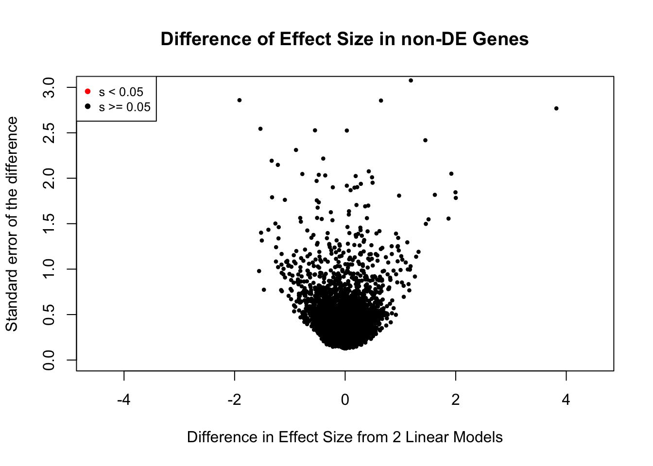
plot(ash_reg_nonDE$result$betahat, -log10(ash_reg_nonDE$result$svalue))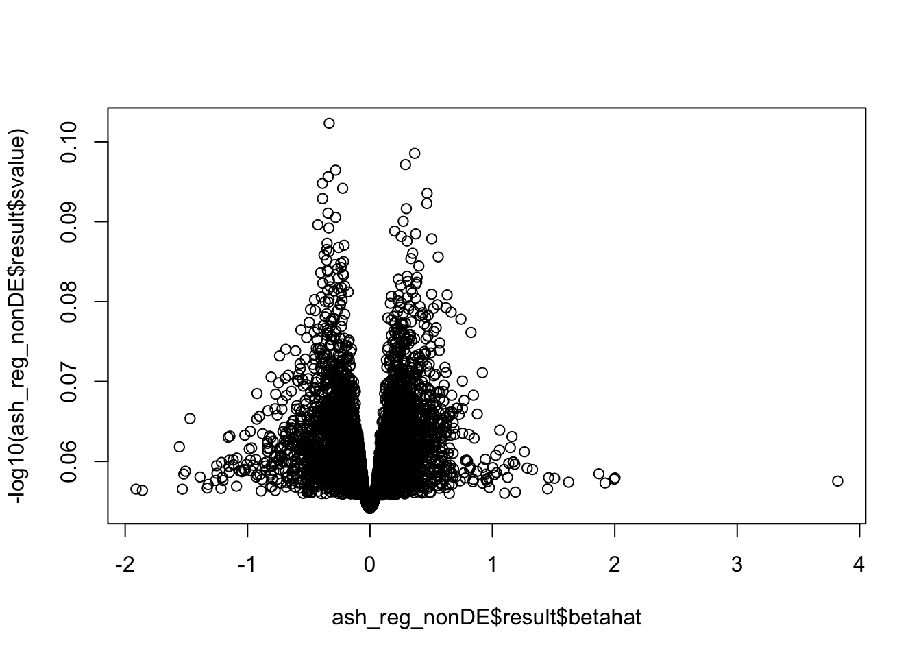
#Now on the full set, for comparison's sake.
ash_reg_full <- ash(as.vector(test$d), as.vector(vshrink$sd.post), mixcompdist = "normal") #Now it works with this design coding. Use 6 df, as 2-group comparison and 8 individual samples (samples - 2)
summary(ash_reg_full$result$svalue<=0.05) #Incredible result, looks too good to be true.
Mode FALSE TRUE
logical 7714 50 ind_sig <- (ash_reg_full$result$svalue < 0.05)
ind_sig[ind_sig == TRUE] <- "red"
ind_sig[ind_sig == FALSE] <- "black"
plot(x=ash_reg_full$result$betahat, y=ash_reg_full$result$sebetahat, ylab="Standard error of the difference", xlab="Difference in effect size from 2 lms", main="Difference of effect size (DE genes)", pch=16, cex=0.6, col=ind_sig)#, xlim=c(-2.5, 2.5), ylim=c(0, 1.3))
legend("topleft", legend=c("s < 0.05", "s >= 0.05"), col=c("red", "black"), pch=16:16, cex=0.8)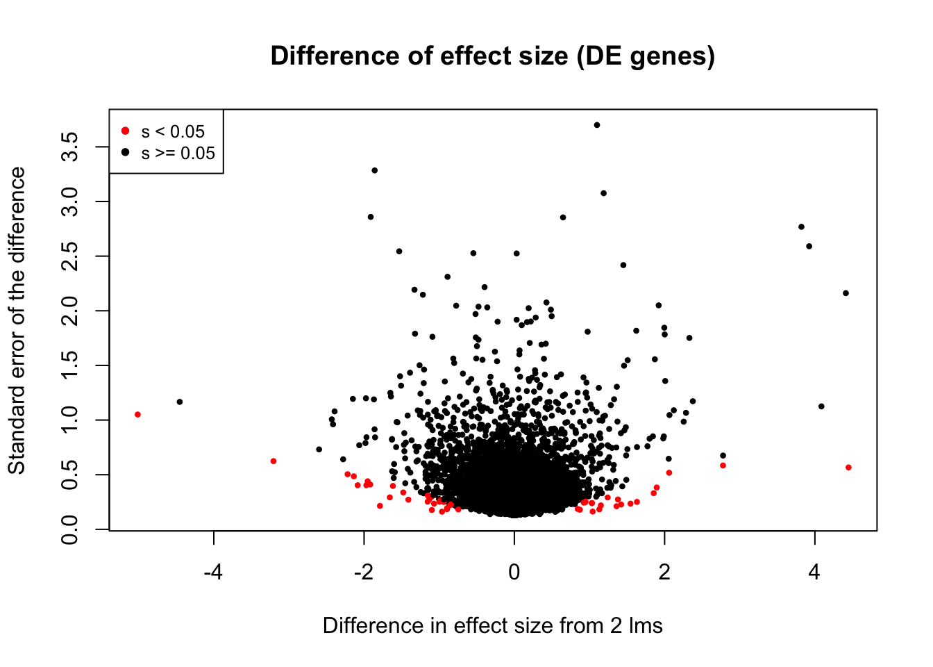
plot(ash_reg_full$result$betahat, -log10(ash_reg_full$result$svalue))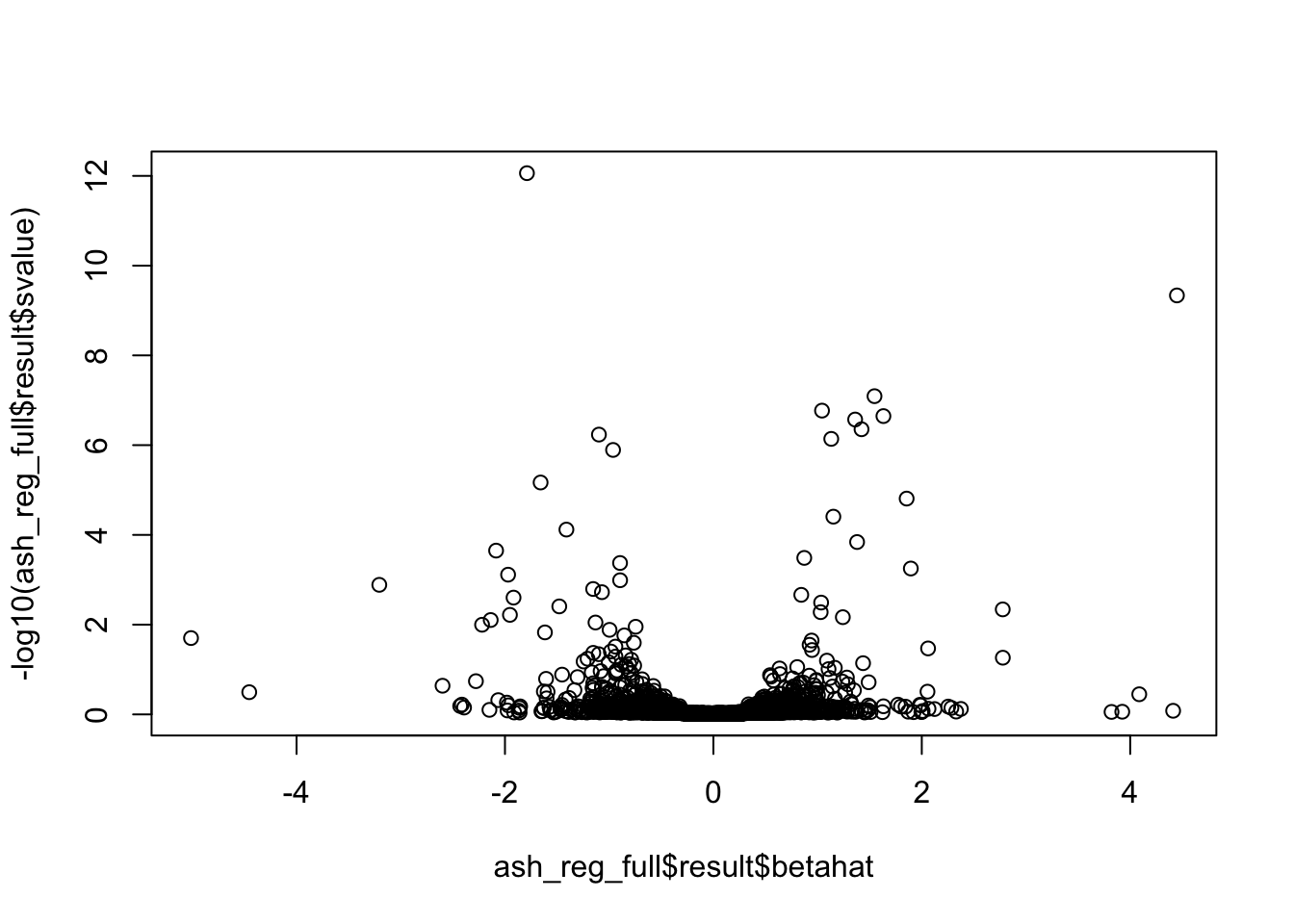
#Look at effect size shrinkage in full set ash vs. separated DE/nonDE ash:
plot(c(ash_reg$result$PosteriorMean, ash_reg_nonDE$result$PosteriorMean), ash_reg_full$result$PosteriorMean)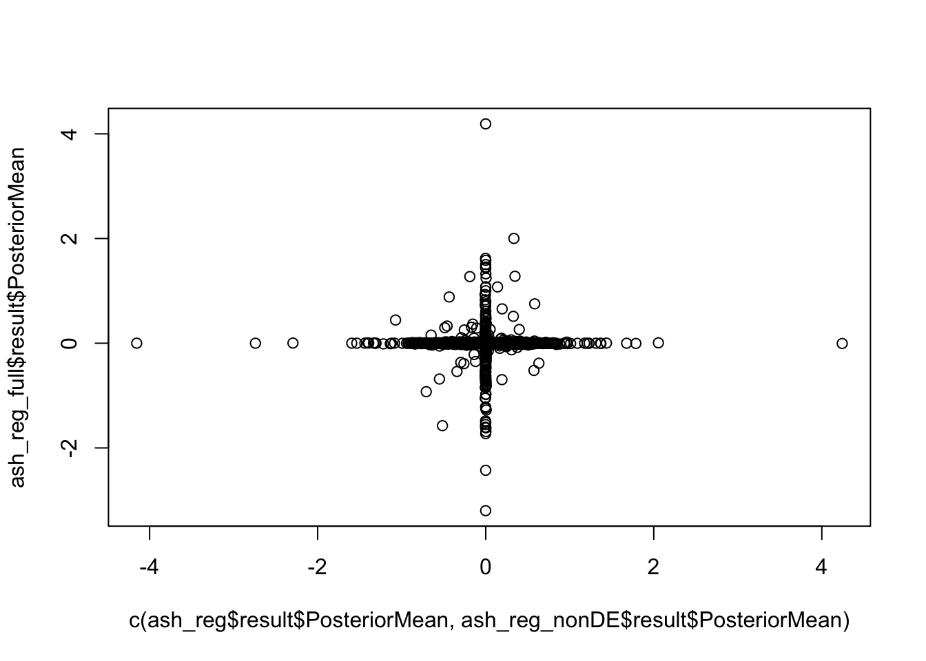
#Look at this just in DE:
plot(ash_reg$result$PosteriorMean, ash_reg_full$result$PosteriorMean[myDEindices])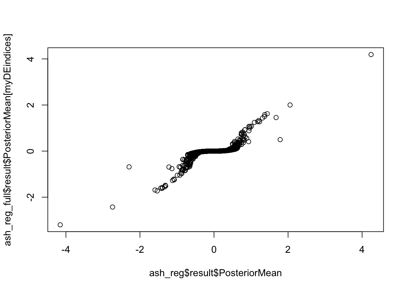
#Look at this just in non-DE:
plot(ash_reg_nonDE$result$PosteriorMean, ash_reg_full$result$PosteriorMean[-myDEindices])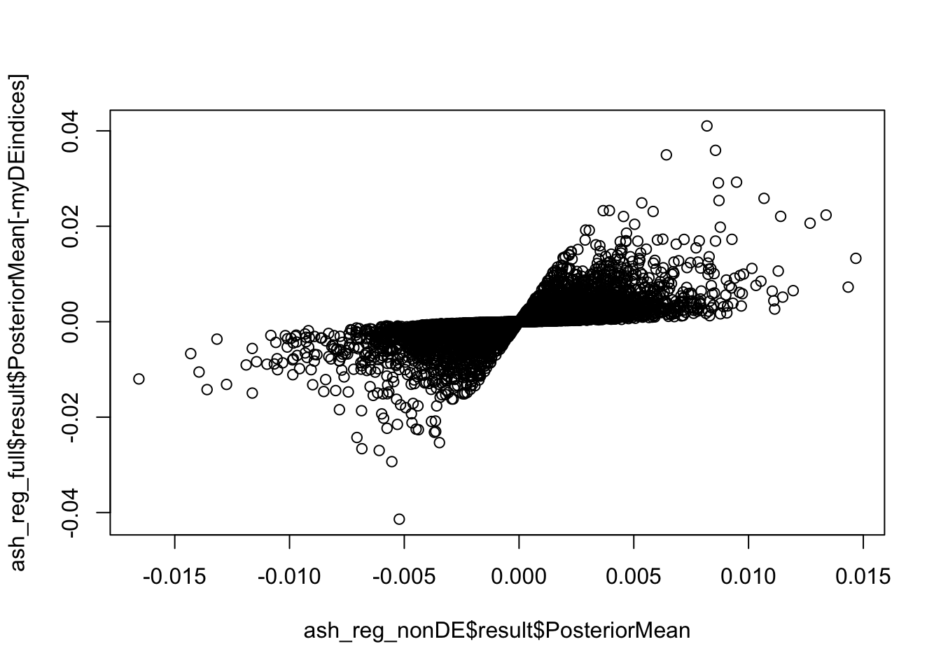
Mediation Review Questions
{r, include=FALSE, echo=FALSE} # #Simple plotting of logFC vs logFC. A positive logFC from the expression data indicates higher expression in humans. # #First, perform for entire set of genes, on non-DE and DE genes separately. # mydat <- select(gene.hic.filt, logFC, min_FDR_B.H, adj.P.Val, AveExpr) # ggplot(mydat) + geom_point(aes(x=logFC, y=min_FDR_B.H, color=adj.P.Val)) # ggplot(filter(mydat, adj.P.Val<=0.05)) + geom_point(aes(x=logFC, y=min_FDR_B.H)) + xlab("LogFC, Expression") + ylab("LogFC, Contact") + ggtitle("LogFC Expression vs. LogFC Contact for DE Genes") # ggplot(filter(mydat, adj.P.Val>0.05)) + geom_point(aes(x=logFC, y=min_FDR_B.H)) + xlab("LogFC, Expression") + ylab("LogFC, Contact") + ggtitle("LogFC Expression vs. LogFC Contact for non-DE Genes") # # #Now, take a look at what happens if I stratify things by which species it's more highly expressed in, and its DE status, and calculate R-squareds. Should do this with actual mean expression values per species # human.high.DE <- filter(mydat, logFC>0, adj.P.Val<=0.05) # human.high.nonDE <- filter(mydat, logFC>0, adj.P.Val>0.05) # chimp.high.DE <- filter(mydat, logFC<0, adj.P.Val<=0.05) # chimp.high.nonDE <- filter(mydat, logFC<0, adj.P.Val>0.05) # summary(lm(human.high.nonDE$logFC~human.high.nonDE$min_FDR_B.H))$adj.r.squared # summary(lm(human.high.DE$logFC~human.high.DE$min_FDR_B.H))$adj.r.squared # summary(lm(chimp.high.nonDE$logFC~chimp.high.nonDE$min_FDR_B.H))$adj.r.squared # summary(lm(chimp.high.DE$logFC~chimp.high.DE$min_FDR_B.H))$adj.r.squared # # # #Now, try out the suggested regression. # new.weighted.data <- weighted.data # new.weighted.data$E <- dge_final$lcpm_counts[,c(8, 6, 1, 4, 7, 5, 2, 3)] # # #Now, need to subset this down to the genes we have contact frequency for (from hmin table, created far below) # my.hmin <- select(hmin, genes, A_21792_HIC, B_28126_HIC, C_3649_HIC, D_40300_HIC, E_28815_HIC, F_28834_HIC, G_3624_HIC, H_3651_HIC) # deez.genes <- left_join(new.weighted.data$genes, my.hmin) # good.indices <- which(complete.cases(deez.genes)) # new.weighted.data <- new.weighted.data[good.indices,] # new.weighted.data$HiC <- deez.genes[good.indices, 3:10] # # meta.exp.data <- data.frame("SP"=c("C", "C", "C", "C", "H", "H", "H", "H"), "SX"=c("M","M" ,"F","F","F", "M","M","F")) # SP <- factor(meta.exp.data$SP,levels = c("H","C")) # # # for(row in 1:nrow(new.weighted.data$E)){ # lmFit() # } # exp.design <- model.matrix(~0+SP+new.weighted.data$HiC+SP:new.weighted.data$HiC)#(~1+meta.exp.data$SP+meta.exp.data$SX) But where does freq come from? # colnames(exp.design) <- c("Human", "Chimp") # weighted.data <- voom(new.weighted.data, exp.design, plot=TRUE, normalize.method = "cyclicloess") # # ##Obtain rest of LM results, with particular eye to DE table! # vfit <- lmFit(weighted.data, exp.design) # efit <- eBayes(vfit) # # mycon <- makeContrasts(HvC = Human-Chimp, levels = exp.design) # diff_species <- contrasts.fit(efit, mycon) # finalfit <- eBayes(diff_species) # detable <- topTable(finalfit, coef = 1, adjust.method = "BH", number = Inf, sort.by="none") #
sessionInfo()R version 3.4.0 (2017-04-21)
Platform: x86_64-apple-darwin15.6.0 (64-bit)
Running under: OS X El Capitan 10.11.6
Matrix products: default
BLAS: /Library/Frameworks/R.framework/Versions/3.4/Resources/lib/libRblas.0.dylib
LAPACK: /Library/Frameworks/R.framework/Versions/3.4/Resources/lib/libRlapack.dylib
locale:
[1] en_US.UTF-8/en_US.UTF-8/en_US.UTF-8/C/en_US.UTF-8/en_US.UTF-8
attached base packages:
[1] grid compiler stats graphics grDevices utils datasets
[8] methods base
other attached packages:
[1] assertthat_0.2.0 VennDiagram_1.6.20 futile.logger_1.4.3
[4] glmnet_2.0-16 foreach_1.4.4 Matrix_1.2-15
[7] medinome_0.0.1 vashr_0.99.1 qvalue_2.10.0
[10] SQUAREM_2017.10-1 ashr_2.2-32 forcats_0.4.0
[13] purrr_0.3.1 readr_1.3.1 tibble_2.0.1
[16] tidyverse_1.2.1 edgeR_3.20.9 RColorBrewer_1.1-2
[19] heatmaply_0.15.2 viridis_0.5.1 viridisLite_0.3.0
[22] stringr_1.4.0 gplots_3.0.1.1 Hmisc_4.2-0
[25] Formula_1.2-3 survival_2.43-3 lattice_0.20-38
[28] dplyr_0.8.0.1 plotly_4.8.0 cowplot_0.9.4
[31] ggplot2_3.1.0 reshape2_1.4.3 data.table_1.12.0
[34] tidyr_0.8.3 plyr_1.8.4 limma_3.34.9
loaded via a namespace (and not attached):
[1] colorspace_1.4-0 class_7.3-15 modeltools_0.2-22
[4] mclust_5.4.2 rprojroot_1.3-2 htmlTable_1.13.1
[7] base64enc_0.1-3 fs_1.2.6 rstudioapi_0.9.0
[10] flexmix_2.3-15 mvtnorm_1.0-8 lubridate_1.7.4
[13] xml2_1.2.0 codetools_0.2-16 splines_3.4.0
[16] pscl_1.5.2 doParallel_1.0.14 robustbase_0.92-8
[19] knitr_1.22 jsonlite_1.6 workflowr_1.2.0
[22] broom_0.5.1 cluster_2.0.7-1 kernlab_0.9-27
[25] httr_1.4.0 backports_1.1.3 lazyeval_0.2.1
[28] cli_1.0.1 formatR_1.6 acepack_1.4.1
[31] htmltools_0.3.6 tools_3.4.0 gtable_0.2.0
[34] glue_1.3.0 Rcpp_1.0.0 cellranger_1.1.0
[37] trimcluster_0.1-2.1 gdata_2.18.0 nlme_3.1-137
[40] iterators_1.0.10 fpc_2.1-11.1 xfun_0.5
[43] rvest_0.3.2 gtools_3.8.1 dendextend_1.9.0
[46] DEoptimR_1.0-8 MASS_7.3-51.1 scales_1.0.0
[49] TSP_1.1-6 hms_0.4.2 parallel_3.4.0
[52] lambda.r_1.2.3 yaml_2.2.0 gridExtra_2.3
[55] rpart_4.1-13 latticeExtra_0.6-28 stringi_1.3.1
[58] gclus_1.3.2 checkmate_1.9.1 seriation_1.2-3
[61] caTools_1.17.1.2 truncnorm_1.0-8 rlang_0.3.1
[64] pkgconfig_2.0.2 prabclus_2.2-7 bitops_1.0-6
[67] evaluate_0.13 labeling_0.3 htmlwidgets_1.3
[70] tidyselect_0.2.5 magrittr_1.5 R6_2.4.0
[73] generics_0.0.2 pillar_1.3.1 haven_2.1.0
[76] whisker_0.3-2 foreign_0.8-71 withr_2.1.2
[79] mixsqp_0.1-97 nnet_7.3-12 modelr_0.1.4
[82] crayon_1.3.4 futile.options_1.0.1 KernSmooth_2.23-15
[85] rmarkdown_1.11 locfit_1.5-9.1 readxl_1.3.0
[88] git2r_0.24.0 digest_0.6.18 diptest_0.75-7
[91] webshot_0.5.1 stats4_3.4.0 munsell_0.5.0
[94] registry_0.5-1