Biostatistical analysis part 2
AGC
2 2 2022
Last updated: 2022-02-21
Checks: 7 0
Knit directory: S:/KJP_Biolabor/Projects/scSeq_Hefendehl/
This reproducible R Markdown analysis was created with workflowr (version 1.7.0). The Checks tab describes the reproducibility checks that were applied when the results were created. The Past versions tab lists the development history.
Great! Since the R Markdown file has been committed to the Git repository, you know the exact version of the code that produced these results.
Great job! The global environment was empty. Objects defined in the global environment can affect the analysis in your R Markdown file in unknown ways. For reproduciblity it’s best to always run the code in an empty environment.
The command set.seed(20220131) was run prior to running the code in the R Markdown file. Setting a seed ensures that any results that rely on randomness, e.g. subsampling or permutations, are reproducible.
Great job! Recording the operating system, R version, and package versions is critical for reproducibility.
Nice! There were no cached chunks for this analysis, so you can be confident that you successfully produced the results during this run.
Great job! Using relative paths to the files within your workflowr project makes it easier to run your code on other machines.
Great! You are using Git for version control. Tracking code development and connecting the code version to the results is critical for reproducibility.
The results in this page were generated with repository version ef56d05. See the Past versions tab to see a history of the changes made to the R Markdown and HTML files.
Note that you need to be careful to ensure that all relevant files for the analysis have been committed to Git prior to generating the results (you can use wflow_publish or wflow_git_commit). workflowr only checks the R Markdown file, but you know if there are other scripts or data files that it depends on. Below is the status of the Git repository when the results were generated:
Ignored files:
    Ignored:    .Rproj.user/
    Ignored:    data/ReloadAllData_Hefendehl_Stroke_Dec'21.RData
    Ignored:    data/Sample_Tables/
    Ignored:    data/counts.csv
    Ignored:    data/genecounts.csv
    Ignored:    data/microglia_protein.rds
    Ignored:    data/samples.integrated.RData
    Ignored:    data/tx2genes.csv
    Ignored:    output/Descriptives.Rmd
    Ignored:    output/Descriptives.docx

Untracked files:
    Untracked:  app/
    Untracked:  geneviewer/
    Untracked:  genplotter/
    Untracked:  workflow_helper.R
Note that any generated files, e.g. HTML, png, CSS, etc., are not included in this status report because it is ok for generated content to have uncommitted changes.
There are no past versions. Publish this analysis with wflow_publish() to start tracking its development.
#get sample data
samples.integrated@meta.data %>% as.data.frame() -> samplemeta

# convert to correct data type

# define genotype as is
samplemeta$Genotype_corr = factor(samplemeta$Genotype=="wt", levels=c(F,T), labels = c("APPPS1+", "WT"))
samplemeta$Genotype_corr = relevel(samplemeta$Genotype_corr, ref="WT")

samplemeta$methoxy = factor(samplemeta$Genotype=="MX04+", levels=c(T,F), labels = c("MX04+", "MX04-"))

samplemeta$Treatment = as.factor(samplemeta$Treatment)
samplemeta$Treatment = relevel(samplemeta$Treatment, ref="Ctrl")
samplemeta$Mouse_ID = as.factor(samplemeta$Mouse_ID)
samplemeta$Sex = as.factor(samplemeta$Sex)
samplemeta$Brain_region = as.factor(samplemeta$Brain_region)
samplemeta$Celltype = as.factor(samplemeta$Celltype)

nCells=nrow(samplemeta)
nMice=nlevels(samplemeta$Mouse_ID)
nCelltypes=nlevels(samplemeta$Celltype)
Sample descriptive:
Data contains a total of 649 Cells from 9. Q: Original raw datset containing only frankfurt data included 1149 cells. What were the filter criteria in the primary cell type analysis
Cells per Mouse
Cells per Strain
table(Mouse_ID=samplemeta$Mouse_ID) %>% as.data.frame() %>% display_tab()| Mouse_ID | Freq |
|---|---|
| 23#15773 | 66 |
| 23#15774 | 49 |
| 23#15792 | 47 |
| 386 | 41 |
| 387 | 44 |
| 388 | 113 |
| 409 | 86 |
| 457 | 115 |
| 461 | 88 |
Cells per Genotype
table(Genotype=samplemeta$Genotype_corr, Treatment=samplemeta$Treatment) %>% as.data.frame() %>% display_tab()| Genotype | Treatment | Freq |
|---|---|---|
| WT | Ctrl | 162 |
| APPPS1+ | Ctrl | 228 |
| WT | Stroke | 127 |
| APPPS1+ | Stroke | 132 |
table(Genotype=samplemeta$Genotype_corr, Celltype=samplemeta$Celltype) %>%
as.data.frame() %>% display_tab()| Genotype | Celltype | Freq |
|---|---|---|
| WT | T/NK | 3 |
| APPPS1+ | T/NK | 19 |
| WT | Microglia_0 | 66 |
| APPPS1+ | Microglia_0 | 120 |
| WT | Microglia_1 | 93 |
| APPPS1+ | Microglia_1 | 71 |
| WT | Microglia_2 | 51 |
| APPPS1+ | Microglia_2 | 56 |
| WT | Microglia_3 | 44 |
| APPPS1+ | Microglia_3 | 55 |
| WT | Microglia_4 | 15 |
| APPPS1+ | Microglia_4 | 11 |
| WT | Microglia_5 | 11 |
| APPPS1+ | Microglia_5 | 12 |
| WT | Granulocytes | 6 |
| APPPS1+ | Granulocytes | 16 |
variables=c("Celltype","Sex", "Genotype_corr", "Treatment","Phase", "Brain_region","nCount_RNA","pseudoaligned_reads", "percent.mito", "percent.ribo", "Mouse_ID")Descriptive stats across Cell type
res = compareGroups(Celltype~., data = samplemeta[,variables], max.ylev = 10)
#summary(res)
export_table <- createTable(res)
options(width = 10000)
print(export_table)
--------Summary descriptives table by 'Celltype'---------

_____________________________________________________________________________________________________________________________________________________
                         T/NK       Microglia_0    Microglia_1    Microglia_2    Microglia_3    Microglia_4    Microglia_5    Granulocytes  p.overall
                         N=22          N=186          N=164          N=107           N=99           N=26           N=23           N=22
¯¯¯¯¯¯¯¯¯¯¯¯¯¯¯¯¯¯¯¯¯¯¯¯¯¯¯¯¯¯¯¯¯¯¯¯¯¯¯¯¯¯¯¯¯¯¯¯¯¯¯¯¯¯¯¯¯¯¯¯¯¯¯¯¯¯¯¯¯¯¯¯¯¯¯¯¯¯¯¯¯¯¯¯¯¯¯¯¯¯¯¯¯¯¯¯¯¯¯¯¯¯¯¯¯¯¯¯¯¯¯¯¯¯¯¯¯¯¯¯¯¯¯¯¯¯¯¯¯¯¯¯¯¯¯¯¯¯¯¯¯¯¯¯¯¯¯¯¯
Sex:                                                                                                                                            .
    f                 6 (27.3%)      27 (14.5%)     21 (12.8%)     11 (10.3%)     11 (11.1%)     1 (3.85%)      2 (8.70%)      8 (36.4%)
    m                 16 (72.7%)    159 (85.5%)    143 (87.2%)     96 (89.7%)     88 (88.9%)     25 (96.2%)     21 (91.3%)     14 (63.6%)
Genotype_corr:                                                                                                                               <0.001
    WT                3 (13.6%)      66 (35.5%)     93 (56.7%)     51 (47.7%)     44 (44.4%)     15 (57.7%)     11 (47.8%)     6 (27.3%)
    APPPS1+           19 (86.4%)    120 (64.5%)     71 (43.3%)     56 (52.3%)     55 (55.6%)     11 (42.3%)     12 (52.2%)     16 (72.7%)
Treatment:                                                                                                                                   <0.001
    Ctrl              3 (13.6%)     101 (54.3%)    113 (68.9%)     70 (65.4%)     68 (68.7%)     21 (80.8%)     12 (52.2%)     2 (9.09%)
    Stroke            19 (86.4%)     85 (45.7%)     51 (31.1%)     37 (34.6%)     31 (31.3%)     5 (19.2%)      11 (47.8%)     20 (90.9%)
Phase:                                                                                                                                        0.002
    G1                1 (4.55%)      79 (42.5%)     70 (42.7%)     59 (55.1%)     42 (42.4%)     12 (46.2%)     14 (60.9%)     5 (22.7%)
    G2M               11 (50.0%)     50 (26.9%)     38 (23.2%)     17 (15.9%)     21 (21.2%)     6 (23.1%)      4 (17.4%)      11 (50.0%)
    S                 10 (45.5%)     57 (30.6%)     56 (34.1%)     31 (29.0%)     36 (36.4%)     8 (30.8%)      5 (21.7%)      6 (27.3%)
Brain_region:                                                                                                                                <0.001
    Cortex            3 (13.6%)     101 (54.3%)    113 (68.9%)     70 (65.4%)     68 (68.7%)     21 (80.8%)     12 (52.2%)     2 (9.09%)
    Lesion            19 (86.4%)     85 (45.7%)     51 (31.1%)     37 (34.6%)     31 (31.3%)     5 (19.2%)      11 (47.8%)     20 (90.9%)
nCount_RNA          164049 (80916) 150451 (78955) 134224 (54802) 170420 (76702) 152640 (72678) 172200 (70772) 176087 (64299) 144828 (65899)   0.002
pseudoaligned_reads 165078 (81748) 150942 (78850) 134355 (54810) 170750 (76639) 152790 (72668) 172433 (70717) 176390 (64225) 145316 (65972)   0.002
percent.mito         2.23 (0.90)    1.75 (1.17)    1.62 (1.01)    2.07 (1.07)    1.72 (1.15)    1.97 (1.02)    2.11 (0.77)    0.92 (1.00)    <0.001
percent.ribo         6.53 (2.72)    2.68 (1.58)    2.75 (1.81)    2.44 (1.24)    3.28 (1.67)    2.11 (0.85)    2.91 (1.35)    2.01 (1.17)    <0.001
Mouse_ID:                                                                                                                                       .
    23#15773          0 (0.00%)      7 (3.76%)      25 (15.2%)     12 (11.2%)     17 (17.2%)     4 (15.4%)      1 (4.35%)      0 (0.00%)
    23#15774          0 (0.00%)      1 (0.54%)      30 (18.3%)     10 (9.35%)     6 (6.06%)      1 (3.85%)      1 (4.35%)      0 (0.00%)
    23#15792          1 (4.55%)      11 (5.91%)     13 (7.93%)     9 (8.41%)      6 (6.06%)      6 (23.1%)      1 (4.35%)      0 (0.00%)
    386               1 (4.55%)      14 (7.53%)     9 (5.49%)      2 (1.87%)      6 (6.06%)      1 (3.85%)      5 (21.7%)      3 (13.6%)
    387               11 (50.0%)     10 (5.38%)     5 (3.05%)      6 (5.61%)      5 (5.05%)      0 (0.00%)      1 (4.35%)      6 (27.3%)
    388               1 (4.55%)      41 (22.0%)     21 (12.8%)     18 (16.8%)     21 (21.2%)     5 (19.2%)      6 (26.1%)      0 (0.00%)
    409               1 (4.55%)      33 (17.7%)     16 (9.76%)     18 (16.8%)     9 (9.09%)      3 (11.5%)      3 (13.0%)      3 (13.6%)
    457               1 (4.55%)      41 (22.0%)     24 (14.6%)     21 (19.6%)     18 (18.2%)     5 (19.2%)      3 (13.0%)      2 (9.09%)
    461               6 (27.3%)      28 (15.1%)     21 (12.8%)     11 (10.3%)     11 (11.1%)     1 (3.85%)      2 (8.70%)      8 (36.4%)
¯¯¯¯¯¯¯¯¯¯¯¯¯¯¯¯¯¯¯¯¯¯¯¯¯¯¯¯¯¯¯¯¯¯¯¯¯¯¯¯¯¯¯¯¯¯¯¯¯¯¯¯¯¯¯¯¯¯¯¯¯¯¯¯¯¯¯¯¯¯¯¯¯¯¯¯¯¯¯¯¯¯¯¯¯¯¯¯¯¯¯¯¯¯¯¯¯¯¯¯¯¯¯¯¯¯¯¯¯¯¯¯¯¯¯¯¯¯¯¯¯¯¯¯¯¯¯¯¯¯¯¯¯¯¯¯¯¯¯¯¯¯¯¯¯¯¯¯¯ export2xls(export_table,paste0(home,"/docs/Descriptives.xlsx"))download data as excel file here
#get normalized counts
# question to Desiree hat the Seurat object been initialized with normalized data?
counts <- samples.integrated@assays$RNA@counts %>% as.data.frame()

# drop no variance data and sort by samplemeta
counts <- counts[apply(counts,1, sd) > 0, rownames(samplemeta)]

# drop genes with low detection rate (more than 5 counts per cell)
counts_per_celltype=apply(counts, 1, function(x){tapply(x, samplemeta$Celltype, function(z){sum(z>5,na.rm=T)})})

# keep RNAs with at least 10 cells with goood expression
idx=which(colSums(counts_per_celltype)>10)

counts = counts[idx,]
Hierarchical clustering
to check where the variance in the data comes from
log2_cpm = log2(counts+1)

varsset=apply(log2_cpm, 1, var)

cpm.sel.trans = t(log2_cpm[order(varsset,decreasing = T)[1:2000],])

distance = dist(cpm.sel.trans)

sampleDistMatrix <- as.matrix(distance)

#colors for plotting heatmap
colors <- rev(colorRampPalette(brewer.pal(9, "Spectral"))(255))
colors=jetcolors(255)
colors=viridis(255)

cellcol = Dark8[1:nlevels(samplemeta$Celltype)]
names(cellcol) = levels(samplemeta$Celltype)

genotypecol = brewer.pal(4,"Accent")[c(1:nlevels(samplemeta$Genotype_corr))]
names(genotypecol) = levels(samplemeta$Genotype_corr)

strokecol = brewer.pal(5,"Set2")[1:nlevels(samplemeta$Treatment)+2]
names(strokecol) = levels(samplemeta$Treatment)

mousecol = brewer.pal(9,"Set1")[1:nlevels(samplemeta$Mouse_ID)]
names(mousecol) = levels(samplemeta$Mouse_ID)

braincol = brewer.pal(3,"Set2")[1:nlevels(samplemeta$Brain_region)]
names(braincol) = levels(samplemeta$Brain_region)

ann_colors = list(
  Genotype_corr = genotypecol,
  Mouse_ID = mousecol,
  Brain_region = braincol,
  Celltype=cellcol,
  Treatment=strokecol
)

labels = samplemeta[,c("Genotype_corr","Mouse_ID", "Brain_region", "Celltype", "Treatment")] %>%
  mutate_all(as.character) %>% as.data.frame()

rownames(labels)=rownames(samplemeta)

pheatmap(sampleDistMatrix,
         clustering_distance_rows = distance,
         clustering_distance_cols = distance,
         clustering_method = "ward.D2",
         scale ="none",
         show_rownames=F, show_colnames = F,
         legend=T,
         border_color = NA,
         annotation_row = labels,
         annotation_col = labels,
         annotation_colors = ann_colors,
         col = colors,
         main = "D62 Distances normalized log2 counts")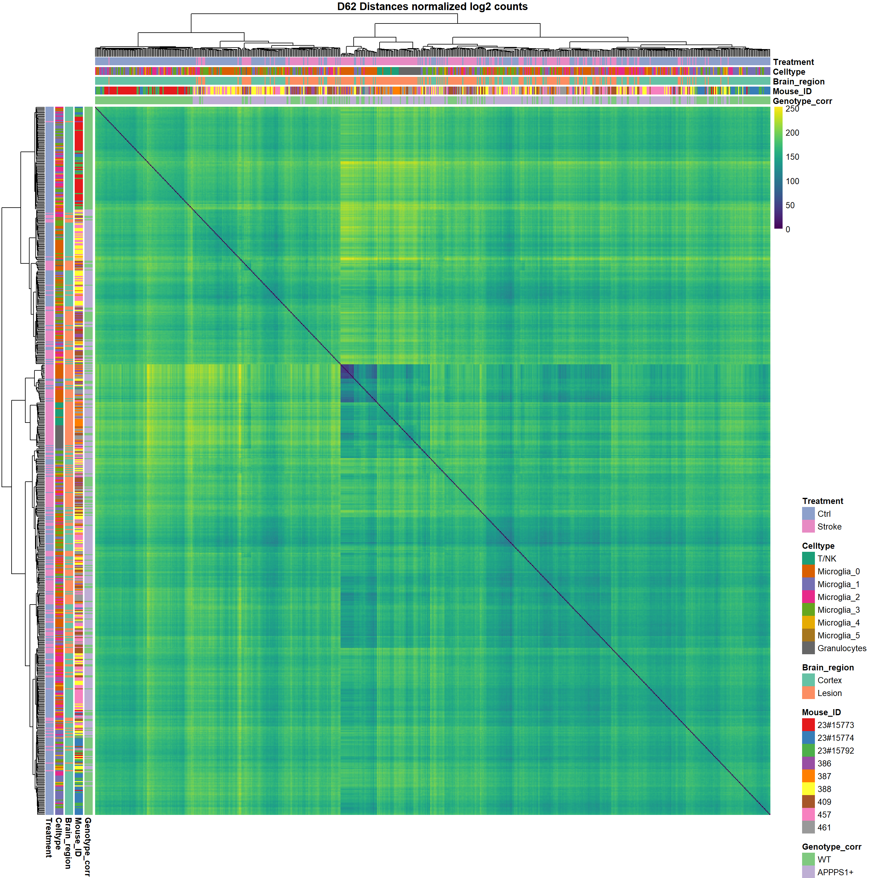
Genotype X Treatment Statistical modelling
getres=function(Celltype="Specify",
                Hypothesis="~1+Genotype_corr*Treatment",
                Target="Genotype_corrAPPPS1+:TreatmentStroke",
                Randomeffect="Sex"){

  res= comparison_rand(designform =Hypothesis,
                       randomeffect = Randomeffect,
                       Samples = samplemeta$Celltype==Celltype,
                       log_cpm = log2_cpm,
                       samplesdata = samplemeta,
                       target=Target)


  labels = samplemeta[samplemeta$Celltype==Celltype,c("Treatment", "Genotype_corr","Mouse_ID", "Brain_region", "Celltype")] %>%
    mutate_all(as.character) %>% as.data.frame()

  labels=labels %>% arrange(Treatment,Genotype_corr)
  plotdata=log2_cpm[res$adj.P.Val<0.05,rownames(labels)]

  pheatmap(plotdata,
           #clustering_method = "ward.D2",
           cluster_cols = F,
           cluster_rows  = T,
           scale ="column",
           show_rownames=F, show_colnames = F,
           legend=T,
           border_color = NA,
           #annotation_row = labels,
           annotation_col = labels,
           annotation_colors = ann_colors,
           col = colors,
           main = "D62 Distances normalized log2 counts")
  return(res)

}

generate_output=function(CT="Celltype", ...){
  respath=paste0(home, "/docs/LMER_",CT,".xlsx")

  analysis = getres(Celltype = CT)
  analysis_sig = analysis[analysis$adj.P.Val<0.05,]
  analysis_sig %>% display_tab()

  write.xlsx2(analysis_sig, file =respath , sheetName = "significant genes")

  ResGO = getGOresults(rownames(analysis_sig),
                       rownames(analysis),
                       "mmusculus")

  if(length(ResGO)>0){
    p=gostplot(ResGO)
  } else{
    ResGO=data.frame(result="no significant enrichment identified")
    p="no significant enrichment identified"
  }

  write.xlsx2(ResGO$result, file = respath, sheetName = "GO_enrichment", append=T)
  return(list(results=analysis,results_sig=analysis_sig, plot=p))
}
Microglia_0
res_output=generate_output("Microglia_0")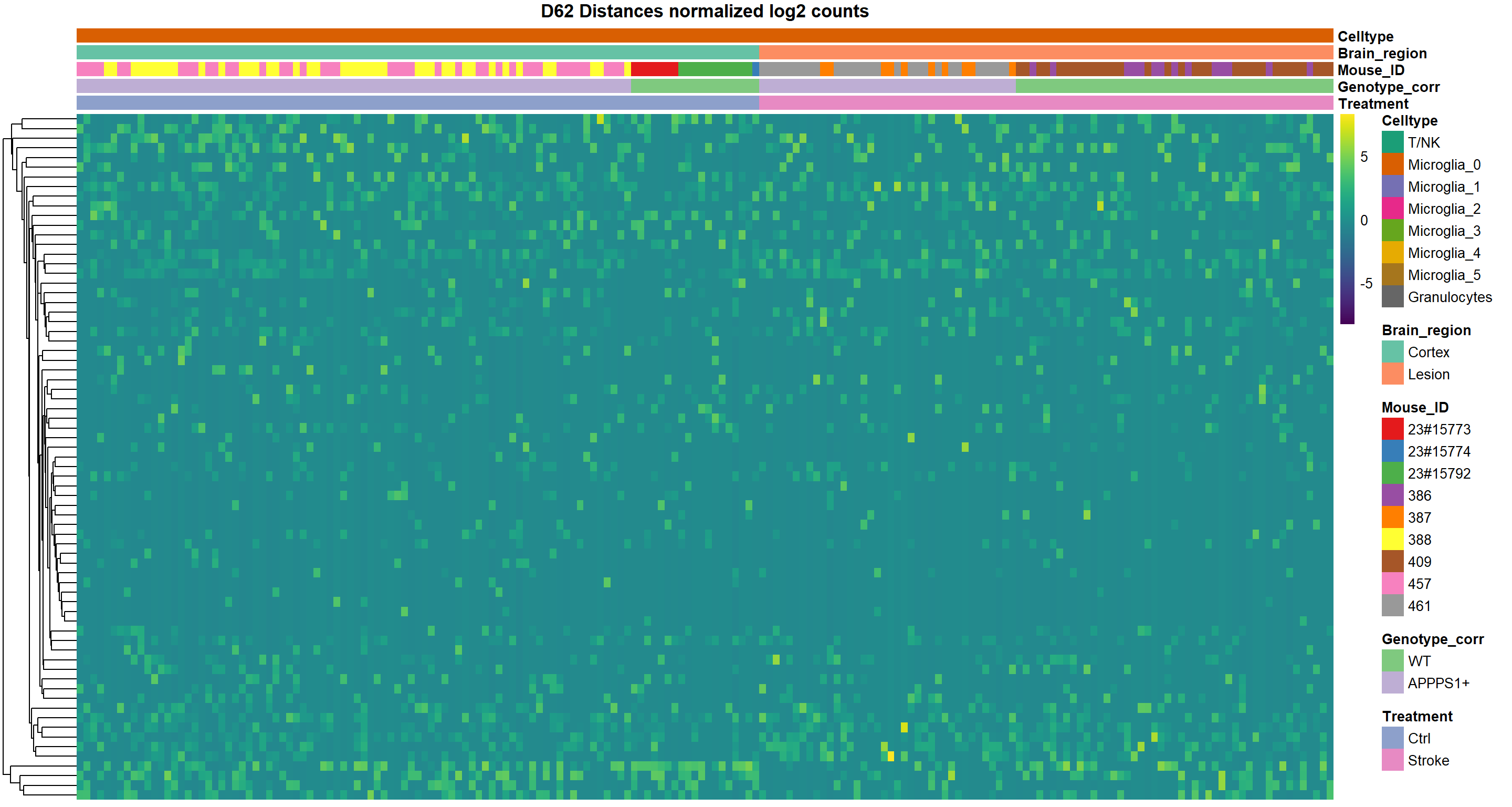
res_output[["results_sig"]] %>% display_tab()| logFC | AveExpr | t | P.Value | adj.P.Val | B | |
|---|---|---|---|---|---|---|
| Tbata | 3.522 | 0.454 | 14.822 | 0 | 0.000 | 60.871 |
| AC099934.1 | 2.090 | 0.223 | 13.572 | 0 | 0.000 | 53.259 |
| Rn7s1 | 4.868 | 0.932 | 13.345 | 0 | 0.000 | 51.865 |
| AY036118 | -9.974 | 6.541 | -10.095 | 0 | 0.000 | 31.986 |
| Prrx1 | 2.331 | 0.394 | 9.888 | 0 | 0.000 | 30.743 |
| Rn7s2 | 3.782 | 0.821 | 9.270 | 0 | 0.000 | 27.086 |
| Tmem170 | 2.199 | 0.349 | 9.155 | 0 | 0.000 | 26.415 |
| Mgmt | 2.584 | 0.444 | 7.476 | 0 | 0.000 | 16.971 |
| Lgals3bp | -7.696 | 3.952 | -6.731 | 0 | 0.000 | 13.081 |
| Olfr907 | 2.069 | 0.908 | 6.403 | 0 | 0.000 | 11.441 |
| Dock10 | 3.245 | 5.039 | 6.041 | 0 | 0.000 | 9.691 |
| Myl2 | 1.632 | 0.203 | 6.030 | 0 | 0.000 | 9.642 |
| Cd52 | -5.507 | 3.497 | -5.942 | 0 | 0.000 | 9.226 |
| Xist | 3.006 | 0.748 | 5.744 | 0 | 0.000 | 8.306 |
| Gm26870 | -3.903 | 9.134 | -5.639 | 0 | 0.000 | 7.830 |
| Fhl3 | 2.000 | 0.607 | 5.469 | 0 | 0.000 | 7.066 |
| Gm10076 | -3.831 | 2.856 | -5.441 | 0 | 0.000 | 6.942 |
| Pola2 | -2.445 | 2.264 | -5.344 | 0 | 0.000 | 6.519 |
| Lyz2 | -6.938 | 5.945 | -5.214 | 0 | 0.000 | 5.958 |
| Gm10719 | -3.401 | 6.711 | -5.214 | 0 | 0.000 | 5.957 |
| Upk1b | 3.244 | 1.015 | 5.173 | 0 | 0.000 | 5.782 |
| Gm15564 | 1.530 | 0.765 | 5.104 | 0 | 0.001 | 5.489 |
| Col6a3 | 2.052 | 0.420 | 5.023 | 0 | 0.001 | 5.150 |
| Apoe | -8.085 | 7.561 | -4.941 | 0 | 0.001 | 4.811 |
| Gnaz | 1.777 | 0.780 | 4.921 | 0 | 0.001 | 4.728 |
| D10Wsu102e | -1.853 | 7.009 | -4.852 | 0 | 0.001 | 4.445 |
| Gm26905 | -3.003 | 6.505 | -4.825 | 0 | 0.001 | 4.339 |
| Gm44215 | -3.369 | 3.605 | -4.801 | 0 | 0.002 | 4.240 |
| CT010467.1 | -3.433 | 10.638 | -4.709 | 0 | 0.002 | 3.873 |
| Gm11168 | -2.787 | 5.727 | -4.545 | 0 | 0.004 | 3.231 |
| Gm10722 | -2.870 | 5.562 | -4.538 | 0 | 0.004 | 3.202 |
| Gm10800 | -3.581 | 10.504 | -4.509 | 0 | 0.005 | 3.091 |
| Gm10717 | -2.839 | 6.955 | -4.471 | 0 | 0.006 | 2.948 |
| Traf2 | 2.132 | 0.995 | 4.467 | 0 | 0.006 | 2.929 |
| Gm37144 | 1.894 | 1.609 | 4.456 | 0 | 0.006 | 2.888 |
| Gm10801 | -3.026 | 7.744 | -4.421 | 0 | 0.006 | 2.758 |
| Soat1 | -3.263 | 2.004 | -4.355 | 0 | 0.008 | 2.510 |
| Cst7 | -5.555 | 3.339 | -4.335 | 0 | 0.009 | 2.434 |
| Gm20425 | 1.482 | 0.202 | 4.298 | 0 | 0.010 | 2.296 |
| Slc25a5 | -4.348 | 4.106 | -4.297 | 0 | 0.010 | 2.293 |
| Gm15500 | -4.193 | 4.285 | -4.281 | 0 | 0.010 | 2.235 |
| Gm14303 | -2.479 | 2.264 | -4.279 | 0 | 0.010 | 2.229 |
| Taf5l | 1.117 | 0.123 | 4.261 | 0 | 0.010 | 2.162 |
| Lipe | 1.932 | 1.789 | 4.255 | 0 | 0.010 | 2.140 |
| AW822252 | 1.266 | 0.732 | 4.211 | 0 | 0.012 | 1.980 |
| Nckap5l | 2.140 | 0.605 | 4.210 | 0 | 0.012 | 1.974 |
| Rbm15 | 2.276 | 0.888 | 4.191 | 0 | 0.012 | 1.905 |
| Ssr4 | -3.766 | 2.953 | -4.168 | 0 | 0.013 | 1.823 |
| Cyba | -3.637 | 5.245 | -4.157 | 0 | 0.014 | 1.783 |
| Gm43652 | 1.244 | 0.726 | 4.102 | 0 | 0.017 | 1.587 |
| Clec7a | -4.460 | 2.762 | -4.098 | 0 | 0.017 | 1.573 |
| Fmo1 | 1.488 | 0.512 | 4.060 | 0 | 0.019 | 1.439 |
| Fcer1g | -3.501 | 6.858 | -4.038 | 0 | 0.020 | 1.362 |
| Gm45220 | 2.414 | 0.695 | 4.036 | 0 | 0.020 | 1.354 |
| Tmem106c | 2.262 | 0.711 | 4.012 | 0 | 0.022 | 1.269 |
| Axl | -4.043 | 2.164 | -4.009 | 0 | 0.022 | 1.258 |
| Gm10443 | -2.528 | 2.200 | -4.003 | 0 | 0.022 | 1.238 |
| Polr3gl | 2.100 | 0.726 | 3.972 | 0 | 0.024 | 1.132 |
| Rpl13a | -3.451 | 4.835 | -3.960 | 0 | 0.025 | 1.090 |
| Ifi27l2a | -3.174 | 1.810 | -3.950 | 0 | 0.025 | 1.056 |
| B2m | -3.469 | 7.942 | -3.883 | 0 | 0.032 | 0.826 |
| Rps8 | -3.139 | 3.429 | -3.877 | 0 | 0.032 | 0.807 |
| Mzt2 | 1.955 | 0.682 | 3.796 | 0 | 0.043 | 0.533 |
| H2-K1 | -4.266 | 5.315 | -3.788 | 0 | 0.044 | 0.507 |
| Dnajc3 | -3.409 | 1.992 | -3.780 | 0 | 0.044 | 0.479 |
| Gm44645 | 1.097 | 0.462 | 3.770 | 0 | 0.045 | 0.447 |
| Lamp2 | -3.692 | 4.178 | -3.767 | 0 | 0.045 | 0.436 |
| Mtmr3 | 2.463 | 0.940 | 3.765 | 0 | 0.045 | 0.431 |
| Tsix | 1.075 | 0.243 | 3.753 | 0 | 0.046 | 0.392 |
| Eng | 2.294 | 0.862 | 3.742 | 0 | 0.047 | 0.355 |
| Rps21 | -2.554 | 2.191 | -3.735 | 0 | 0.048 | 0.331 |
res_output[["plot"]]get results table here
Microglia_1
res_output=generate_output("Microglia_1")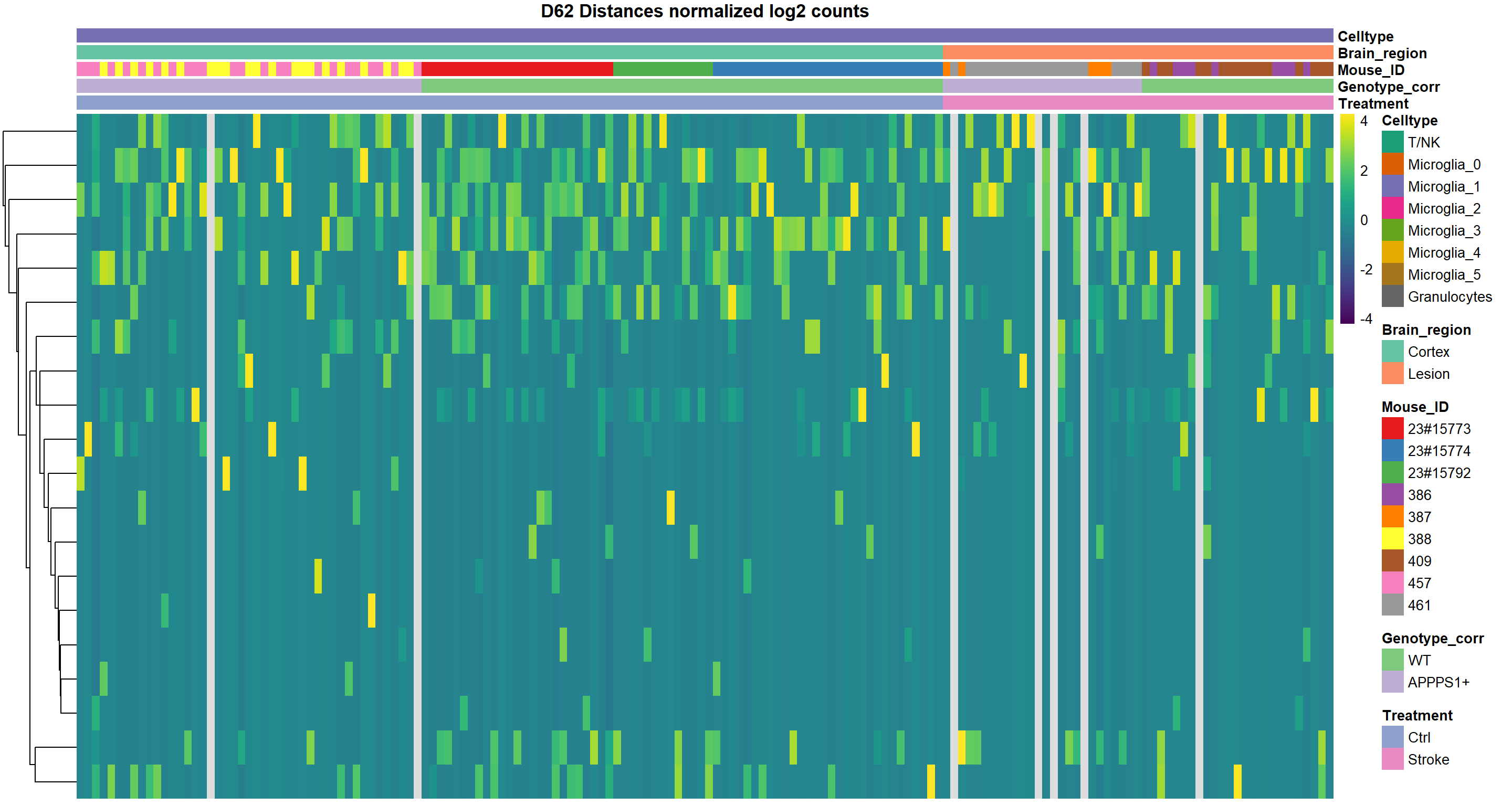
res_output[["results_sig"]] %>% display_tab()| logFC | AveExpr | t | P.Value | adj.P.Val | B | |
|---|---|---|---|---|---|---|
| Rn7s1 | 5.171 | 2.251 | 15.706 | 0 | 0.000 | 55.566 |
| AY036118 | -7.747 | 4.063 | -8.414 | 0 | 0.000 | 19.581 |
| Xist | 4.480 | 0.834 | 8.298 | 0 | 0.000 | 19.011 |
| Pola2 | -3.212 | 1.551 | -7.042 | 0 | 0.000 | 13.071 |
| Rn7s2 | 3.739 | 1.658 | 6.835 | 0 | 0.000 | 12.132 |
| AC099934.1 | 1.435 | 0.595 | 6.407 | 0 | 0.000 | 10.233 |
| Mgmt | 2.314 | 1.070 | 5.923 | 0 | 0.000 | 8.166 |
| Tsix | 2.028 | 0.342 | 5.846 | 0 | 0.000 | 7.844 |
| Tbata | 1.984 | 1.018 | 4.947 | 0 | 0.003 | 4.306 |
| Tmem170 | 2.015 | 1.087 | 4.917 | 0 | 0.003 | 4.196 |
| Gm26870 | -4.250 | 2.611 | -4.821 | 0 | 0.004 | 3.845 |
| Zfp992 | -2.797 | 0.847 | -4.604 | 0 | 0.010 | 3.065 |
| Gm10719 | -3.041 | 1.702 | -4.520 | 0 | 0.012 | 2.771 |
| Gm15564 | 1.545 | 1.085 | 4.493 | 0 | 0.013 | 2.678 |
| Gm10801 | -3.336 | 1.981 | -4.468 | 0 | 0.013 | 2.591 |
| Gm10800 | -4.381 | 3.697 | -4.258 | 0 | 0.030 | 1.878 |
| Gm10722 | -2.146 | 0.803 | -4.174 | 0 | 0.039 | 1.603 |
| Cst7 | -4.417 | 1.822 | -4.162 | 0 | 0.039 | 1.563 |
| Slc6a20b | 1.468 | 0.968 | 4.101 | 0 | 0.046 | 1.366 |
| Gm26822 | 1.544 | 1.578 | 4.092 | 0 | 0.046 | 1.336 |
res_output[["plot"]]get results table here
Microglia_2
res_output=generate_output("Microglia_2")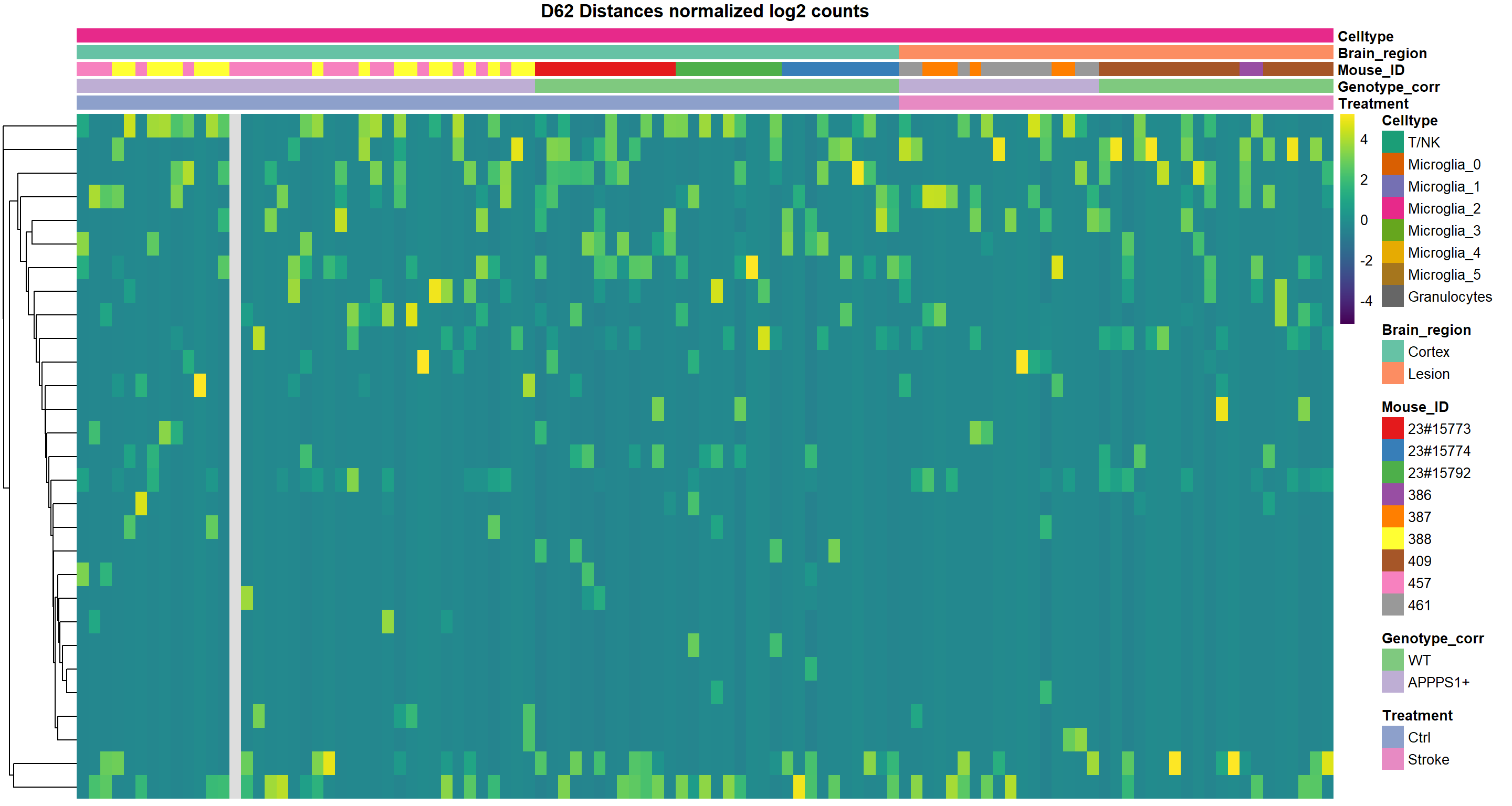
res_output[["results_sig"]] %>% display_tab()| logFC | AveExpr | t | P.Value | adj.P.Val | B | |
|---|---|---|---|---|---|---|
| AY036118 | -10.106 | 5.877 | -13.790 | 0 | 0.000 | 40.529 |
| AC099934.1 | 2.240 | 0.649 | 13.121 | 0 | 0.000 | 37.942 |
| Rn7s1 | 5.881 | 2.015 | 12.703 | 0 | 0.000 | 36.288 |
| Tbata | 3.400 | 1.094 | 9.836 | 0 | 0.000 | 24.360 |
| Tmem170 | 2.548 | 0.931 | 8.343 | 0 | 0.000 | 17.927 |
| Mgmt | 3.287 | 1.015 | 8.171 | 0 | 0.000 | 17.183 |
| Gab3 | 4.652 | 1.369 | 7.325 | 0 | 0.000 | 13.580 |
| Gm10719 | -5.301 | 4.443 | -7.065 | 0 | 0.000 | 12.488 |
| Gm26870 | -6.685 | 6.156 | -6.989 | 0 | 0.000 | 12.169 |
| Gm10800 | -6.887 | 7.447 | -6.841 | 0 | 0.000 | 11.553 |
| Gm15564 | 2.706 | 1.222 | 6.700 | 0 | 0.000 | 10.972 |
| Gm10801 | -5.372 | 5.022 | -6.609 | 0 | 0.000 | 10.599 |
| Gm10717 | -4.477 | 4.416 | -6.084 | 0 | 0.000 | 8.477 |
| Prrx1 | 1.709 | 0.589 | 5.548 | 0 | 0.000 | 6.389 |
| Rn7s2 | 3.611 | 1.358 | 5.396 | 0 | 0.000 | 5.817 |
| Gm37716 | 1.631 | 0.489 | 4.840 | 0 | 0.004 | 3.786 |
| Xist | 3.446 | 0.711 | 4.830 | 0 | 0.004 | 3.750 |
| Pola2 | -2.603 | 2.295 | -4.758 | 0 | 0.005 | 3.499 |
| CT010467.1 | -1.778 | 11.024 | -4.746 | 0 | 0.005 | 3.456 |
| Gm11168 | -3.190 | 3.320 | -4.726 | 0 | 0.005 | 3.386 |
| A430010J10Rik | 1.554 | 1.105 | 4.427 | 0 | 0.015 | 2.363 |
| Gm44068 | -1.496 | 0.544 | -4.406 | 0 | 0.016 | 2.294 |
| Gm28661 | -5.071 | 4.633 | -4.295 | 0 | 0.023 | 1.928 |
| Gm22567 | 1.380 | 0.525 | 4.222 | 0 | 0.029 | 1.689 |
| AC127302.1 | -2.557 | 3.170 | -4.213 | 0 | 0.029 | 1.659 |
| Gm21738 | -3.628 | 3.300 | -4.176 | 0 | 0.032 | 1.539 |
| Rpl19-ps11 | -1.655 | 0.404 | -4.115 | 0 | 0.039 | 1.345 |
| Gm10359 | 2.833 | 1.183 | 4.036 | 0 | 0.049 | 1.094 |
| Gm12671 | 2.833 | 1.183 | 4.036 | 0 | 0.049 | 1.094 |
res_output[["plot"]]get results table here
Microglia_3
res_output=generate_output("Microglia_3")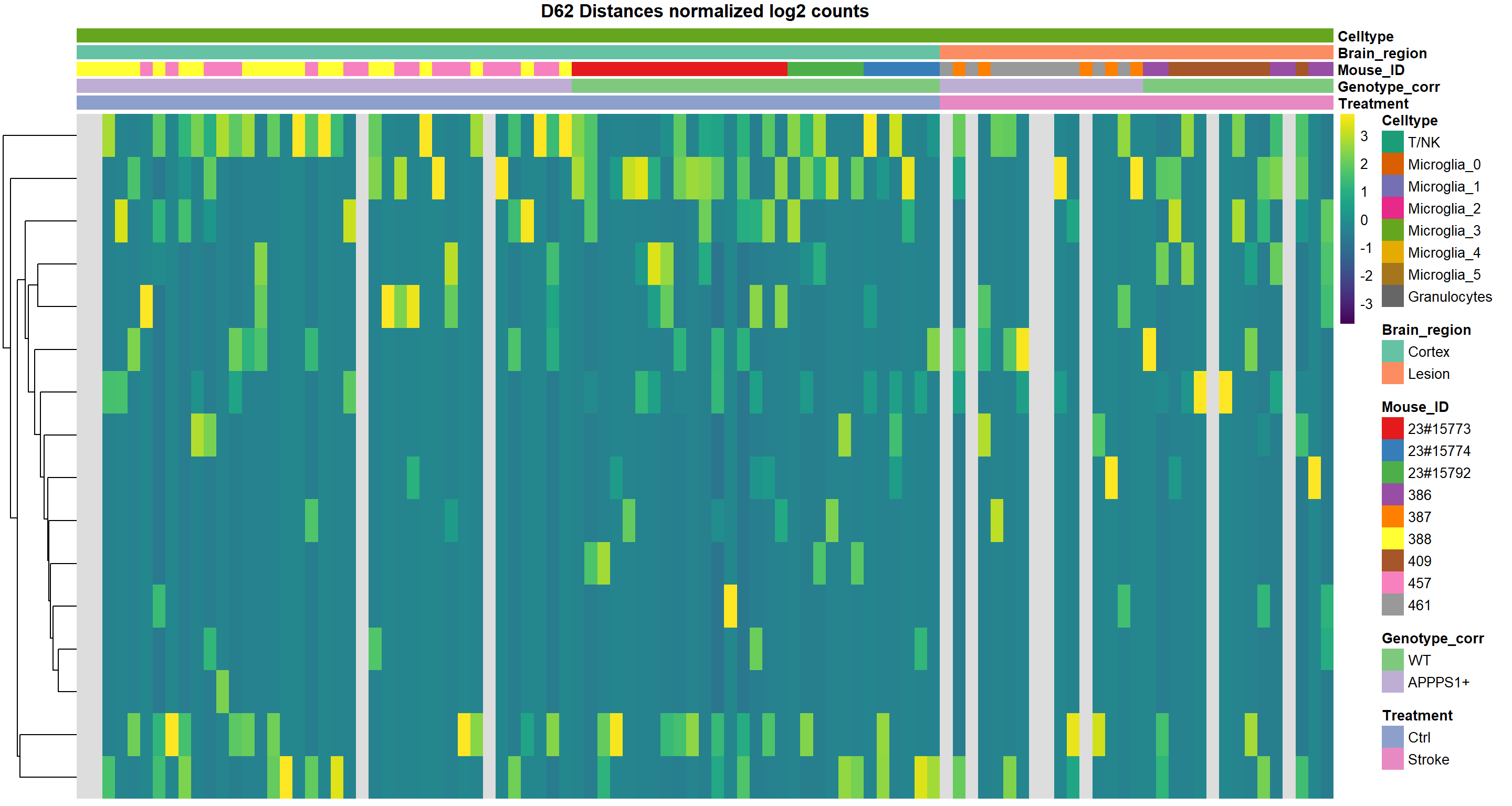
[1] "no significant GO terms identified"res_output[["results_sig"]] %>% display_tab()| logFC | AveExpr | t | P.Value | adj.P.Val | B | |
|---|---|---|---|---|---|---|
| Apoe | -10.329 | 8.936 | -11.161 | 0 | 0.000 | 27.508 |
| Rn7s1 | 4.871 | 1.890 | 10.710 | 0 | 0.000 | 25.819 |
| Tmem170 | 2.313 | 0.742 | 9.944 | 0 | 0.000 | 22.898 |
| AY036118 | -8.824 | 5.396 | -6.850 | 0 | 0.000 | 10.815 |
| Tbata | 2.553 | 0.831 | 6.560 | 0 | 0.000 | 9.704 |
| Cst7 | -6.295 | 5.374 | -5.748 | 0 | 0.000 | 6.680 |
| Rn7s2 | 3.502 | 1.489 | 5.388 | 0 | 0.001 | 5.390 |
| Mgmt | 2.551 | 0.931 | 5.248 | 0 | 0.002 | 4.901 |
| Gm15564 | 2.059 | 1.137 | 5.108 | 0 | 0.002 | 4.415 |
| Lyz2 | -4.371 | 7.997 | -5.064 | 0 | 0.003 | 4.264 |
| Xist | 3.215 | 0.580 | 5.053 | 0 | 0.003 | 4.228 |
| AC099934.1 | 1.361 | 0.399 | 4.751 | 0 | 0.008 | 3.211 |
| Ctsb | -2.050 | 9.953 | -4.472 | 0 | 0.022 | 2.301 |
| Prrx1 | 1.217 | 0.338 | 4.398 | 0 | 0.027 | 2.068 |
| Clec7a | -5.414 | 3.980 | -4.293 | 0 | 0.038 | 1.736 |
| Slc25a37 | 3.907 | 1.361 | 4.258 | 0 | 0.041 | 1.628 |
res_output[["plot"]][1] "no significant enrichment identified"get results table here
Microglia_4
calculation not converging as Celltype not identified in all conditions however also rare in other conditions, no significant difference
idx=samplemeta$Celltype=="Microglia_4"
table(samplemeta$Treatment[idx], samplemeta$Genotype_corr[idx])
         WT APPPS1+
  Ctrl   11      10
  Stroke  4       1
table(samplemeta$Treatment[idx], samplemeta$Genotype_corr[idx]) %>% fisher.test()
    Fisher's Exact Test for Count Data

data:  .
p-value = 0.3562
alternative hypothesis: true odds ratio is not equal to 1
95 percent confidence interval:
 0.005090941 3.588141911
sample estimates:
odds ratio
 0.2877466
#res_output=generate_output("Microglia_4")
#res_output[["results_sig"]] %>% display_tab()
#res_output[["plot"]]get results table here
Microglia_5
res_output=generate_output("Microglia_5")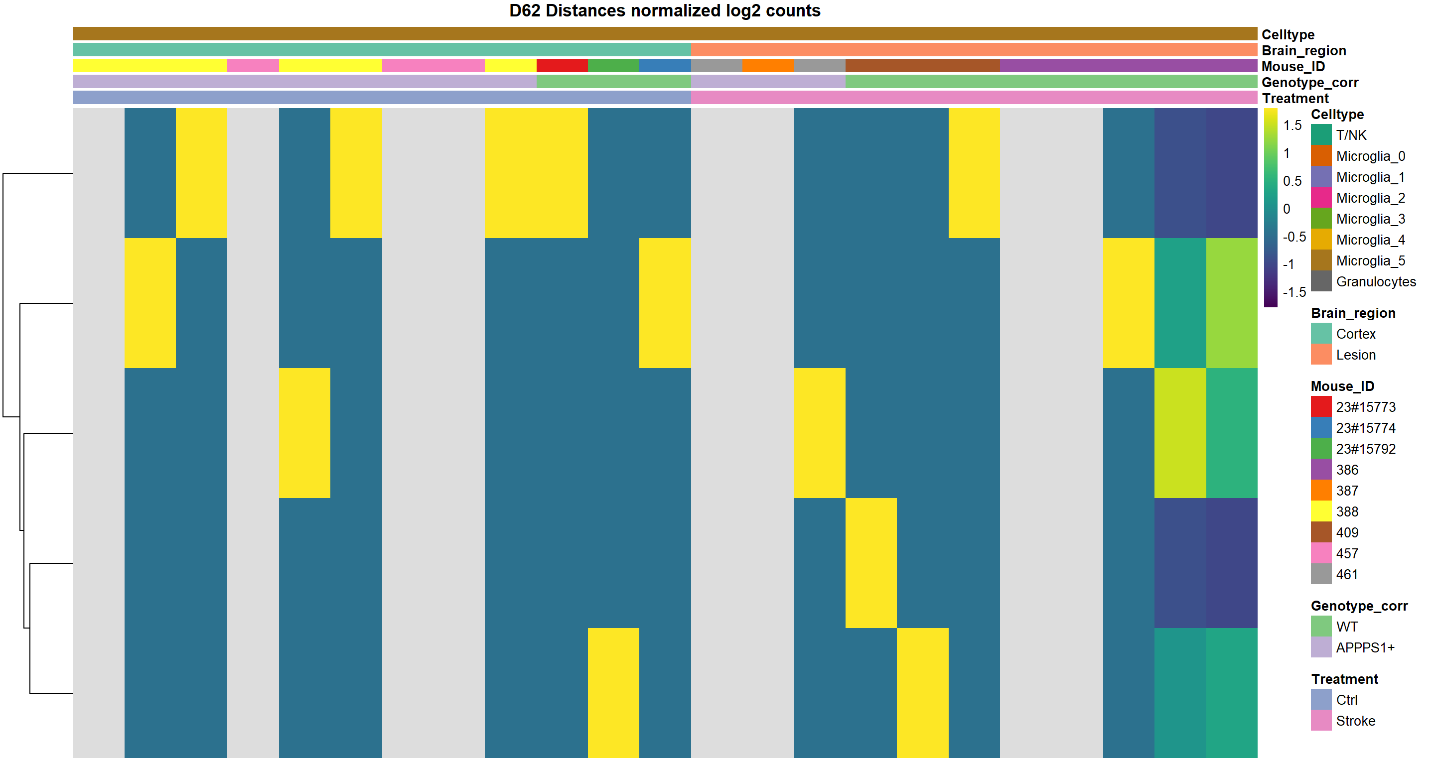
[1] "no significant GO terms identified"res_output[["results_sig"]] %>% display_tab()| logFC | AveExpr | t | P.Value | adj.P.Val | B | |
|---|---|---|---|---|---|---|
| Strip1 | 5.337 | 0.696 | 15.181 | 0 | 0.000 | 10.786 |
| Naalad2 | 6.931 | 0.908 | 12.659 | 0 | 0.000 | 9.531 |
| Ino80 | 5.064 | 0.811 | 9.524 | 0 | 0.000 | 7.170 |
| AC131743.1 | 1.546 | 0.200 | 7.232 | 0 | 0.002 | 4.604 |
| Slc2a3 | 1.734 | 0.289 | 6.052 | 0 | 0.019 | 2.928 |
res_output[["plot"]][1] "no significant enrichment identified"get results table here
Granulozytes
calculation not converging as Celltype not identified in all conditions however also rare in other conditions, no significant difference
idx=samplemeta$Celltype=="Granulocytes"
table(samplemeta$Treatment[idx], samplemeta$Genotype_corr[idx])
         WT APPPS1+
  Ctrl    0       2
  Stroke  6      14
table(samplemeta$Treatment[idx], samplemeta$Genotype_corr[idx]) %>% fisher.test()
    Fisher's Exact Test for Count Data

data:  .
p-value = 1
alternative hypothesis: true odds ratio is not equal to 1
95 percent confidence interval:
  0.0000 14.7518
sample estimates:
odds ratio
         0
# res_output=generate_output("Granulocytes ")
# res_output[["results_sig"]] %>% display_tab()
# res_output[["plot"]]get results table here
T_NK
idx=samplemeta$Celltype=="T/NK"
table(samplemeta$Treatment[idx], samplemeta$Genotype_corr[idx])
         WT APPPS1+
  Ctrl    1       2
  Stroke  2      17
table(samplemeta$Treatment[idx], samplemeta$Genotype_corr[idx]) %>% fisher.test()
    Fisher's Exact Test for Count Data

data:  .
p-value = 0.3708
alternative hypothesis: true odds ratio is not equal to 1
95 percent confidence interval:
   0.0481749 117.2316789
sample estimates:
odds ratio
  3.869104
# res_output=generate_output("T/NK")
# res_output[["results_sig"]] %>% display_tab()
# res_output[["plot"]]get results table here
Gene expression plot
sessionInfo()R version 4.1.2 (2021-11-01)
Platform: x86_64-w64-mingw32/x64 (64-bit)
Running under: Windows 10 x64 (build 18363)
Matrix products: default
locale:
[1] LC_COLLATE=German_Germany.1252 LC_CTYPE=German_Germany.1252 LC_MONETARY=German_Germany.1252 LC_NUMERIC=C LC_TIME=German_Germany.1252
attached base packages:
[1] stats4 stats graphics grDevices utils datasets methods base
other attached packages:
[1] gprofiler2_0.2.1 lm.beta_1.5-1 pheatmap_1.0.12 RColorBrewer_1.1-2 kableExtra_1.3.4 viridis_0.6.2 viridisLite_0.4.0 xlsx_0.6.5 brms_2.16.3 Rcpp_1.0.8 compareGroups_4.5.1 data.table_1.14.2 SingleR_1.8.1 SeuratObject_4.0.4 Seurat_4.1.0 forcats_0.5.1 stringr_1.4.0 dplyr_1.0.7 purrr_0.3.4 readr_2.1.2 tidyr_1.1.4 tibble_3.1.6 ggplot2_3.3.5 tidyverse_1.3.1 DESeq2_1.34.0 SummarizedExperiment_1.24.0 Biobase_2.54.0 MatrixGenerics_1.6.0 matrixStats_0.61.0 GenomicRanges_1.46.1 GenomeInfoDb_1.30.1 IRanges_2.28.0 S4Vectors_0.32.3 BiocGenerics_0.40.0 limma_3.50.0 workflowr_1.7.0
loaded via a namespace (and not attached):
[1] scattermore_0.7 coda_0.19-4 bit64_4.0.5 knitr_1.37 dygraphs_1.1.1.6 irlba_2.3.5 DelayedArray_0.20.0 inline_0.3.19 rpart_4.1.16 KEGGREST_1.34.0 RCurl_1.98-1.5 generics_0.1.2 ScaledMatrix_1.2.0 callr_3.7.0 cowplot_1.1.1 RSQLite_2.2.9 mice_3.14.0 RANN_2.6.1 future_1.23.0 chron_2.3-56 bit_4.0.4 tzdb_0.2.0 spatstat.data_2.1-2 webshot_0.5.2 xml2_1.3.3 lubridate_1.8.0 httpuv_1.6.5 StanHeaders_2.21.0-7 assertthat_0.2.1 xfun_0.29 rJava_1.0-6 hms_1.1.1 jquerylib_0.1.4 bayesplot_1.8.1 evaluate_0.14 promises_1.2.0.1 fansi_1.0.2 dbplyr_2.1.1 readxl_1.3.1 igraph_1.2.11 DBI_1.1.2 geneplotter_1.72.0 Rsolnp_1.16 htmlwidgets_1.5.4 tensorA_0.36.2 spatstat.geom_2.3-1 ellipsis_0.3.2 crosstalk_1.2.0 backports_1.4.1 markdown_1.1 annotate_1.72.0 RcppParallel_5.1.5 deldir_1.0-6 sparseMatrixStats_1.6.0 vctrs_0.3.8 ROCR_1.0-11 abind_1.4-5 cachem_1.0.6 withr_2.4.3 packrat_0.7.0 HardyWeinberg_1.7.4 checkmate_2.0.0 sctransform_0.3.3 prettyunits_1.1.1 xts_0.12.1 goftest_1.2-3 svglite_2.0.0 cluster_2.1.2 lazyeval_0.2.2 crayon_1.4.2 genefilter_1.76.0 pkgconfig_2.0.3 nlme_3.1-155 nnet_7.3-17 rlang_1.0.0 globals_0.14.0 lifecycle_1.0.1 miniUI_0.1.1.1 colourpicker_1.1.1 modelr_0.1.8 rsvd_1.0.5 distributional_0.3.0 cellranger_1.1.0 rprojroot_2.0.2 polyclip_1.10-0 lmtest_0.9-39 flextable_0.6.10 Matrix_1.4-0 loo_2.4.1 zoo_1.8-9 reprex_2.0.1 base64enc_0.1-3 whisker_0.4 ggridges_0.5.3 processx_3.5.2 png_0.1-7 bitops_1.0-7 getPass_0.2-2 KernSmooth_2.23-20 Biostrings_2.62.0 blob_1.2.2 DelayedMatrixStats_1.16.0 parallelly_1.30.0 shinystan_2.5.0 beachmat_2.10.0 scales_1.1.1 memoise_2.0.1 magrittr_2.0.2 plyr_1.8.6 ica_1.0-2 threejs_0.3.3 zlibbioc_1.40.0 compiler_4.1.2 rstantools_2.1.1 fitdistrplus_1.1-6 cli_3.1.1 XVector_0.34.0 listenv_0.8.0 Brobdingnag_1.2-7 patchwork_1.1.1 pbapply_1.5-0 ps_1.6.0 MASS_7.3-55 mgcv_1.8-38 tidyselect_1.1.1 stringi_1.7.6 highr_0.9 yaml_2.2.2 askpass_1.1 BiocSingular_1.10.0 locfit_1.5-9.4 ggrepel_0.9.1 bridgesampling_1.1-2 grid_4.1.2 sass_0.4.0 tools_4.1.2 future.apply_1.8.1 parallel_4.1.2 rstudioapi_0.13 uuid_1.0-3 git2r_0.29.0 gridExtra_2.3 farver_2.1.0 posterior_1.2.0 Rtsne_0.15 BiocManager_1.30.16 digest_0.6.29 shiny_1.7.1 broom_0.7.12 later_1.3.0 writexl_1.4.0 RcppAnnoy_0.0.19 httr_1.4.2 gdtools_0.2.3 AnnotationDbi_1.56.2 rsconnect_0.8.25 colorspace_2.0-2 rvest_1.0.2 XML_3.99-0.8 fs_1.5.2 tensor_1.5 reticulate_1.24 truncnorm_1.0-8 splines_4.1.2 statmod_1.4.36 uwot_0.1.11 spatstat.utils_2.3-0 xlsxjars_0.6.1 shinythemes_1.2.0 plotly_4.10.0 systemfonts_1.0.3 xtable_1.8-4 jsonlite_1.7.3 rstan_2.21.3 R6_2.5.1 pillar_1.7.0 htmltools_0.5.2 mime_0.12 DT_0.20 glue_1.6.1 fastmap_1.1.0 BiocParallel_1.28.3 BiocNeighbors_1.12.0 codetools_0.2-18 pkgbuild_1.3.1 mvtnorm_1.1-3 utf8_1.2.2 lattice_0.20-45 bslib_0.3.1 spatstat.sparse_2.1-0 curl_4.3.2 leiden_0.3.9 gtools_3.9.2 officer_0.4.1 openssl_1.4.6 shinyjs_2.1.0 zip_2.2.0 survival_3.2-13 rmarkdown_2.11 munsell_0.5.0 GenomeInfoDbData_1.2.7 haven_2.4.3 reshape2_1.4.4 gtable_0.3.0 spatstat.core_2.3-2