Investigate V after every iteration in SuSiE RSS
Dat Do
2025-09-08
Last updated: 2025-09-08
Checks: 6 1
Knit directory: Improved_LD_SuSiE/
This reproducible R Markdown analysis was created with workflowr (version 1.7.1). The Checks tab describes the reproducibility checks that were applied when the results were created. The Past versions tab lists the development history.
Great! Since the R Markdown file has been committed to the Git repository, you know the exact version of the code that produced these results.
Great job! The global environment was empty. Objects defined in the global environment can affect the analysis in your R Markdown file in unknown ways. For reproduciblity it’s best to always run the code in an empty environment.
The command set.seed(20250821) was run prior to running
the code in the R Markdown file. Setting a seed ensures that any results
that rely on randomness, e.g. subsampling or permutations, are
reproducible.
Great job! Recording the operating system, R version, and package versions is critical for reproducibility.
Nice! There were no cached chunks for this analysis, so you can be confident that you successfully produced the results during this run.
Using absolute paths to the files within your workflowr project makes it difficult for you and others to run your code on a different machine. Change the absolute path(s) below to the suggested relative path(s) to make your code more reproducible.
| absolute | relative |
|---|---|
| ~/Documents/Improved_LD_SuSiE | . |
Great! You are using Git for version control. Tracking code development and connecting the code version to the results is critical for reproducibility.
The results in this page were generated with repository version 0e1cebc. See the Past versions tab to see a history of the changes made to the R Markdown and HTML files.
Note that you need to be careful to ensure that all relevant files for
the analysis have been committed to Git prior to generating the results
(you can use wflow_publish or
wflow_git_commit). workflowr only checks the R Markdown
file, but you know if there are other scripts or data files that it
depends on. Below is the status of the Git repository when the results
were generated:
Ignored files:
    Ignored:    .DS_Store
    Ignored:    .Rhistory
    Ignored:    .Rproj.user/
    Ignored:    analysis/.Rhistory
    Ignored:    code/.DS_Store

Untracked files:
    Untracked:  code/R_algorithms.R
    Untracked:  code/SuSiE_rss.R
    Untracked:  code/SuSiE_rss_multi_SNPs.R
    Untracked:  code/SuSiE_rss_test.R
    Untracked:  code/compare_LD_mat_Dykstra_fullSVD.R
    Untracked:  code/prototype_R_code.R
    Untracked:  code/test_visualize_many_traits.R
    Untracked:  code/test_visualize_one_trait.R
    Untracked:  code_push.R
    Untracked:  output/coverages_mat_multi_trait.RData
    Untracked:  output/number_CSs_mat_multi_trait.RData
    Untracked:  output/number_SNPs_per_CS_mat_multi_trait.RData
    Untracked:  output/powers_mat_multi_trait.RData
Note that any generated files, e.g. HTML, png, CSS, etc., are not included in this status report because it is ok for generated content to have uncommitted changes.
These are the previous versions of the repository in which changes were
made to the R Markdown (analysis/V_xy_iter_investigate.Rmd)
and HTML (docs/V_xy_iter_investigate.html) files. If you’ve
configured a remote Git repository (see ?wflow_git_remote),
click on the hyperlinks in the table below to view the files as they
were in that past version.
| File | Version | Author | Date | Message |
|---|---|---|---|---|
| Rmd | 0e1cebc | dodat97 | 2025-09-08 | wflow_publish(c("analysis/V_xy_iter_investigate.Rmd")) |
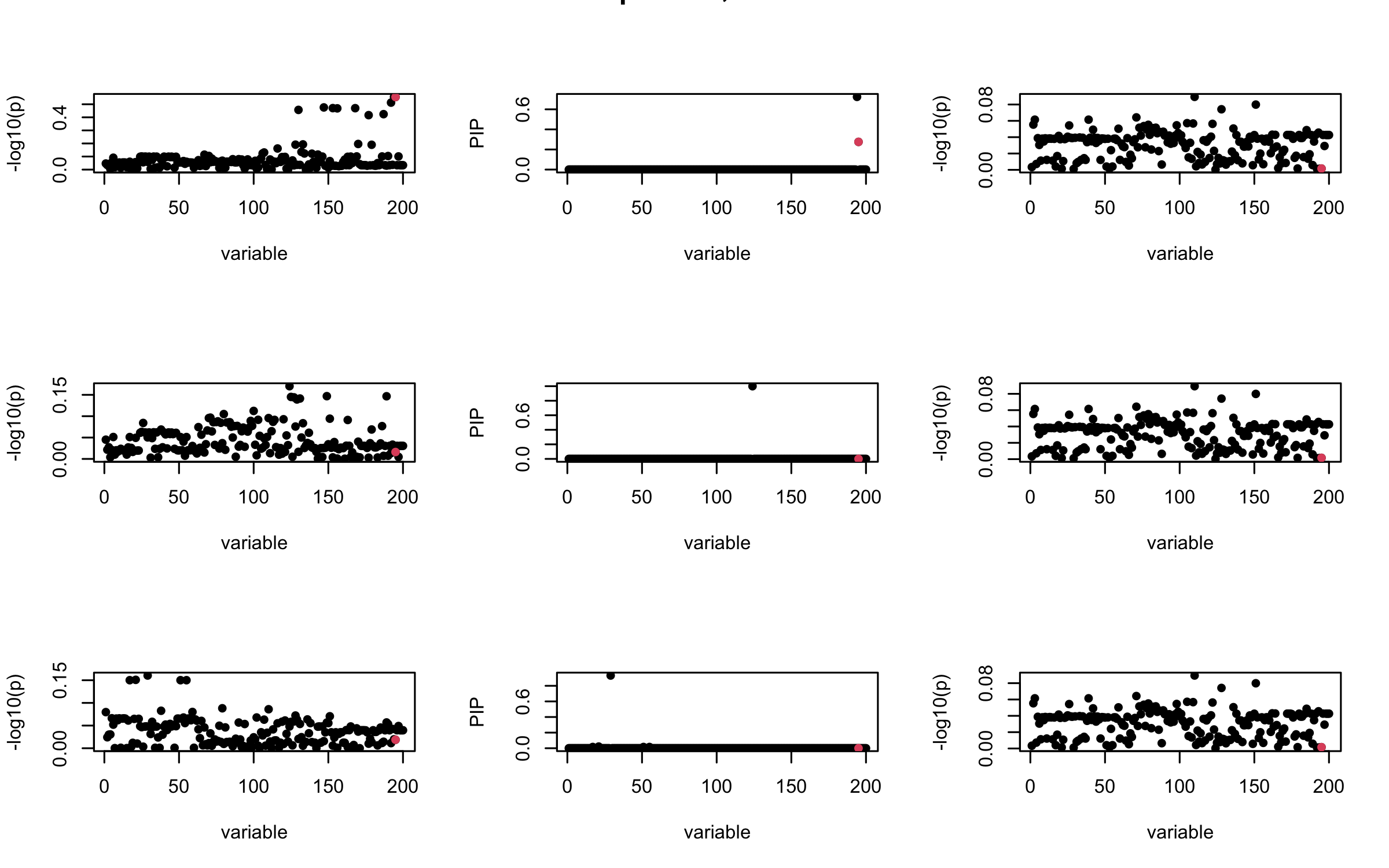
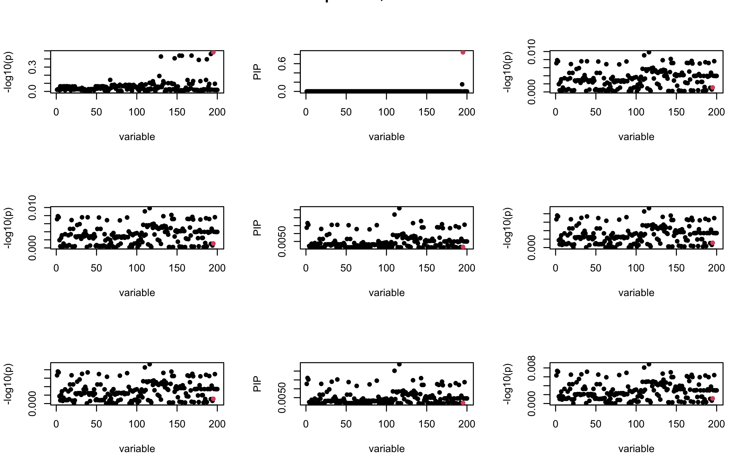
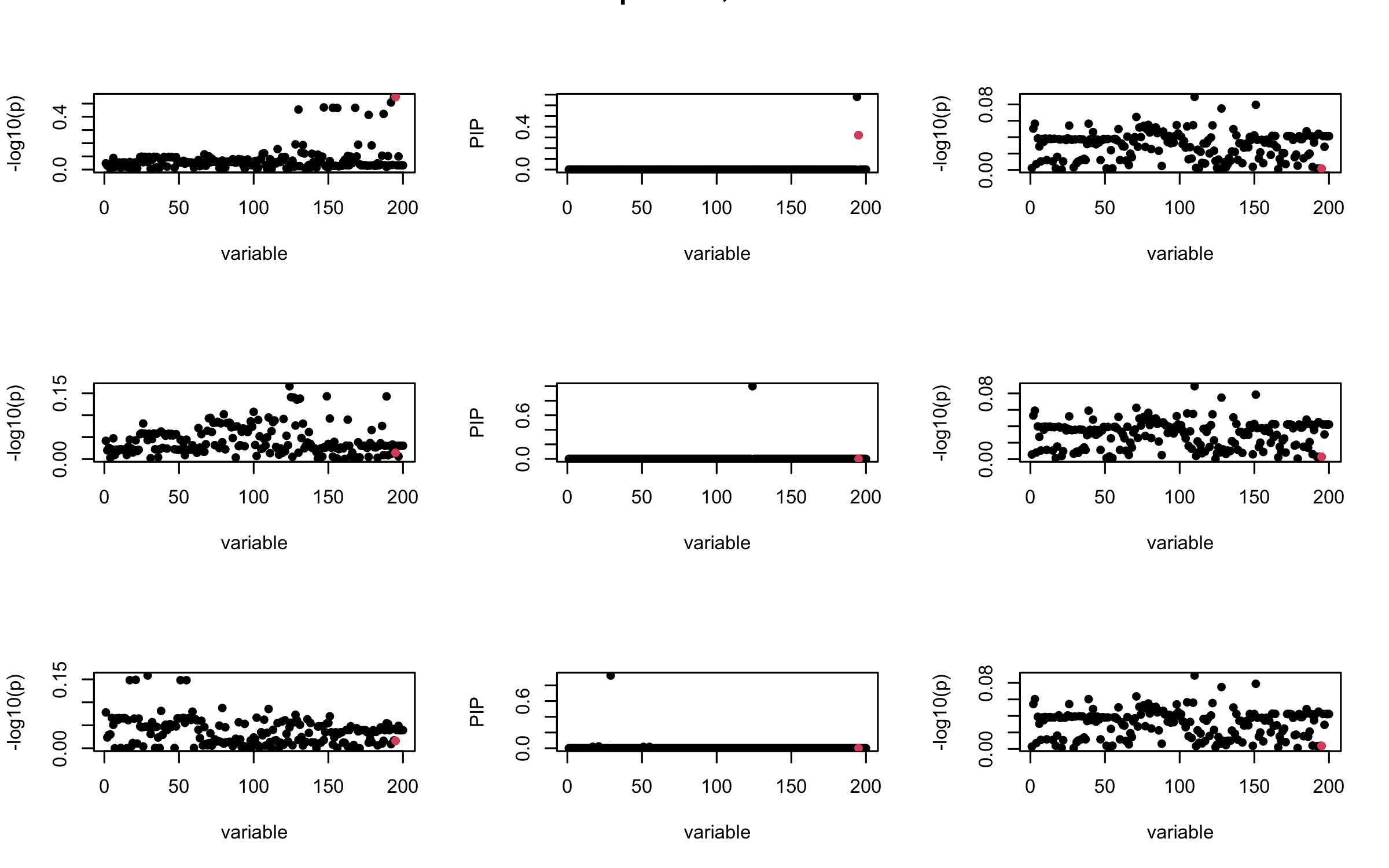
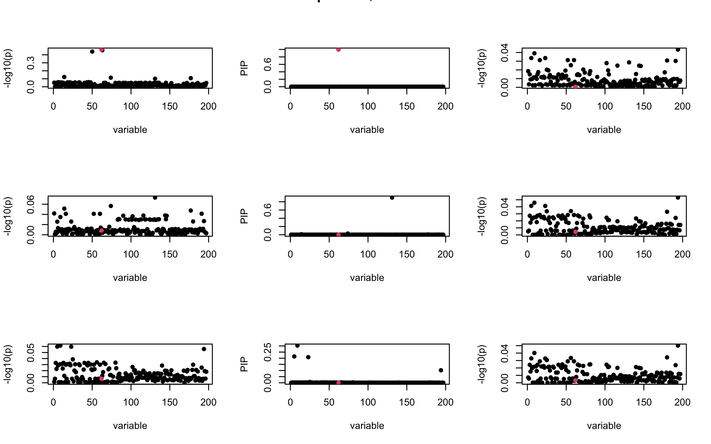
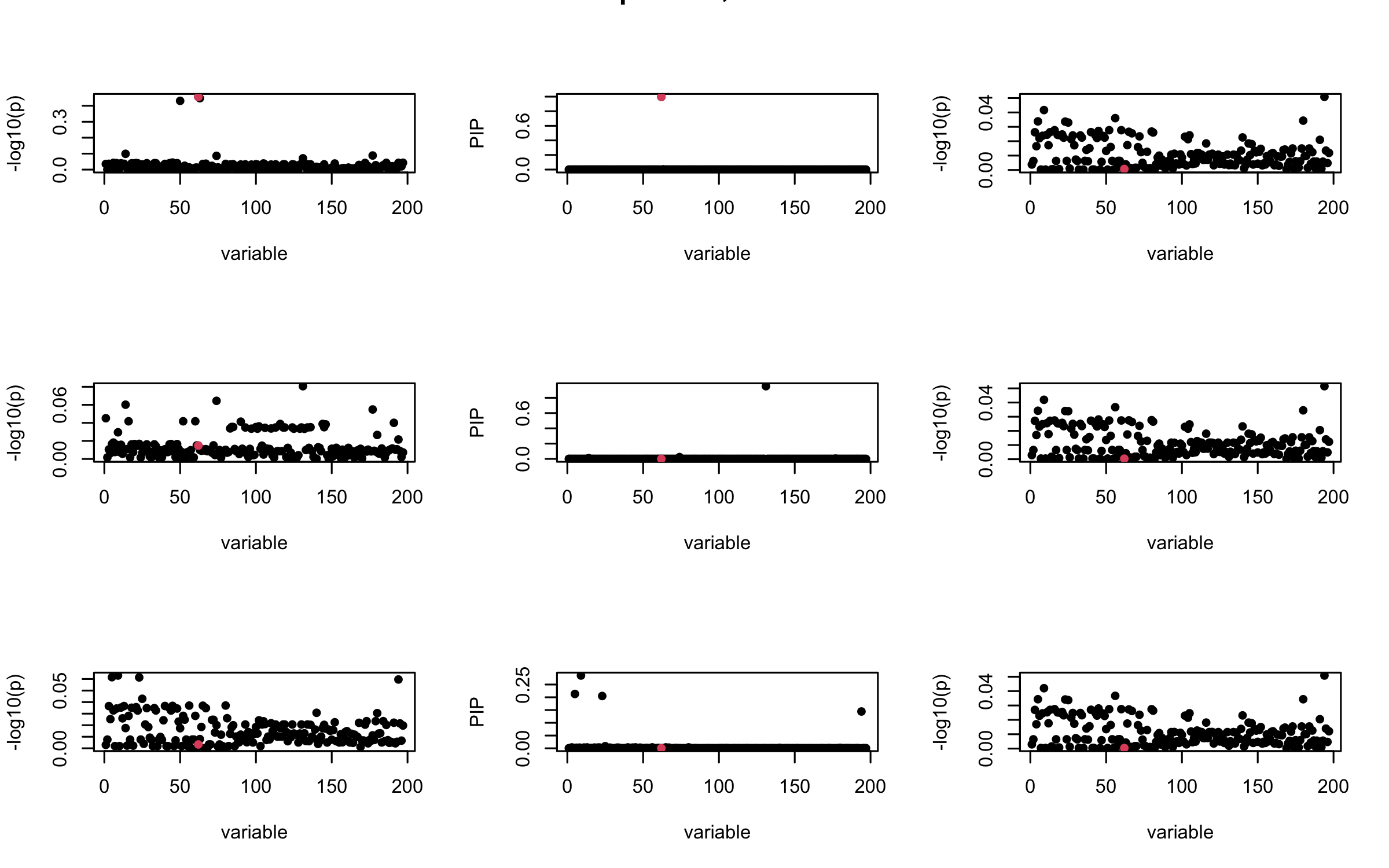
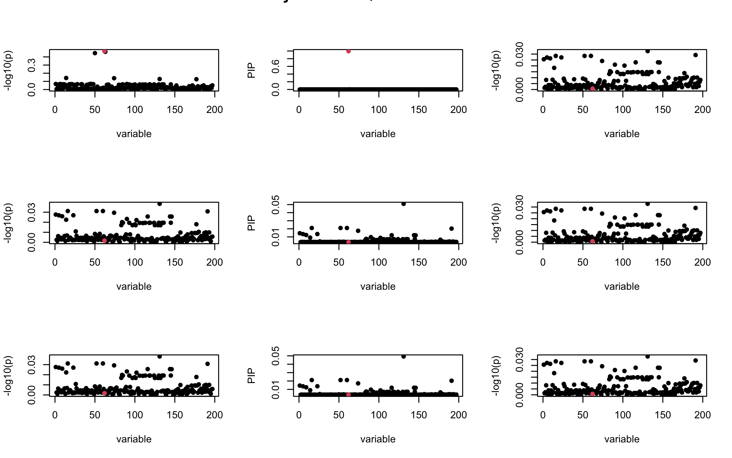
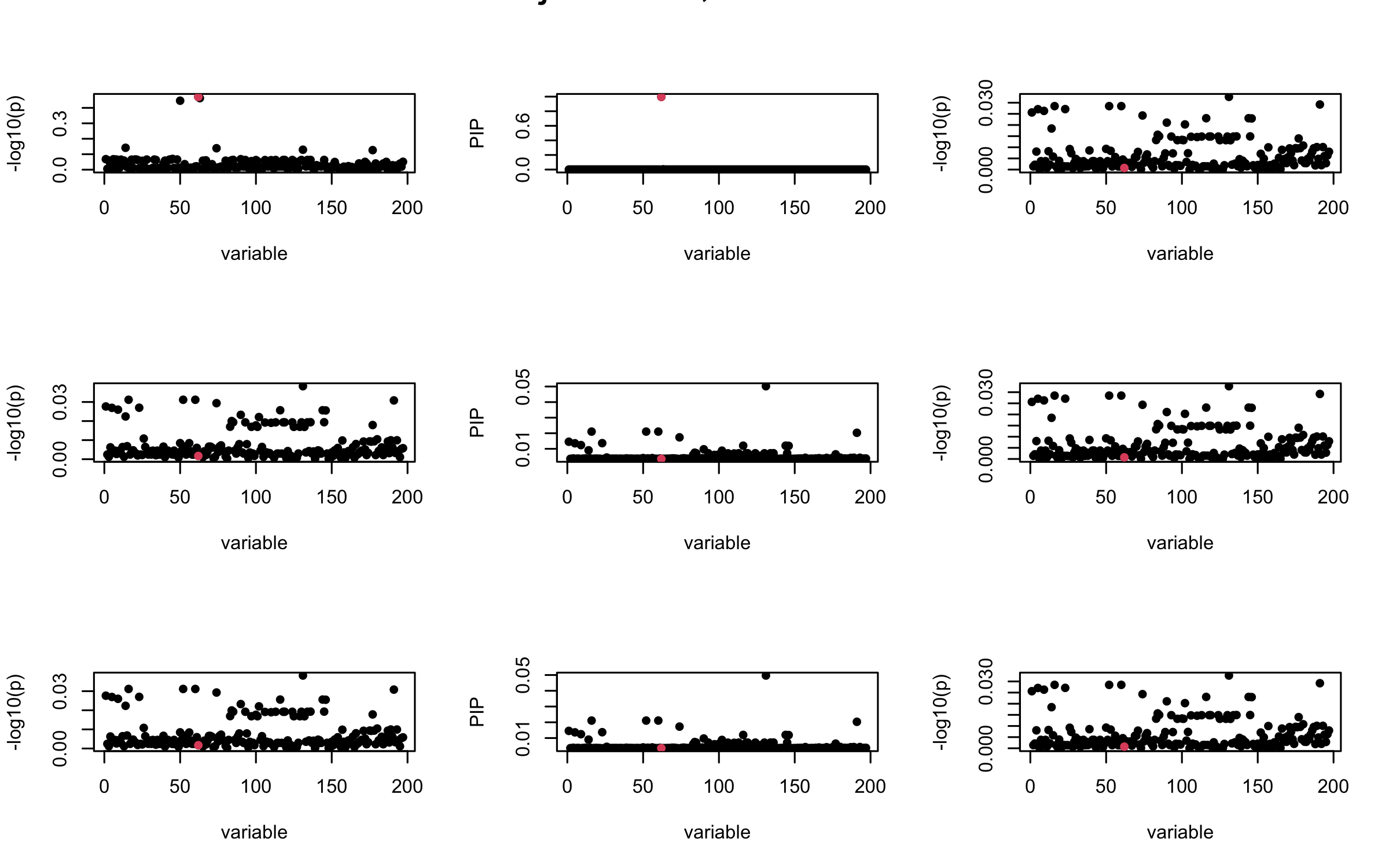
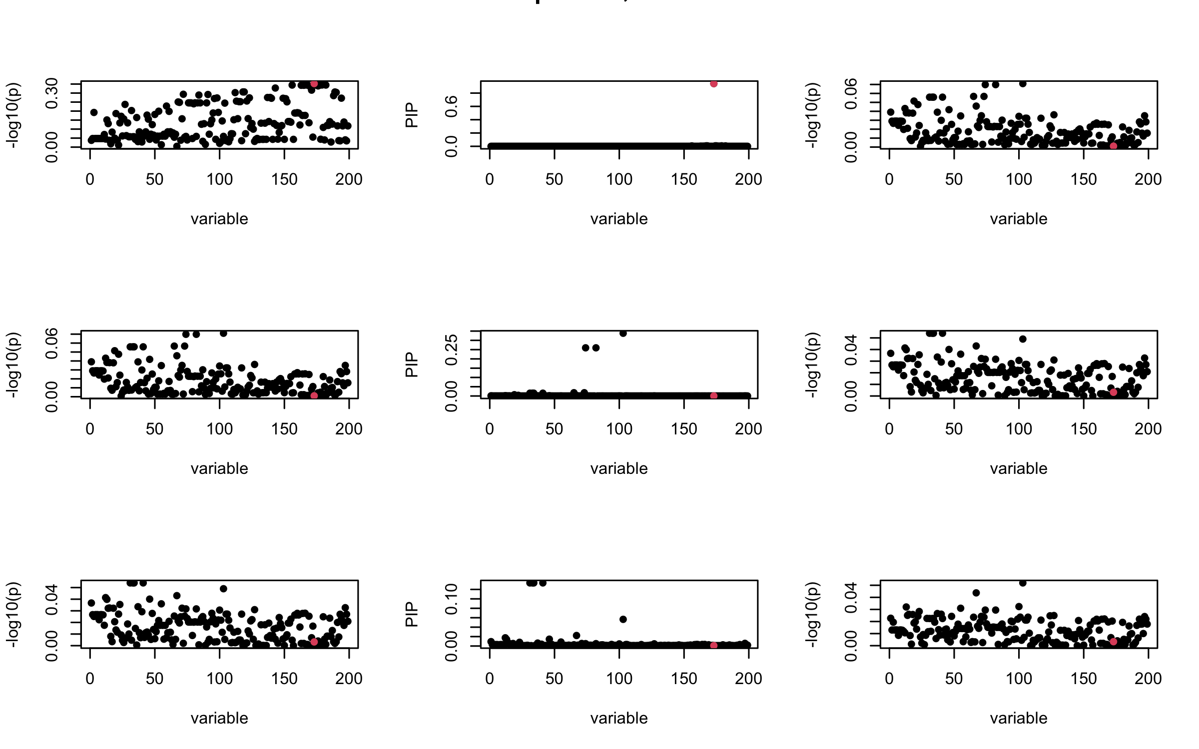
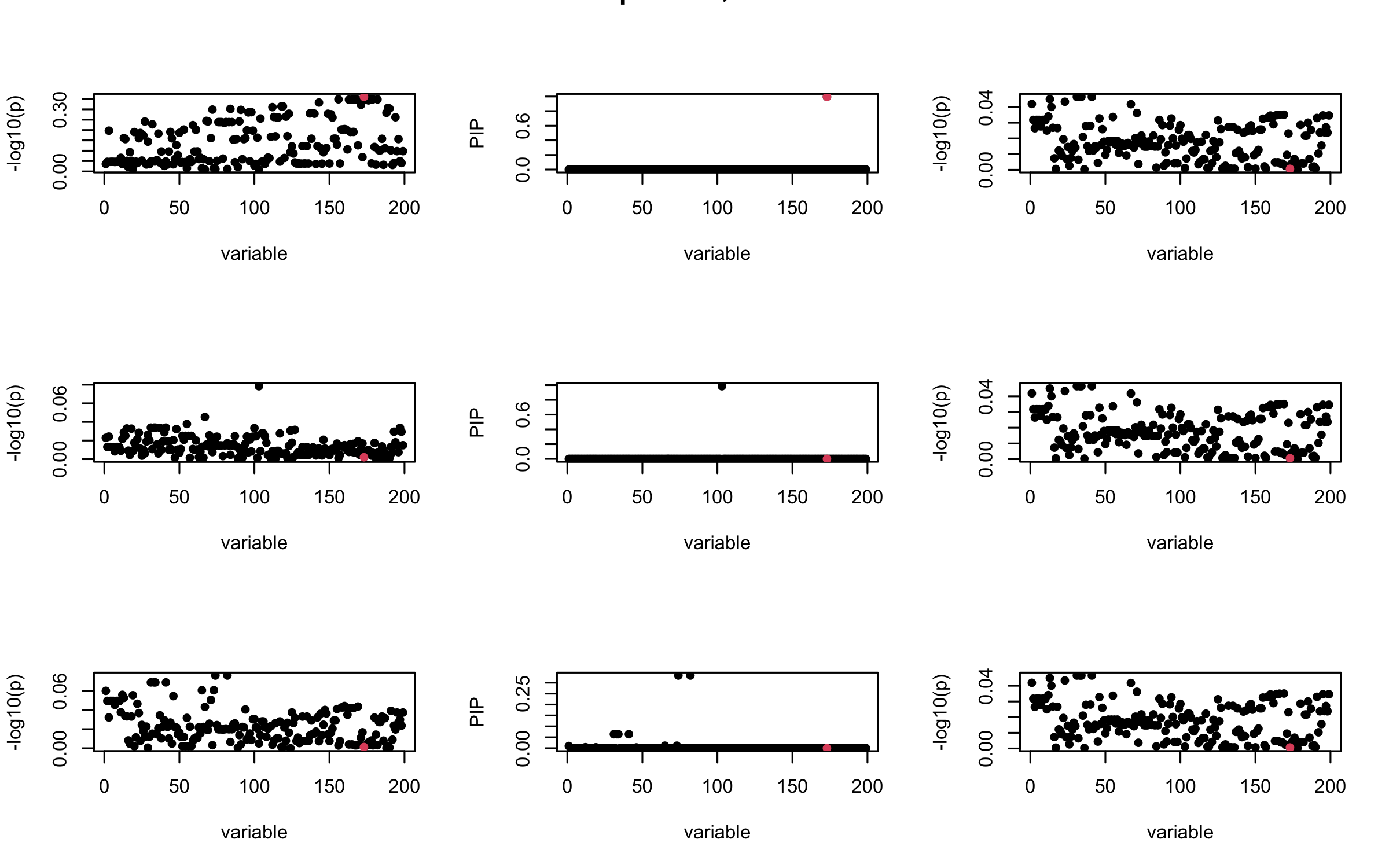
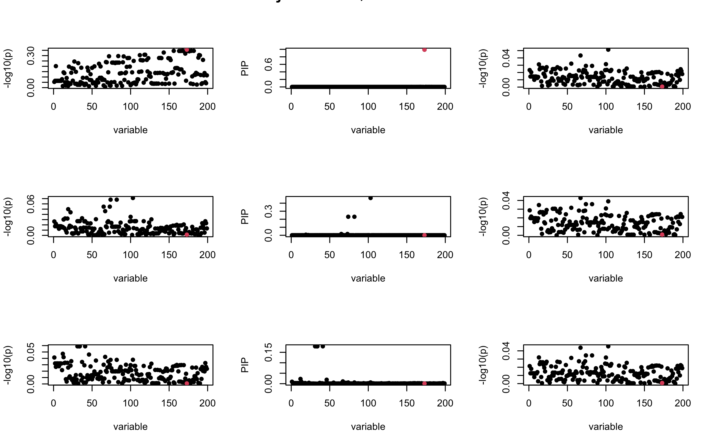
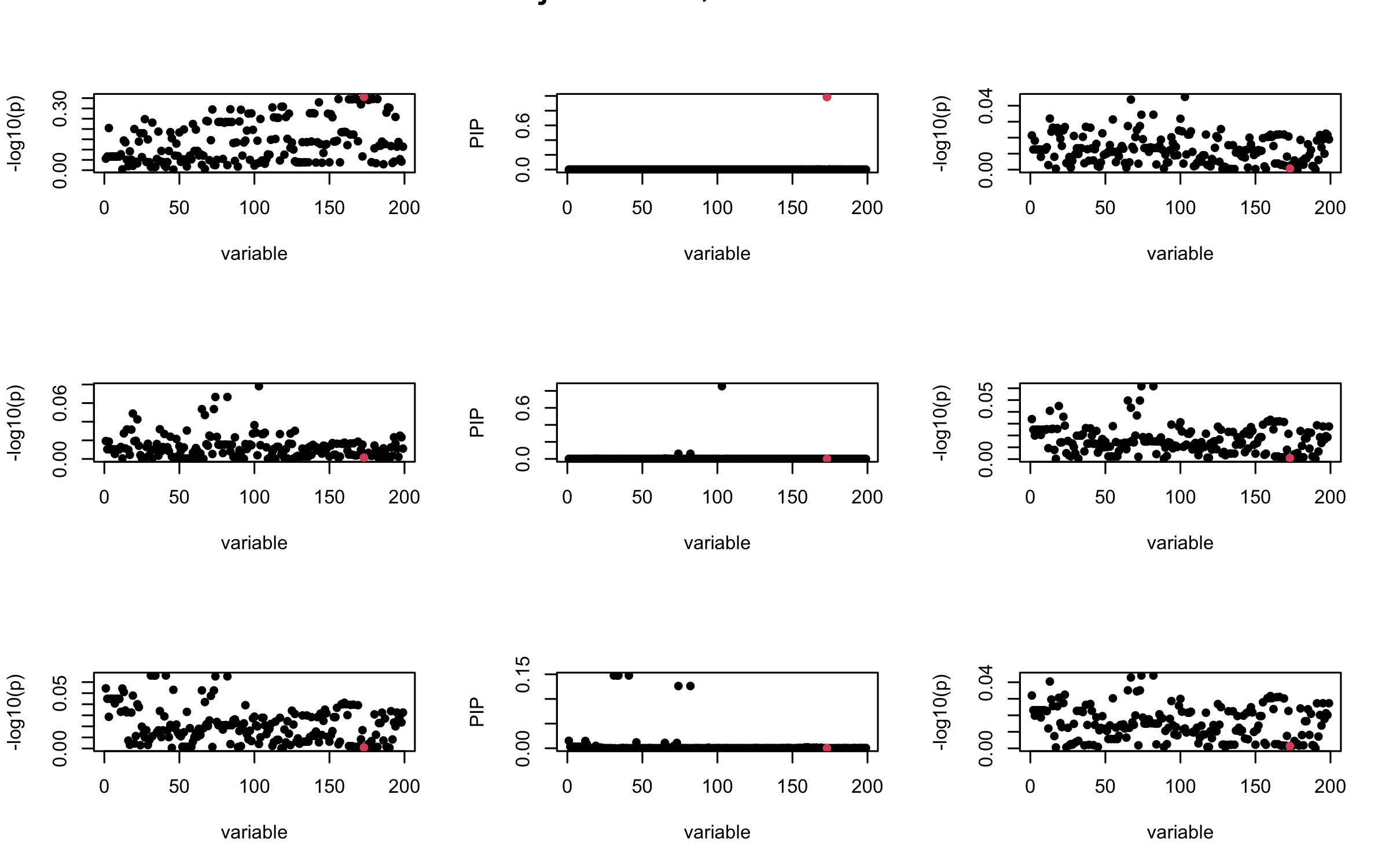
Here we want to investigate why using out-of-sample LD matrix can cause many false discovery by looking that the result after every training iteration. Recall that SuSiE_rss work by iteratively fitting Single Effect Model to the residuals: \[\overline{r} = X^{\top} y - X^{\top} X \overline{b} = v - R \overline{b} \] where \(\overline{b} = \sum_{\ell=1}^{L} \overline{b}_{\ell}\) is the sum of the posterior mean of all effects.
We expect that after detecting all ``true’’ casual SNP, \(\overline{r}\) will be a vector of \(J\) equally small numbers so that the PIP of over-fitted \(\ell\) will be close to 0 (diffused). Hence the purity of over-fitted \(\ell\)-th CS is small and is not reported.
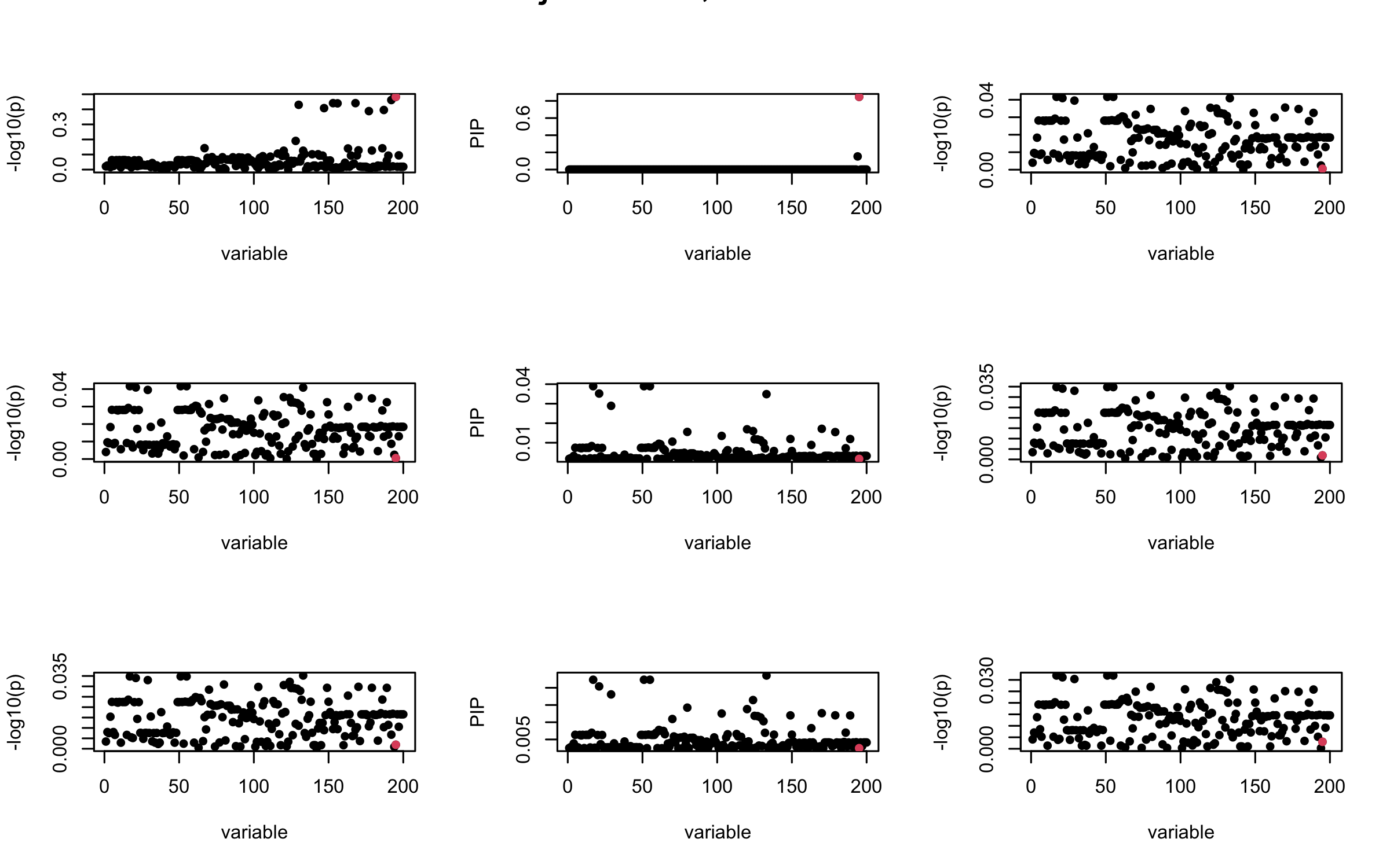
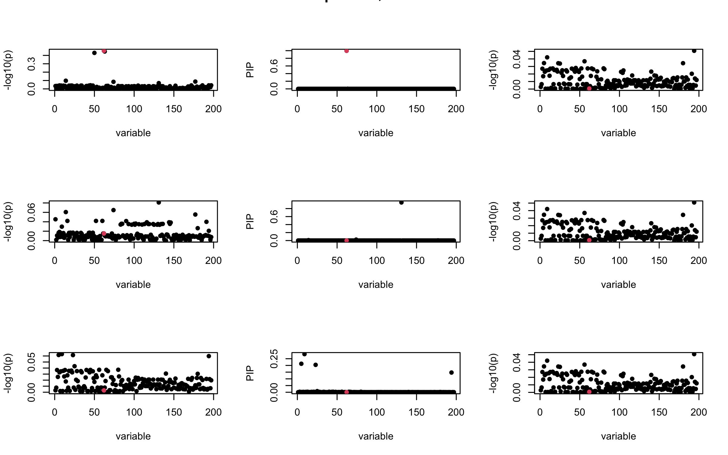
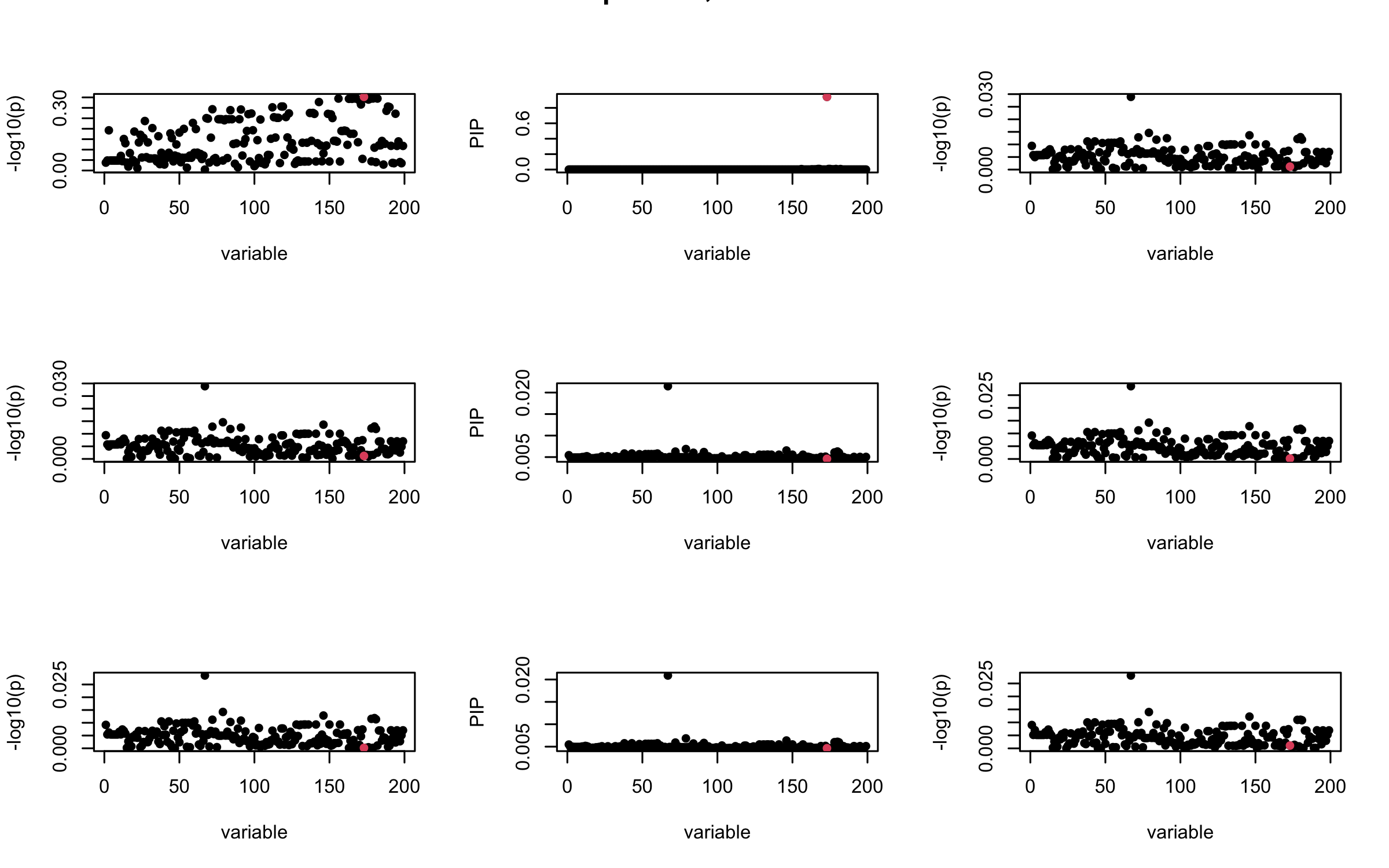
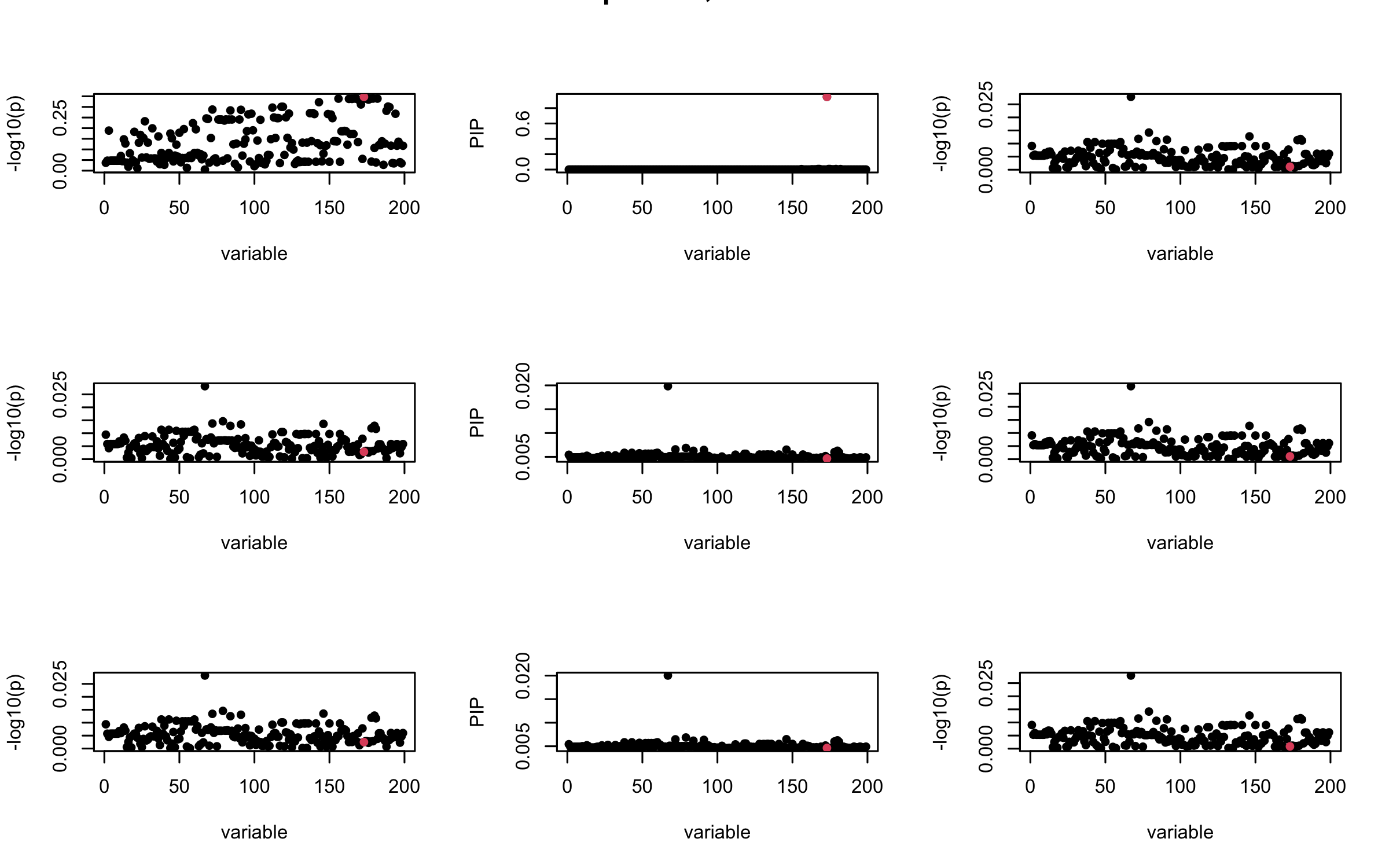
However, it can be seen that because of mis-specified \(R\), after controlling for all casual SNP, the residual \(\overline{r}\) of other SNPs can ``increase’’, leading to large PIP, thus creates false discovery.
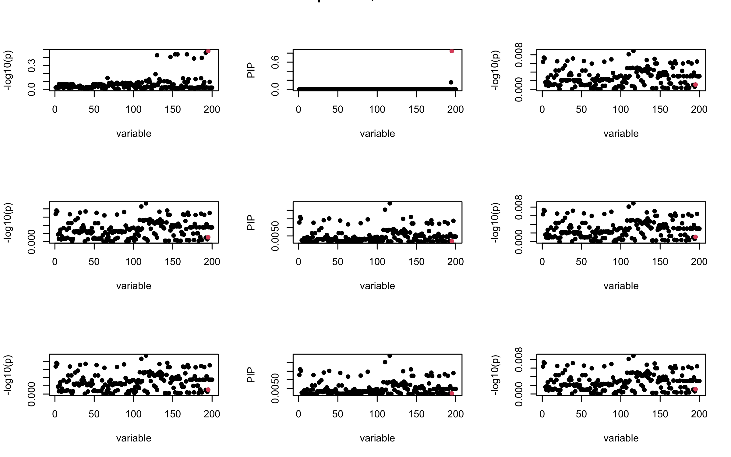
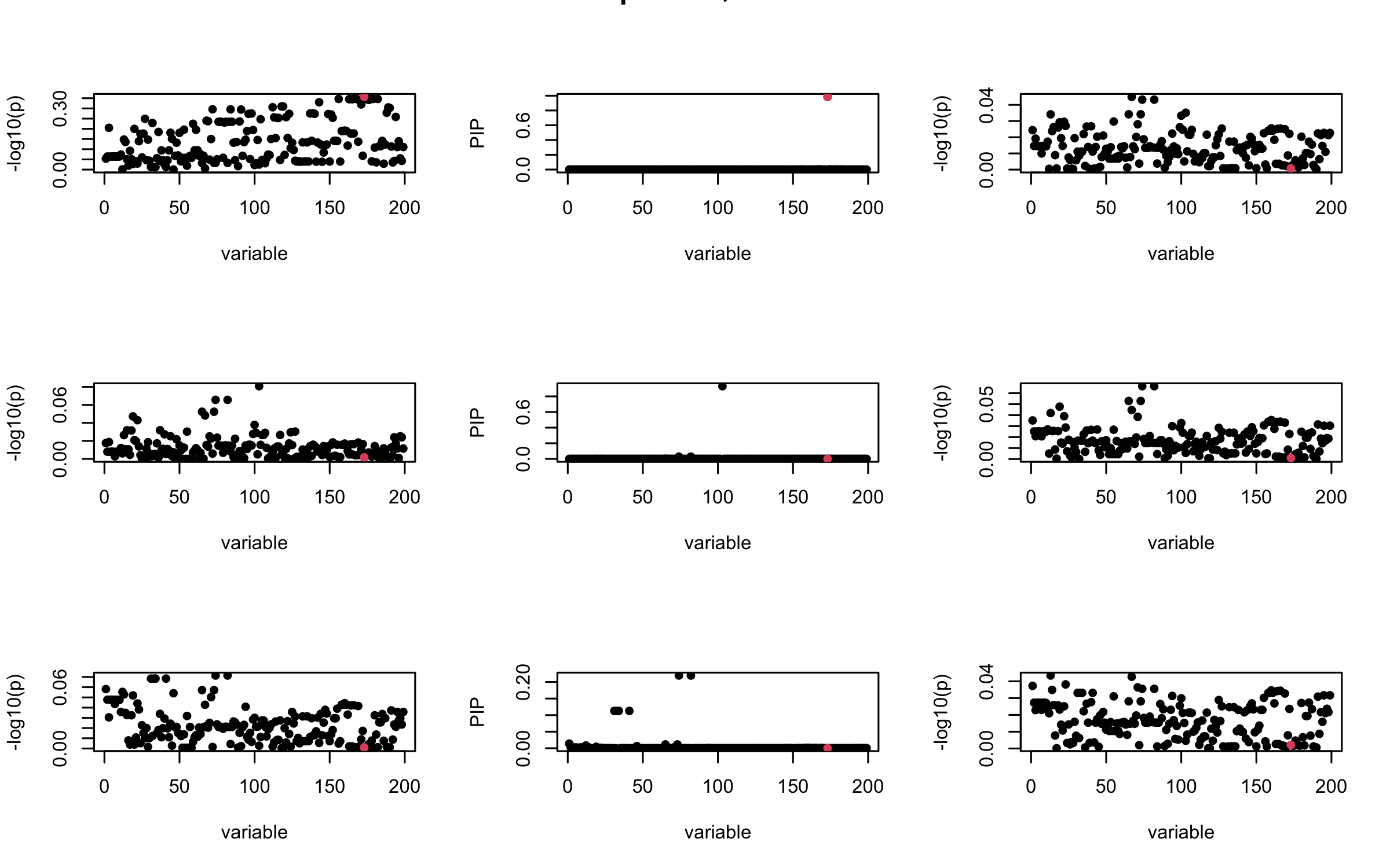
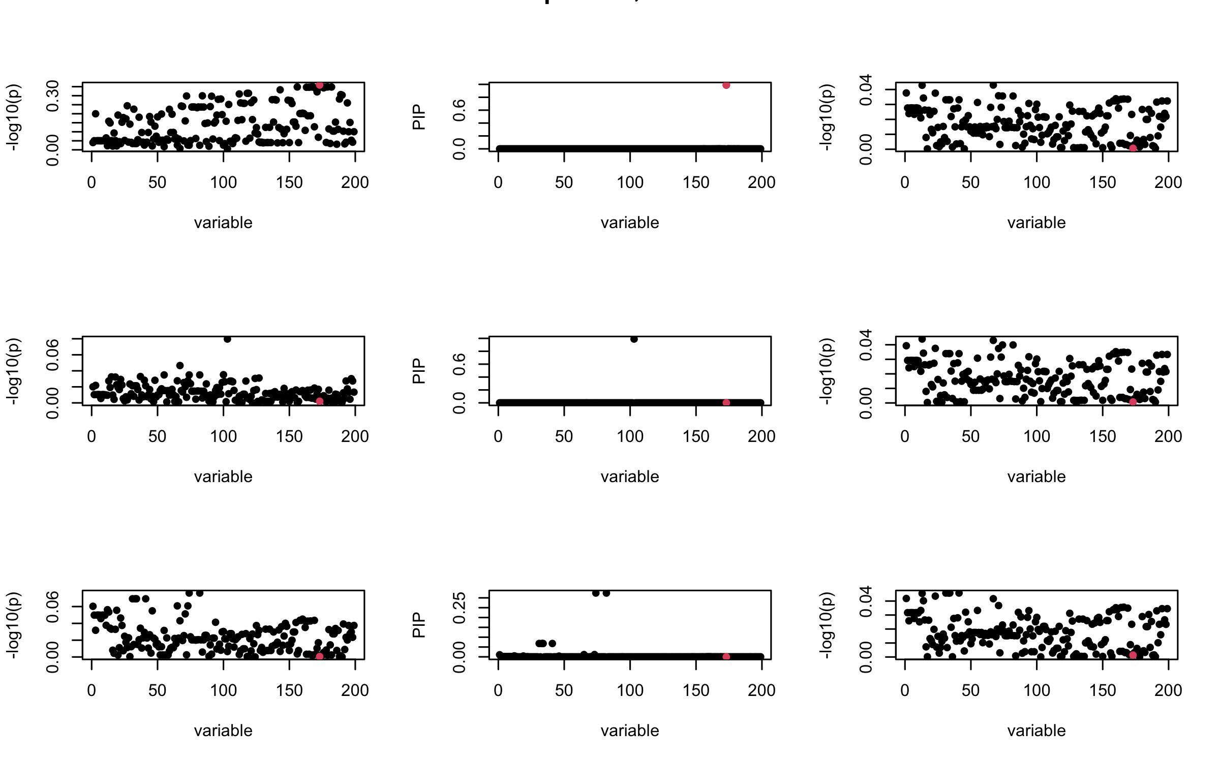
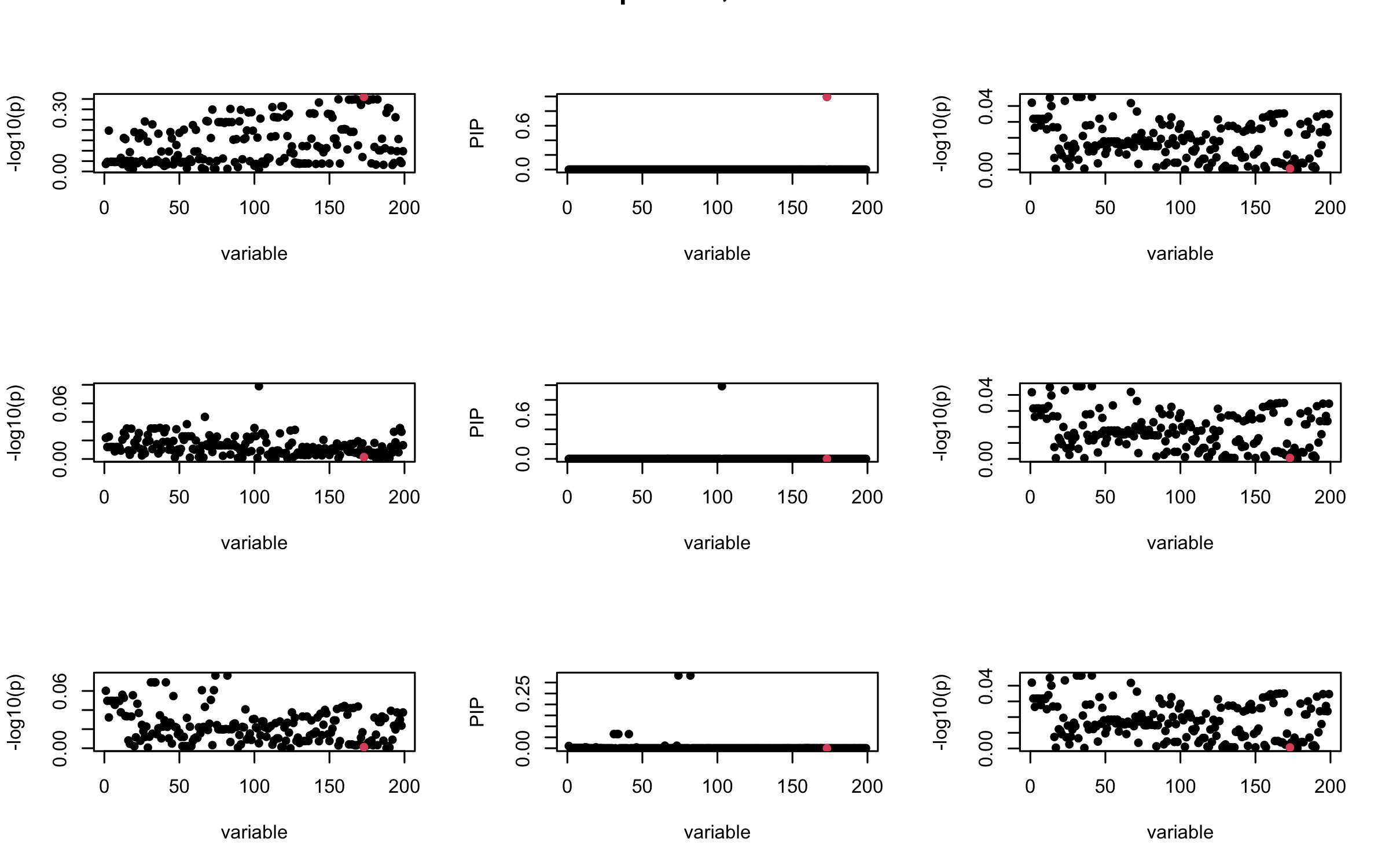
We will also see that our method (projected \(R\)) will experience this bad behavior much less.
In-sample Covariance matrix
Out-sample Covariance matrix
## 2. Out-sample covariance matrix
V_xx = R_hat
sigma2 = 1
sigma02 = 1
L = 3
max_iter = 10

b_bar = matrix(0, nrow = L, ncol = J)
b_bar2 = matrix(0, nrow = L, ncol = J)
alphas = matrix(0, nrow = L, ncol = J)
mus = matrix(0, nrow = L, ncol = J)
sigmas = matrix(0, nrow = L, ncol = J)


for (iter in (1:max_iter)){
  par(mfrow = c(3, 3))
  V_xy_bar = V_xy - V_xx %*% colSums(b_bar)  ## residual signal

  for (ell in 1:L){
    V_xy_bar_ell = V_xy_bar + V_xx %*% b_bar[ell, ]  ## add back ell-th signal

    susie_plot(V_xy_bar_ell, y = "z", b=beta)

    ret = SER(V_xx, V_xy_bar_ell, n, sigma2, sigma02)
    alphas[ell, ] = ret$alpha
    mus[ell, ] = ret$mus
    sigmas[ell, ] = ret$sigma12
    b_bar[ell, ] = alphas[ell, ] * mus[ell, ]
    b_bar2[ell, ] = alphas[ell, ] * (mus[ell, ]^2 + sigmas[ell, ])
    V_xy_bar = V_xy_bar_ell - V_xx %*% b_bar[ell, ]

    susie_plot(ret$alpha, y = "PIP", b=beta)
    susie_plot(V_xy_bar, y = "z", b=beta)

  }
  mtext(paste0("Out-sample R, Iteration ", iter), outer = TRUE, cex = 1.5)
}


Projected Covariance matrix
## 3. Projected R
ret = proj_Dykstra(R=R_hat, v=V_xy)
V_xx = ret$R
sigma2 = 1
sigma02 = 1
L = 3
max_iter = 10

b_bar = matrix(0, nrow = L, ncol = J)
b_bar2 = matrix(0, nrow = L, ncol = J)
alphas = matrix(0, nrow = L, ncol = J)
mus = matrix(0, nrow = L, ncol = J)
sigmas = matrix(0, nrow = L, ncol = J)


for (iter in (1:max_iter)){
  par(mfrow = c(3, 3))
  V_xy_bar = V_xy - V_xx %*% colSums(b_bar)  ## residual signal

  for (ell in 1:L){
    V_xy_bar_ell = V_xy_bar + V_xx %*% b_bar[ell, ]  ## add back ell-th signal

    susie_plot(V_xy_bar_ell, y = "z", b=beta)

    ret = SER(V_xx, V_xy_bar_ell, n, sigma2, sigma02)
    alphas[ell, ] = ret$alpha
    mus[ell, ] = ret$mus
    sigmas[ell, ] = ret$sigma12
    b_bar[ell, ] = alphas[ell, ] * mus[ell, ]
    b_bar2[ell, ] = alphas[ell, ] * (mus[ell, ]^2 + sigmas[ell, ])
    V_xy_bar = V_xy_bar_ell - V_xx %*% b_bar[ell, ]

    susie_plot(ret$alpha, y = "PIP", b=beta)
    susie_plot(V_xy_bar, y = "z", b=beta)

  }
  mtext(paste0("Projected R, Iteration ", iter), outer = TRUE, cex = 1.5)
}
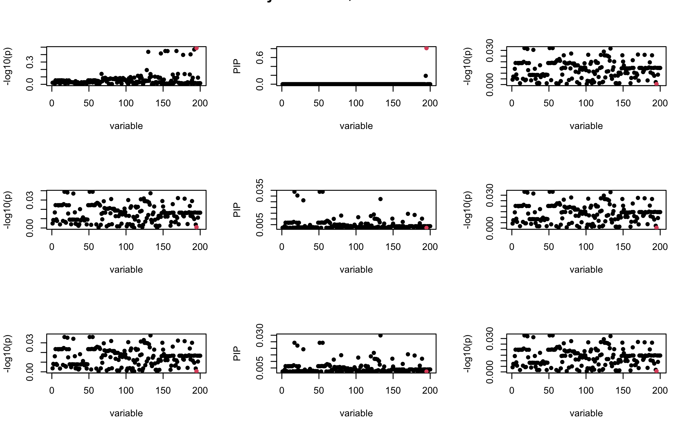


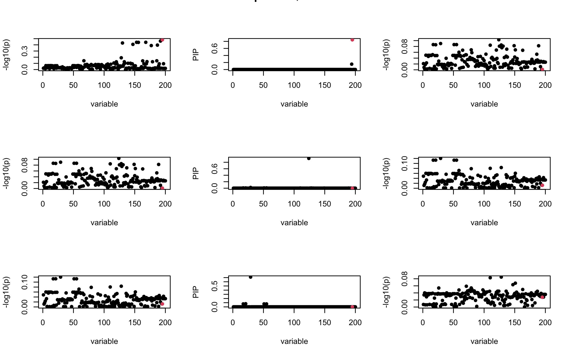
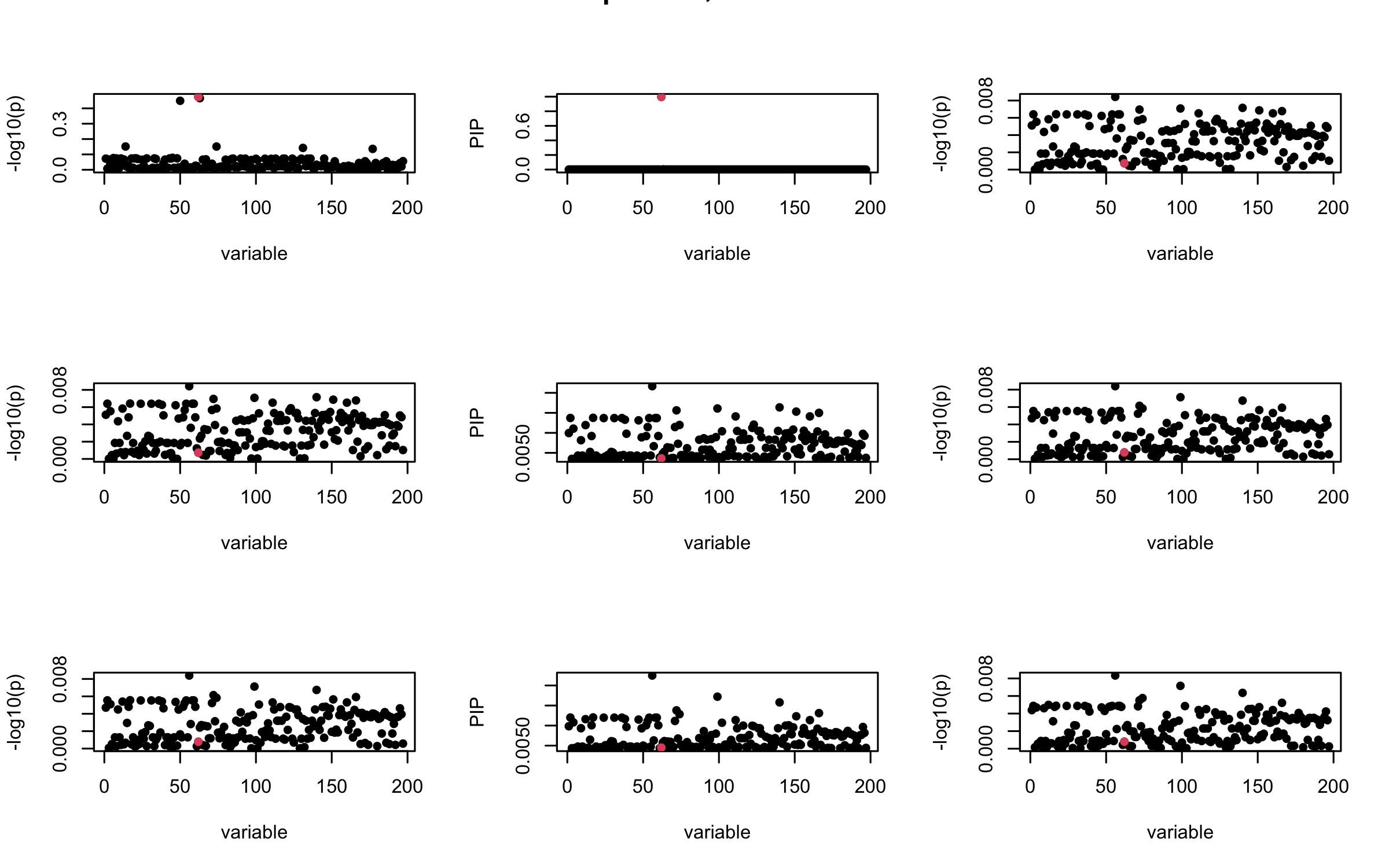
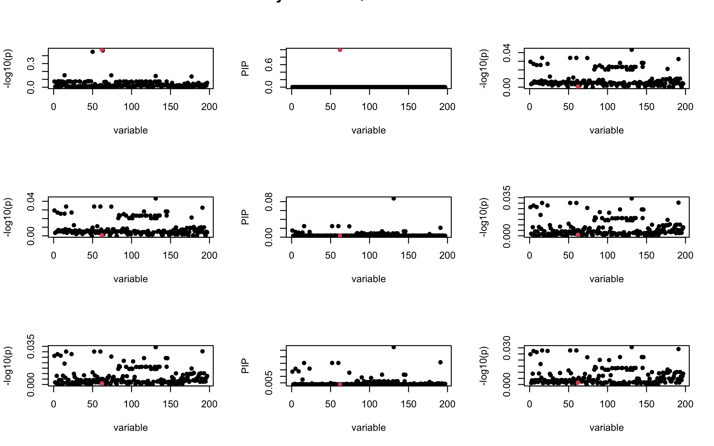
Let us look at some other seeds.
seed = 1
set.seed(seed)
print(paste("This is seed number", seed))
[1] "This is seed number 1"# Remove SNPs with MAF < 0.01
maf = apply(gtex, 2, function(x) sum(x)/2/length(x))
X0 = gtex[, maf > 0.01]
dim(X0)[1] 574 7154X = na.omit(X0)
dim(X)[1] 574 7154snp_total = ncol(X0)
n = nrow(X0)
J = 200
# Start from a random point on the genome
indx_start = sample(1: (snp_total - J), 1)
X = X0[, indx_start:(indx_start + J -1)]
# View(cor(X)[1:10, 1:10])
## sub-sample into two
out_sample = sample(1:n, 100)
X_out = X[out_sample, ]
X_in = X[setdiff(1:n, out_sample), ]
sum(is.na(X_out))[1] 0rm_p = c(which(diag(cov(X_in))==0), which(diag(cov(X_out))==0))
length(rm_p)[1] 0indx_p = setdiff(1:J, rm_p)
X_in = X_in[, indx_p]
X_out = X_out[, indx_p]
## Standardize both sample matrices
X_in <- scale(X_in)
X_out <- scale(X_out)
## out-sample LD matrix
R_hat = cor(X_out)
R = cor(X_in)
## generate data from in-sample X matrix
J = ncol(X_in)
beta <- rep(0, J)
n = nrow(X_in)
num_casual_SNP = 1
gamma = sample(c(1:J), size = num_casual_SNP, replace = FALSE)
b = rnorm(num_casual_SNP) * 3
beta = rep(0, J)
beta[gamma] = b
y = X_in %*% beta + rnorm(n)
y = scale(y)
V_xy = t(X_in) %*% y / (n-1)
## 1. In-sample covariance matrix
V_xx = R
sigma2 = 1
sigma02 = 1
L = 3
max_iter = 10
b_bar = matrix(0, nrow = L, ncol = J)
b_bar2 = matrix(0, nrow = L, ncol = J)
alphas = matrix(0, nrow = L, ncol = J)
mus = matrix(0, nrow = L, ncol = J)
sigmas = matrix(0, nrow = L, ncol = J)
for (iter in (1:max_iter)){
par(mfrow = c(3, 3))
V_xy_bar = V_xy - V_xx %*% colSums(b_bar) ## residual signal
for (ell in 1:L){
V_xy_bar_ell = V_xy_bar + V_xx %*% b_bar[ell, ] ## add back ell-th signal
susie_plot(V_xy_bar_ell, y = "z", b=beta)
ret = SER(V_xx, V_xy_bar_ell, n, sigma2, sigma02)
alphas[ell, ] = ret$alpha
mus[ell, ] = ret$mus
sigmas[ell, ] = ret$sigma12
b_bar[ell, ] = alphas[ell, ] * mus[ell, ]
b_bar2[ell, ] = alphas[ell, ] * (mus[ell, ]^2 + sigmas[ell, ])
V_xy_bar = V_xy_bar_ell - V_xx %*% b_bar[ell, ]
susie_plot(ret$alpha, y = "PIP", b=beta)
susie_plot(V_xy_bar, y = "z", b=beta)
}
mtext(paste0("In-sample R, Iteration ", iter), outer = TRUE, cex = 1.5)
}


## 2. Out-sample covariance matrix
V_xx = R_hat
sigma2 = 1
sigma02 = 1
L = 3
max_iter = 10

b_bar = matrix(0, nrow = L, ncol = J)
b_bar2 = matrix(0, nrow = L, ncol = J)
alphas = matrix(0, nrow = L, ncol = J)
mus = matrix(0, nrow = L, ncol = J)
sigmas = matrix(0, nrow = L, ncol = J)


for (iter in (1:max_iter)){
  par(mfrow = c(3, 3))
  V_xy_bar = V_xy - V_xx %*% colSums(b_bar)  ## residual signal

  for (ell in 1:L){
    V_xy_bar_ell = V_xy_bar + V_xx %*% b_bar[ell, ]  ## add back ell-th signal

    susie_plot(V_xy_bar_ell, y = "z", b=beta)

    ret = SER(V_xx, V_xy_bar_ell, n, sigma2, sigma02)
    alphas[ell, ] = ret$alpha
    mus[ell, ] = ret$mus
    sigmas[ell, ] = ret$sigma12
    b_bar[ell, ] = alphas[ell, ] * mus[ell, ]
    b_bar2[ell, ] = alphas[ell, ] * (mus[ell, ]^2 + sigmas[ell, ])
    V_xy_bar = V_xy_bar_ell - V_xx %*% b_bar[ell, ]

    susie_plot(ret$alpha, y = "PIP", b=beta)
    susie_plot(V_xy_bar, y = "z", b=beta)

  }
  mtext(paste0("Out-sample R, Iteration ", iter), outer = TRUE, cex = 1.5)
}


## 3. Projected R
ret = proj_Dykstra(R=R_hat, v=V_xy)
V_xx = ret$R
sigma2 = 1
sigma02 = 1
L = 3
max_iter = 10

b_bar = matrix(0, nrow = L, ncol = J)
b_bar2 = matrix(0, nrow = L, ncol = J)
alphas = matrix(0, nrow = L, ncol = J)
mus = matrix(0, nrow = L, ncol = J)
sigmas = matrix(0, nrow = L, ncol = J)


for (iter in (1:max_iter)){
  par(mfrow = c(3, 3))
  V_xy_bar = V_xy - V_xx %*% colSums(b_bar)  ## residual signal

  for (ell in 1:L){
    V_xy_bar_ell = V_xy_bar + V_xx %*% b_bar[ell, ]  ## add back ell-th signal

    susie_plot(V_xy_bar_ell, y = "z", b=beta)

    ret = SER(V_xx, V_xy_bar_ell, n, sigma2, sigma02)
    alphas[ell, ] = ret$alpha
    mus[ell, ] = ret$mus
    sigmas[ell, ] = ret$sigma12
    b_bar[ell, ] = alphas[ell, ] * mus[ell, ]
    b_bar2[ell, ] = alphas[ell, ] * (mus[ell, ]^2 + sigmas[ell, ])
    V_xy_bar = V_xy_bar_ell - V_xx %*% b_bar[ell, ]

    susie_plot(ret$alpha, y = "PIP", b=beta)
    susie_plot(V_xy_bar, y = "z", b=beta)

  }
  mtext(paste0("Projected R, Iteration ", iter), outer = TRUE, cex = 1.5)
}


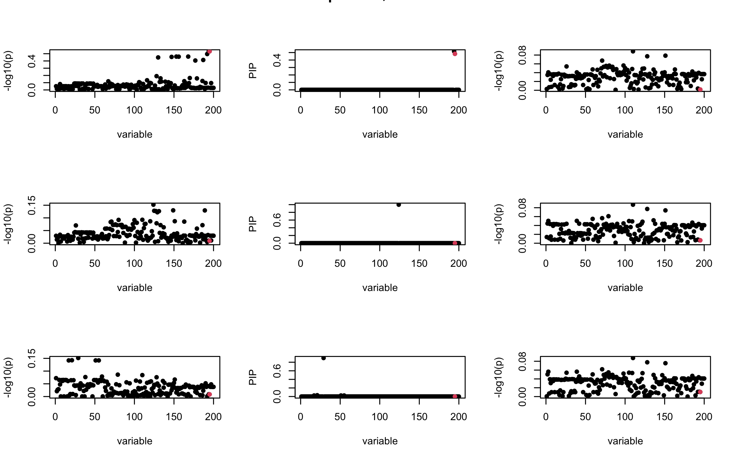
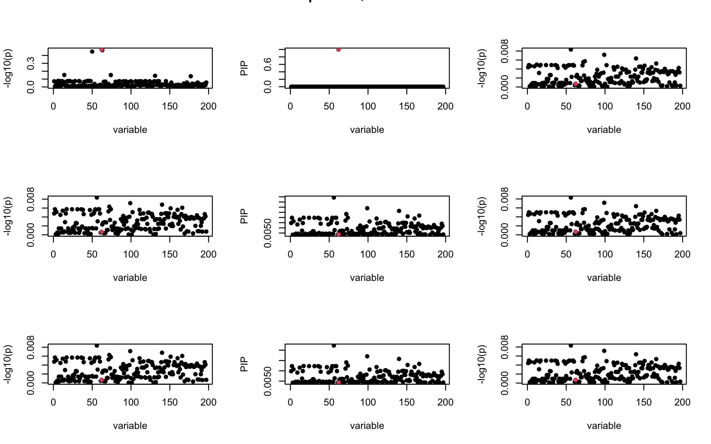
seed = 2
set.seed(seed)
print(paste("This is seed number", seed))
[1] "This is seed number 2"# Remove SNPs with MAF < 0.01
maf = apply(gtex, 2, function(x) sum(x)/2/length(x))
X0 = gtex[, maf > 0.01]
dim(X0)[1] 574 7154X = na.omit(X0)
dim(X)[1] 574 7154snp_total = ncol(X0)
n = nrow(X0)
J = 200
# Start from a random point on the genome
indx_start = sample(1: (snp_total - J), 1)
X = X0[, indx_start:(indx_start + J -1)]
# View(cor(X)[1:10, 1:10])
## sub-sample into two
out_sample = sample(1:n, 100)
X_out = X[out_sample, ]
X_in = X[setdiff(1:n, out_sample), ]
sum(is.na(X_out))[1] 0rm_p = c(which(diag(cov(X_in))==0), which(diag(cov(X_out))==0))
length(rm_p)[1] 3indx_p = setdiff(1:J, rm_p)
X_in = X_in[, indx_p]
X_out = X_out[, indx_p]
## Standardize both sample matrices
X_in <- scale(X_in)
X_out <- scale(X_out)
## out-sample LD matrix
R_hat = cor(X_out)
R = cor(X_in)
## generate data from in-sample X matrix
J = ncol(X_in)
beta <- rep(0, J)
n = nrow(X_in)
num_casual_SNP = 1
gamma = sample(c(1:J), size = num_casual_SNP, replace = FALSE)
b = rnorm(num_casual_SNP) * 3
beta = rep(0, J)
beta[gamma] = b
y = X_in %*% beta + rnorm(n)
y = scale(y)
V_xy = t(X_in) %*% y / (n-1)
## 1. In-sample covariance matrix
V_xx = R
sigma2 = 1
sigma02 = 1
L = 3
max_iter = 10
b_bar = matrix(0, nrow = L, ncol = J)
b_bar2 = matrix(0, nrow = L, ncol = J)
alphas = matrix(0, nrow = L, ncol = J)
mus = matrix(0, nrow = L, ncol = J)
sigmas = matrix(0, nrow = L, ncol = J)
for (iter in (1:max_iter)){
par(mfrow = c(3, 3))
V_xy_bar = V_xy - V_xx %*% colSums(b_bar) ## residual signal
for (ell in 1:L){
V_xy_bar_ell = V_xy_bar + V_xx %*% b_bar[ell, ] ## add back ell-th signal
susie_plot(V_xy_bar_ell, y = "z", b=beta)
ret = SER(V_xx, V_xy_bar_ell, n, sigma2, sigma02)
alphas[ell, ] = ret$alpha
mus[ell, ] = ret$mus
sigmas[ell, ] = ret$sigma12
b_bar[ell, ] = alphas[ell, ] * mus[ell, ]
b_bar2[ell, ] = alphas[ell, ] * (mus[ell, ]^2 + sigmas[ell, ])
V_xy_bar = V_xy_bar_ell - V_xx %*% b_bar[ell, ]
susie_plot(ret$alpha, y = "PIP", b=beta)
susie_plot(V_xy_bar, y = "z", b=beta)
}
mtext(paste0("In-sample R, Iteration ", iter), outer = TRUE, cex = 1.5)
}


## 2. Out-sample covariance matrix
V_xx = R_hat
sigma2 = 1
sigma02 = 1
L = 3
max_iter = 10

b_bar = matrix(0, nrow = L, ncol = J)
b_bar2 = matrix(0, nrow = L, ncol = J)
alphas = matrix(0, nrow = L, ncol = J)
mus = matrix(0, nrow = L, ncol = J)
sigmas = matrix(0, nrow = L, ncol = J)


for (iter in (1:max_iter)){
  par(mfrow = c(3, 3))
  V_xy_bar = V_xy - V_xx %*% colSums(b_bar)  ## residual signal

  for (ell in 1:L){
    V_xy_bar_ell = V_xy_bar + V_xx %*% b_bar[ell, ]  ## add back ell-th signal

    susie_plot(V_xy_bar_ell, y = "z", b=beta)

    ret = SER(V_xx, V_xy_bar_ell, n, sigma2, sigma02)
    alphas[ell, ] = ret$alpha
    mus[ell, ] = ret$mus
    sigmas[ell, ] = ret$sigma12
    b_bar[ell, ] = alphas[ell, ] * mus[ell, ]
    b_bar2[ell, ] = alphas[ell, ] * (mus[ell, ]^2 + sigmas[ell, ])
    V_xy_bar = V_xy_bar_ell - V_xx %*% b_bar[ell, ]

    susie_plot(ret$alpha, y = "PIP", b=beta)
    susie_plot(V_xy_bar, y = "z", b=beta)

  }
  mtext(paste0("Out-sample R, Iteration ", iter), outer = TRUE, cex = 1.5)
}


## 3. Projected R
ret = proj_Dykstra(R=R_hat, v=V_xy)
V_xx = ret$R
sigma2 = 1
sigma02 = 1
L = 3
max_iter = 10

b_bar = matrix(0, nrow = L, ncol = J)
b_bar2 = matrix(0, nrow = L, ncol = J)
alphas = matrix(0, nrow = L, ncol = J)
mus = matrix(0, nrow = L, ncol = J)
sigmas = matrix(0, nrow = L, ncol = J)


for (iter in (1:max_iter)){
  par(mfrow = c(3, 3))
  V_xy_bar = V_xy - V_xx %*% colSums(b_bar)  ## residual signal

  for (ell in 1:L){
    V_xy_bar_ell = V_xy_bar + V_xx %*% b_bar[ell, ]  ## add back ell-th signal

    susie_plot(V_xy_bar_ell, y = "z", b=beta)

    ret = SER(V_xx, V_xy_bar_ell, n, sigma2, sigma02)
    alphas[ell, ] = ret$alpha
    mus[ell, ] = ret$mus
    sigmas[ell, ] = ret$sigma12
    b_bar[ell, ] = alphas[ell, ] * mus[ell, ]
    b_bar2[ell, ] = alphas[ell, ] * (mus[ell, ]^2 + sigmas[ell, ])
    V_xy_bar = V_xy_bar_ell - V_xx %*% b_bar[ell, ]

    susie_plot(ret$alpha, y = "PIP", b=beta)
    susie_plot(V_xy_bar, y = "z", b=beta)

  }
  mtext(paste0("Projected R, Iteration ", iter), outer = TRUE, cex = 1.5)
}


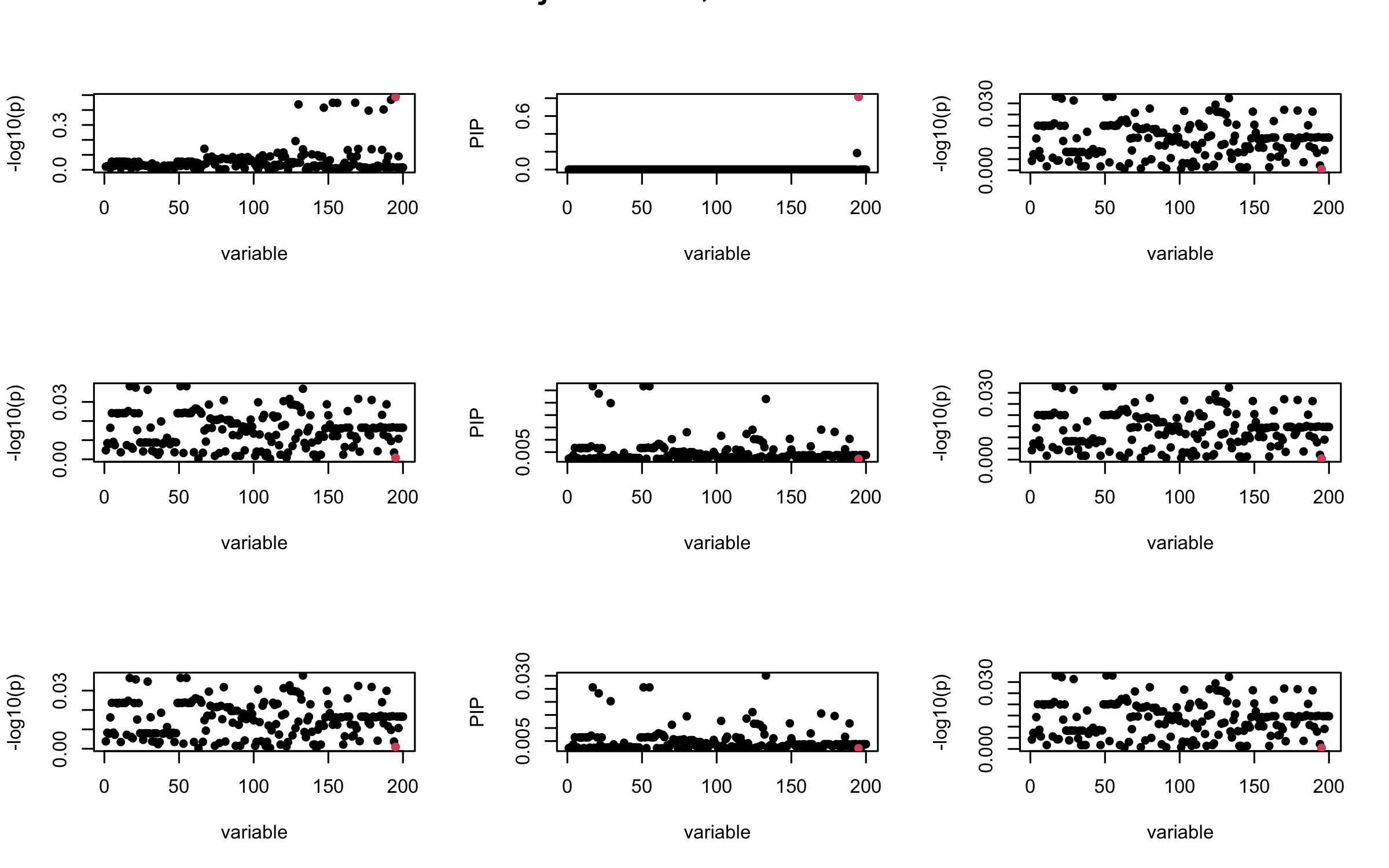
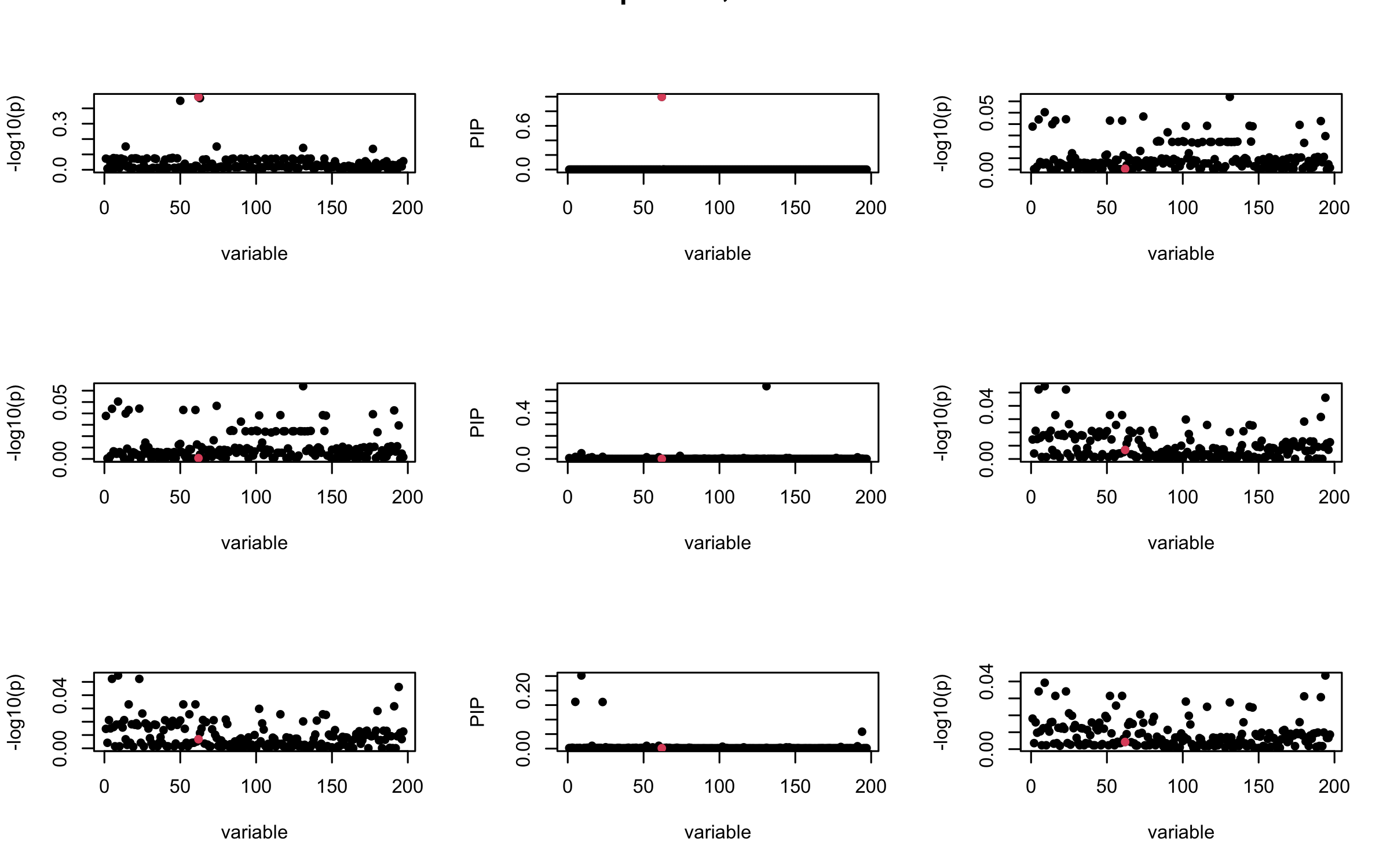
seed = 3
set.seed(seed)
print(paste("This is seed number", seed))
[1] "This is seed number 3"# Remove SNPs with MAF < 0.01
maf = apply(gtex, 2, function(x) sum(x)/2/length(x))
X0 = gtex[, maf > 0.01]
dim(X0)[1] 574 7154X = na.omit(X0)
dim(X)[1] 574 7154snp_total = ncol(X0)
n = nrow(X0)
J = 200
# Start from a random point on the genome
indx_start = sample(1: (snp_total - J), 1)
X = X0[, indx_start:(indx_start + J -1)]
# View(cor(X)[1:10, 1:10])
## sub-sample into two
out_sample = sample(1:n, 100)
X_out = X[out_sample, ]
X_in = X[setdiff(1:n, out_sample), ]
sum(is.na(X_out))[1] 0rm_p = c(which(diag(cov(X_in))==0), which(diag(cov(X_out))==0))
length(rm_p)[1] 1indx_p = setdiff(1:J, rm_p)
X_in = X_in[, indx_p]
X_out = X_out[, indx_p]
## Standardize both sample matrices
X_in <- scale(X_in)
X_out <- scale(X_out)
## out-sample LD matrix
R_hat = cor(X_out)
R = cor(X_in)
## generate data from in-sample X matrix
J = ncol(X_in)
beta <- rep(0, J)
n = nrow(X_in)
num_casual_SNP = 1
gamma = sample(c(1:J), size = num_casual_SNP, replace = FALSE)
b = rnorm(num_casual_SNP) * 3
beta = rep(0, J)
beta[gamma] = b
y = X_in %*% beta + rnorm(n)
y = scale(y)
V_xy = t(X_in) %*% y / (n-1)
## 1. In-sample covariance matrix
V_xx = R
sigma2 = 1
sigma02 = 1
L = 3
max_iter = 10
b_bar = matrix(0, nrow = L, ncol = J)
b_bar2 = matrix(0, nrow = L, ncol = J)
alphas = matrix(0, nrow = L, ncol = J)
mus = matrix(0, nrow = L, ncol = J)
sigmas = matrix(0, nrow = L, ncol = J)
for (iter in (1:max_iter)){
par(mfrow = c(3, 3))
V_xy_bar = V_xy - V_xx %*% colSums(b_bar) ## residual signal
for (ell in 1:L){
V_xy_bar_ell = V_xy_bar + V_xx %*% b_bar[ell, ] ## add back ell-th signal
susie_plot(V_xy_bar_ell, y = "z", b=beta)
ret = SER(V_xx, V_xy_bar_ell, n, sigma2, sigma02)
alphas[ell, ] = ret$alpha
mus[ell, ] = ret$mus
sigmas[ell, ] = ret$sigma12
b_bar[ell, ] = alphas[ell, ] * mus[ell, ]
b_bar2[ell, ] = alphas[ell, ] * (mus[ell, ]^2 + sigmas[ell, ])
V_xy_bar = V_xy_bar_ell - V_xx %*% b_bar[ell, ]
susie_plot(ret$alpha, y = "PIP", b=beta)
susie_plot(V_xy_bar, y = "z", b=beta)
}
mtext(paste0("In-sample R, Iteration ", iter), outer = TRUE, cex = 1.5)
}


## 2. Out-sample covariance matrix
V_xx = R_hat
sigma2 = 1
sigma02 = 1
L = 3
max_iter = 10

b_bar = matrix(0, nrow = L, ncol = J)
b_bar2 = matrix(0, nrow = L, ncol = J)
alphas = matrix(0, nrow = L, ncol = J)
mus = matrix(0, nrow = L, ncol = J)
sigmas = matrix(0, nrow = L, ncol = J)


for (iter in (1:max_iter)){
  par(mfrow = c(3, 3))
  V_xy_bar = V_xy - V_xx %*% colSums(b_bar)  ## residual signal

  for (ell in 1:L){
    V_xy_bar_ell = V_xy_bar + V_xx %*% b_bar[ell, ]  ## add back ell-th signal

    susie_plot(V_xy_bar_ell, y = "z", b=beta)

    ret = SER(V_xx, V_xy_bar_ell, n, sigma2, sigma02)
    alphas[ell, ] = ret$alpha
    mus[ell, ] = ret$mus
    sigmas[ell, ] = ret$sigma12
    b_bar[ell, ] = alphas[ell, ] * mus[ell, ]
    b_bar2[ell, ] = alphas[ell, ] * (mus[ell, ]^2 + sigmas[ell, ])
    V_xy_bar = V_xy_bar_ell - V_xx %*% b_bar[ell, ]

    susie_plot(ret$alpha, y = "PIP", b=beta)
    susie_plot(V_xy_bar, y = "z", b=beta)

  }
  mtext(paste0("Out-sample R, Iteration ", iter), outer = TRUE, cex = 1.5)
}


## 3. Projected R
ret = proj_Dykstra(R=R_hat, v=V_xy)
V_xx = ret$R
sigma2 = 1
sigma02 = 1
L = 3
max_iter = 10

b_bar = matrix(0, nrow = L, ncol = J)
b_bar2 = matrix(0, nrow = L, ncol = J)
alphas = matrix(0, nrow = L, ncol = J)
mus = matrix(0, nrow = L, ncol = J)
sigmas = matrix(0, nrow = L, ncol = J)


for (iter in (1:max_iter)){
  par(mfrow = c(3, 3))
  V_xy_bar = V_xy - V_xx %*% colSums(b_bar)  ## residual signal

  for (ell in 1:L){
    V_xy_bar_ell = V_xy_bar + V_xx %*% b_bar[ell, ]  ## add back ell-th signal

    susie_plot(V_xy_bar_ell, y = "z", b=beta)

    ret = SER(V_xx, V_xy_bar_ell, n, sigma2, sigma02)
    alphas[ell, ] = ret$alpha
    mus[ell, ] = ret$mus
    sigmas[ell, ] = ret$sigma12
    b_bar[ell, ] = alphas[ell, ] * mus[ell, ]
    b_bar2[ell, ] = alphas[ell, ] * (mus[ell, ]^2 + sigmas[ell, ])
    V_xy_bar = V_xy_bar_ell - V_xx %*% b_bar[ell, ]

    susie_plot(ret$alpha, y = "PIP", b=beta)
    susie_plot(V_xy_bar, y = "z", b=beta)

  }
  mtext(paste0("Projected R, Iteration ", iter), outer = TRUE, cex = 1.5)
}
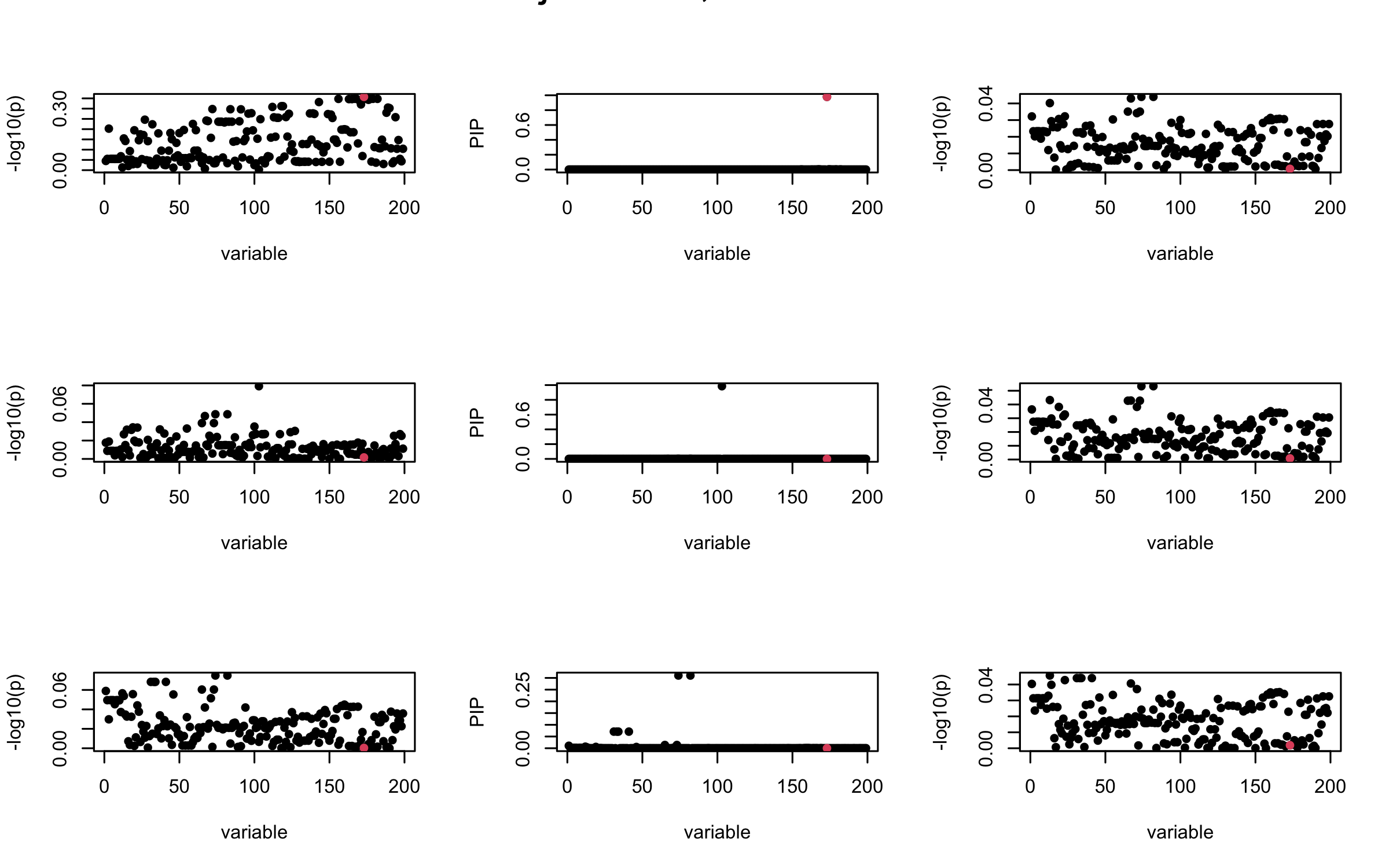


It remains a question whether we can make it as good as the in-sample LD matrix…
sessionInfo()R version 4.5.1 (2025-06-13)
Platform: aarch64-apple-darwin20
Running under: macOS Sequoia 15.6.1
Matrix products: default
BLAS: /Library/Frameworks/R.framework/Versions/4.5-arm64/Resources/lib/libRblas.0.dylib
LAPACK: /Library/Frameworks/R.framework/Versions/4.5-arm64/Resources/lib/libRlapack.dylib; LAPACK version 3.12.1
locale:
[1] en_US.UTF-8/en_US.UTF-8/en_US.UTF-8/C/en_US.UTF-8/en_US.UTF-8
time zone: America/Chicago
tzcode source: internal
attached base packages:
[1] stats graphics grDevices utils datasets methods base
other attached packages:
[1] RSpectra_0.16-2 Matrix_1.7-3 susieR_0.14.2 workflowr_1.7.1
loaded via a namespace (and not attached):
[1] sass_0.4.10 generics_0.1.4 stringi_1.8.7 lattice_0.22-7
[5] digest_0.6.37 magrittr_2.0.3 evaluate_1.0.4 grid_4.5.1
[9] RColorBrewer_1.1-3 fastmap_1.2.0 plyr_1.8.9 rprojroot_2.1.0
[13] jsonlite_2.0.0 processx_3.8.6 whisker_0.4.1 reshape_0.8.10
[17] ps_1.9.1 mixsqp_0.3-54 promises_1.3.3 httr_1.4.7
[21] scales_1.4.0 jquerylib_0.1.4 cli_3.6.5 rlang_1.1.6
[25] crayon_1.5.3 cachem_1.1.0 yaml_2.3.10 tools_4.5.1
[29] dplyr_1.1.4 ggplot2_3.5.2 httpuv_1.6.16 vctrs_0.6.5
[33] R6_2.6.1 matrixStats_1.5.0 lifecycle_1.0.4 git2r_0.36.2
[37] stringr_1.5.1 fs_1.6.6 irlba_2.3.5.1 pkgconfig_2.0.3
[41] callr_3.7.6 pillar_1.11.0 bslib_0.9.0 later_1.4.2
[45] gtable_0.3.6 glue_1.8.0 Rcpp_1.1.0 xfun_0.52
[49] tibble_3.3.0 tidyselect_1.2.1 rstudioapi_0.17.1 knitr_1.50
[53] farver_2.1.2 htmltools_0.5.8.1 rmarkdown_2.29 compiler_4.5.1
[57] getPass_0.2-4