Investigate Rank and Inverse-Wishart fit of N3finemapping data
Last updated: 2025-12-02
Checks: 7 0
Knit directory: Improved_LD_SuSiE/
This reproducible R Markdown analysis was created with workflowr (version 1.7.2). The Checks tab describes the reproducibility checks that were applied when the results were created. The Past versions tab lists the development history.
Great! Since the R Markdown file has been committed to the Git repository, you know the exact version of the code that produced these results.
Great job! The global environment was empty. Objects defined in the global environment can affect the analysis in your R Markdown file in unknown ways. For reproduciblity it’s best to always run the code in an empty environment.
The command set.seed(20250821) was run prior to running
the code in the R Markdown file. Setting a seed ensures that any results
that rely on randomness, e.g. subsampling or permutations, are
reproducible.
Great job! Recording the operating system, R version, and package versions is critical for reproducibility.
Nice! There were no cached chunks for this analysis, so you can be confident that you successfully produced the results during this run.
Great job! Using relative paths to the files within your workflowr project makes it easier to run your code on other machines.
Great! You are using Git for version control. Tracking code development and connecting the code version to the results is critical for reproducibility.
The results in this page were generated with repository version feb8208. See the Past versions tab to see a history of the changes made to the R Markdown and HTML files.
Note that you need to be careful to ensure that all relevant files for
the analysis have been committed to Git prior to generating the results
(you can use wflow_publish or
wflow_git_commit). workflowr only checks the R Markdown
file, but you know if there are other scripts or data files that it
depends on. Below is the status of the Git repository when the results
were generated:
Ignored files:
    Ignored:    .DS_Store

Unstaged changes:
    Modified:   code_push.R
Note that any generated files, e.g. HTML, png, CSS, etc., are not included in this status report because it is ok for generated content to have uncommitted changes.
These are the previous versions of the repository in which changes were
made to the R Markdown
(analysis/nu-matrix-F-distribution.Rmd) and HTML
(docs/nu-matrix-F-distribution.html) files. If you’ve
configured a remote Git repository (see ?wflow_git_remote),
click on the hyperlinks in the table below to view the files as they
were in that past version.
| File | Version | Author | Date | Message |
|---|---|---|---|---|
| html | d3b0e4f | dodat97 | 2025-12-02 | Build site. |
| Rmd | 153ece7 | dodat97 | 2025-12-02 | wflow_publish(c("analysis/nu-matrix-F-distribution.Rmd", "analysis/genotype-matrix-rank-investigation.Rmd")) |
| html | fc2f9c8 | dodat | 2025-12-02 | Build site. |
| Rmd | 9d9f457 | dodat | 2025-12-02 | wflow_publish(c("analysis/nu-matrix-F-distribution.Rmd")) |
library(susieR)
library(Matrix)

data(N3finemapping)
attach(N3finemapping)
X0 = N3finemapping$X
## getting covariance matrix from the whole sample
## and examine the eigendecomposition to estimate numerical rank
R = cov(X0)
eig <- eigen(R)
plot(eig$values,
     main = "Eigenvalues of covariance matrix calculated using all samples",
     ylab = "Value",
     xlab = "Eigenvalue index")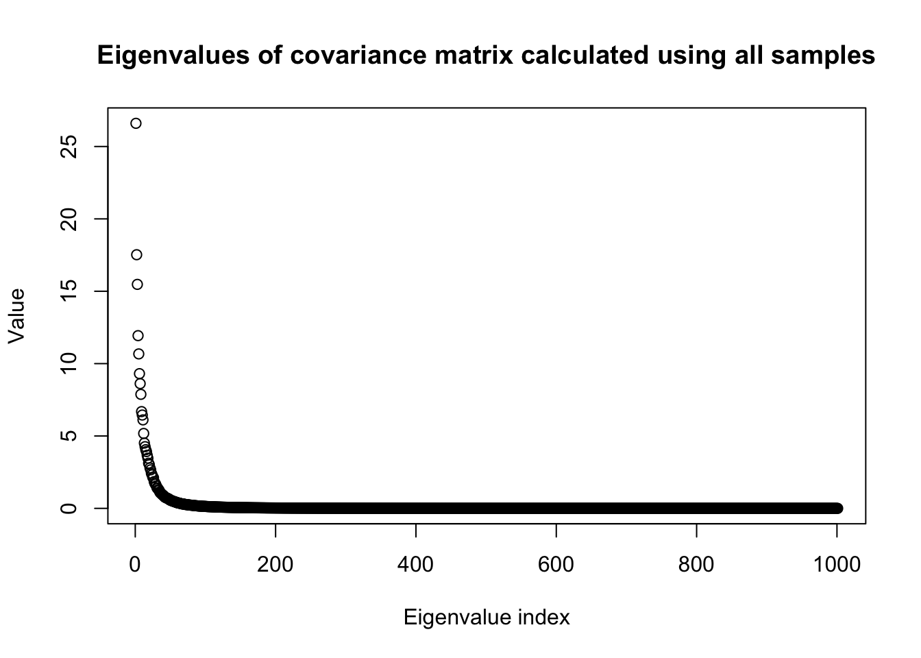
| Version | Author | Date |
|---|---|---|
| fc2f9c8 | dodat | 2025-12-02 |
n0 = dim(X0)[1]
p0 = dim(X0)[2]
percent_explained = .95
eig_cumsum = cumsum(eig$values)
r_p = sum(eig_cumsum < percent_explained * eig_cumsum[p0]) ## percentage variance explained
sprintf("%d first principle components explain %.1f percent of variance", r_p, percent_explained*100)
[1] "82 first principle components explain 95.0 percent of variance"snp_total = p0
sprintf("Total number of SNPs is %d", p0)[1] "Total number of SNPs is 1001"sprintf("Sample size %d", n0)[1] "Sample size 574"Now we proceed to split the data into half and look at the heatmap of the covariance matrices of two sub-samples.
#### randomly split the data into half
#### randomly select p consecutive SNPs where p < n so IW is proper
seed = 3
p = 50
# Start from a random point on the genome
indx_start = sample(1: (snp_total - p), 1)
X = X0[, indx_start:(indx_start + p -1)]
# View(cor(X)[1:10, 1:10])
## sub-sample into two
out_sample_size = n0 / 2
out_sample = sample(1:n0, out_sample_size)
X_out = X[out_sample, ]
X_in = X[setdiff(1:n0, out_sample), ]

rm_p = c(which(diag(cov(X_in))==0), which(diag(cov(X_out))==0))
indx_p = setdiff(1:p, rm_p)
X_in = X_in[, indx_p]
X_out = X_out[, indx_p]
## out-sample LD matrix
p = length(indx_p)
Rp = cov(X_out)
R0 = cov(X_in)
library(ggplot2)
library(reshape2)
df1 <- melt(R0)
df2 <- melt(Rp)
N_in = nrow(X_in)
N_out = nrow(X_out)
p1 <- ggplot(df1, aes(Var1, Var2, fill = value)) +
  geom_tile() +
  scale_fill_gradient2(low="blue", mid="white", high="red") +
  coord_fixed() +
  ggtitle(sprintf("In-sample Cov, %d samples", nrow(X_in)))
p2 <- ggplot(df2, aes(Var1, Var2, fill = value)) +
  geom_tile() +
  scale_fill_gradient2(low="blue", mid="white", high="red") +
  coord_fixed() +
  ggtitle(sprintf("Out-of-sample Cov, %d samples", nrow(X_out)))
library(gridExtra)
grid.arrange(p1, p2, ncol = 2)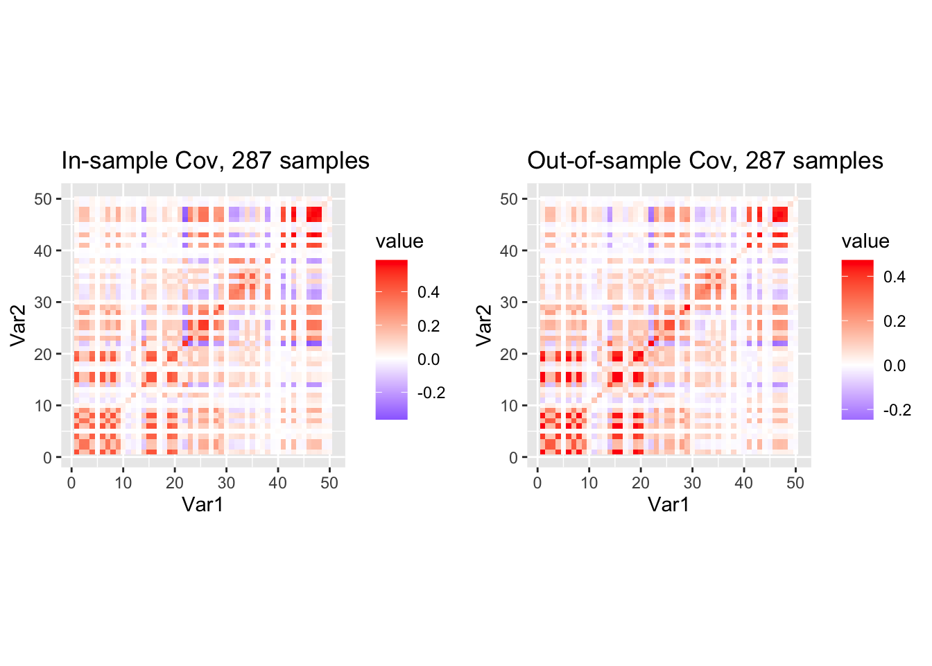
| Version | Author | Date |
|---|---|---|
| fc2f9c8 | dodat | 2025-12-02 |
Now let us consider modeling the in-sample covariance matrix \(R_0\) using the matrix F-distribution. We will consider two models: (1) one has mean being equal to the out-of-sample covariance matrix \(R'\) and (2) one has mean being equal to the “population” out-of-sample covariance matrix \(\Psi'\) (where we will learn \(\Psi'\) using Probabilistic PCA).
Firstly, when modeling \(R | \Psi \sim \mathcal{W}(\Psi / N, N)\) and \(\Psi | R' \sim \mathcal{IW}(\nu R', \nu + p + 1)\), we will have
\[R | R' \sim \mathrm{F}\left(\dfrac{\nu}{N} R', N, \nu + 2\right) \] This distribution has two degree-of-freedoms \(N\) and \(\nu+2\). It has mean \(R'\) and density:
\[p(R) = \dfrac{\Gamma_{\! p} \left(\tfrac{N + \nu + p + 1}{2}\right)}{\Gamma_{\! p} \left(\tfrac{N}{2}\right) \Gamma_{\! p} \left(\tfrac{\nu + p + 1}{2}\right)} \left| \dfrac{\nu R'}{N} \right|^{- N / 2} |R|^{(N - p - 1) / 2} \left|I + \dfrac{N}{\nu} R (R')^{-1}\right|^{-(N + \nu + p + 1) / 2},\] equivalently, \[p(R) = \dfrac{\Gamma_{\! p} \left(\tfrac{N + \nu + p + 1}{2}\right)}{\Gamma_{\! p} \left(\tfrac{N}{2}\right) \Gamma_{\! p} \left(\tfrac{\nu + p + 1}{2}\right)} \left| \dfrac{\nu R'}{N} \right|^{(\nu + p + 1) / 2} |R|^{(N - p - 1) / 2} \left|R + \dfrac{\nu}{N} R'\right|^{-(N + \nu + p + 1) / 2}.\]
## Matrix F-distribution likelihood
#### log F(R0 | nu * Rp / N, N, nu + 2)
log_multigamma_vec <- function(a, p) {
  # vectorized multivariate gamma
  j <- 1:p
  # sum over j, but broadcasting a over j
  (p*(p-1)/4)*log(pi) +
    rowSums(matrix(lgamma(a), nrow=length(a), ncol=p, byrow=FALSE) +
              matrix((1 - j)/2, nrow=length(a), ncol=p, byrow=TRUE))
}

log_F <- function(R0, Rp, N, nu_vec) {
  p <- nrow(R0)
  jitter = 1e-8
  R0 = R0 + jitter * diag(p)
  Rp = Rp + jitter * diag(p)
  # Precompute expensive shared quantities
  logdet_nu_Rp_over_N <- (determinant(Rp, logarithm = TRUE)$modulus
                          + p * log(nu_vec)
                          - p * log(N))
  logdetR0   <- determinant(R0, logarithm = TRUE)$modulus

  # lambda_vec <- eigen(solve(Rp, R0))$values
  # lambda_over_nu = tcrossprod(lambda_vec, N / nu_vec)
  # logdet_I_plus_RR <- colSums(log(1 + lambda_over_nu))
  # llhs = (log_multigamma_vec((N + nu_vec + p + 1) / 2, p)
  #         - log_multigamma_vec(N / 2, p)
  #         - log_multigamma_vec((nu_vec + p + 1) / 2, p)
  #         - .5 * N * logdet_nu_Rp_over_N
  #         + .5 * (N - p - 1) * logdetR0
  #         - .5 * (N + nu_vec + p + 1) * logdet_I_plus_RR)

  logdet_Rplus_Rp = rep(0, length(nu_vec))
  for (idx in 1:length(nu_vec)){
    nu = nu_vec[idx]
    logdet_Rplus_Rp[idx] <- determinant(R0 + nu * Rp / N, logarithm = TRUE)$modulus
  }

  llhs = (log_multigamma_vec((N + nu_vec + p + 1) / 2, p)
          - log_multigamma_vec(N / 2, p)
          - log_multigamma_vec((nu_vec + p + 1) / 2, p)
          + .5 * (nu_vec + p + 1) * logdet_nu_Rp_over_N
          + .5 * (N - p - 1) * logdetR0
          - .5 * (N + nu_vec + p + 1) * logdet_Rplus_Rp)

  as.numeric(llhs)
}

log_iw <- function(R0, Rp, nu_vec) {
  p <- nrow(R0)
  jitter = 1e-12
  R0 = R0 + jitter * diag(p)
  Rp = Rp + jitter * diag(p)
  # Precompute expensive shared quantities
  logdet_nu_Rp <- determinant(Rp, logarithm = TRUE)$modulus + p * log(nu_vec)
  logdetR0   <- determinant(R0,   logarithm = TRUE)$modulus
  tr_term   <- nu_vec * sum(t(Rp) * solve(R0))
  llhs = (.5 * (nu_vec + p + 1) * logdet_nu_Rp
          - .5 * (nu_vec + p + 1) * p * log(2)
          - log_multigamma_vec((nu_vec + p + 1) / 2, p)
          - .5 * (nu_vec + 2 * (p + 1)) * logdetR0
          - .5 * tr_term)
  as.numeric(llhs)
}

N = nrow(X_in)
nu_vec = c(1:100)
llhs = log_F(R0, Rp, N, nu_vec)
plot(nu_vec, llhs, xlab = "nu value", ylab = "log-likelihood of matrix F-distribution")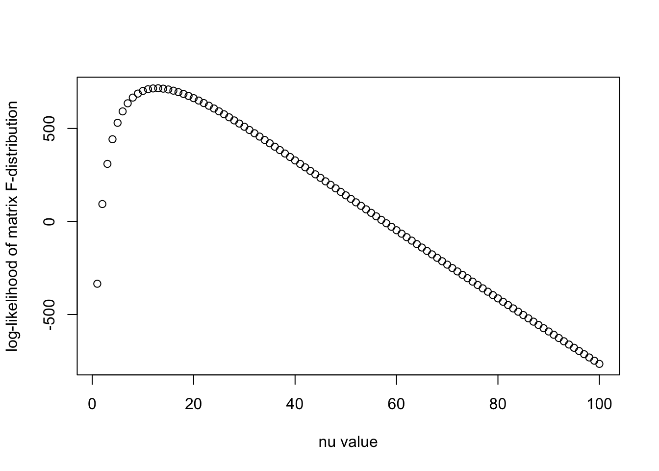
print(paste0("Optimal nu is ", nu_vec[which.max(llhs)]))[1] "Optimal nu is 13"This is slightly better than the Inverse-Wishart distribution, since \(\log |I + N R (R') / \nu|\) behaves better than the trace term \(\mathrm{Trace}(R^{-1} R')\) (log is smaller than linear). However this \(\nu\) is still quite smaller than the out-of-sample size ~300. After the optimal \(\nu\), the likelihood again decreases linearly when \(\nu\) increases.
Now let us try the second model: \(R | \Psi \sim \mathcal{W}(\Psi / N, N)\) and \(\Psi | \Psi' \sim \mathcal{IW}(\nu Psi', \nu + p + 1)\). We have
\[R | \Psi' \sim \mathrm{F}\left(\dfrac{\nu}{N} \Psi', N, \nu + 2\right), \] where \(\Psi'\) is the out-of-sample population covariance matrix. This model feels more natural to me since modeling the in-sample population matrix \(\Psi\) using the out-of-sample population covariance matrix \(\Psi'\) seems more reasonable than using the out-of-sample covariance matrix \(R'\).
In the following we consider two choices of \(\Psi'\) by using (1) PPCA and (2) posterior mean of a Bayesian procedure, then evaluate the matrix F-distribution likelihood.
## Using PPCA to learn Psi' and then plot R, R' and Psi'

eig <- eigen(Rp)
eig_cumsum = cumsum(eig$values)
percent_explained = .999
eig_cumsum = cumsum(eig$values)
q = sum(eig_cumsum < percent_explained * eig_cumsum[p])
sprintf("%d first principle components explain %.1f percent of variance", q, percent_explained*100)
[1] "38 first principle components explain 99.9 percent of variance"## PPCA
lambda <- eig$values
U <- eig$vectors
sigma2_est <- mean(lambda[(q+1):p])
L_diag <- sqrt(lambda[1:q] - sigma2_est)
# L_diag <- sqrt(lambda[1:q])
W_ppca <- U[,1:q] %*% diag(L_diag)
Psi_est <- W_ppca %*% t(W_ppca) + sigma2_est * diag(p)
# Vp = eig$vectors[, c(1:q)]
# Dp = diag(eig$values[c(1:q)])
# Psi_est = Vp %*% Dp %*% t(Vp) + diag(p) * sum(eig$values[c(q + 1, p)])
df3 <- melt(Psi_est)
p3 <- ggplot(df3, aes(Var1, Var2, fill = value)) +
geom_tile() +
scale_fill_gradient2(low="blue", mid="white", high="red") +
coord_fixed() +
ggtitle(paste0("PPCA estimate population cov."))
grid.arrange(p1, p2, p3, ncol = 3)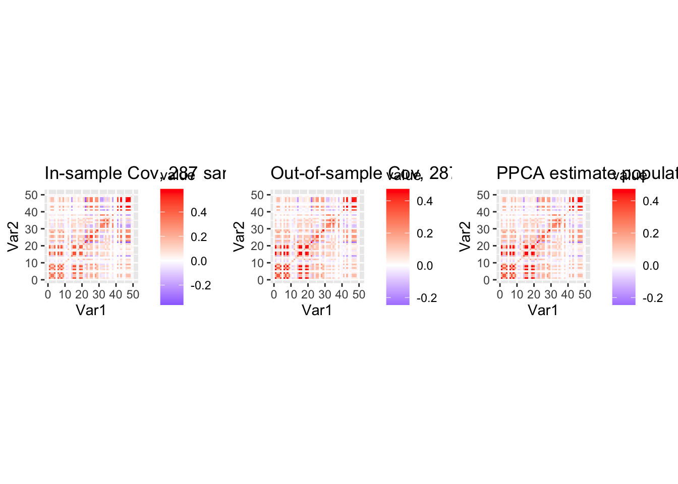
N = nrow(X_in)
nu_vec = c(1:100)
llhs = log_F(R0, Psi_est, N, nu_vec)
plot(nu_vec, llhs, xlab = "nu value", ylab = "log-likelihood of matrix F-distribution")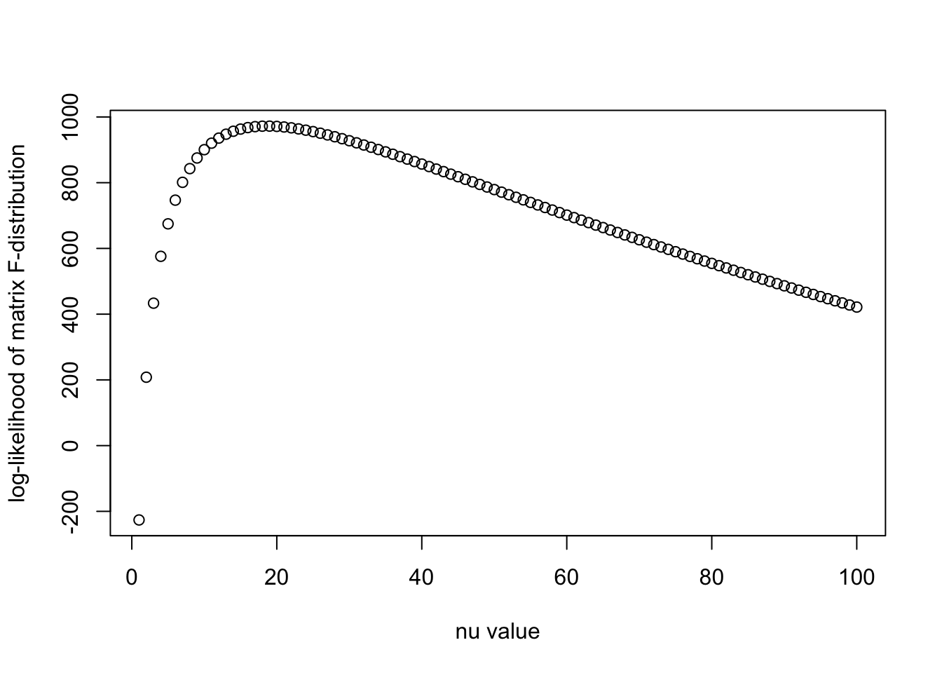
print(paste0("Optimal nu is ", nu_vec[which.max(llhs)]))[1] "Optimal nu is 19"Now let us try the Bayesian estimate: For the uninformative prior \(\Psi' \sim \mathcal{IW}(I, p)\) and \(X'_1, \dots, X'_{N'} \sim N(0, \Psi')\), we have \(\Psi' | X' \sim \mathcal{IW}(N' R' + I, N' + p)\), having the posterior mean \(\dfrac{N'R' + I}{N' - 1}\)
Np = nrow(X_out)
Psi_Bayes <- (Np * Rp + diag(p)) / (Np - 1)


N = nrow(X_in)
nu_vec = c(1:100)
llhs = log_F(R0, Psi_Bayes, N, nu_vec)
plot(nu_vec, llhs, xlab = "nu value", ylab = "log-likelihood of matrix F-distribution")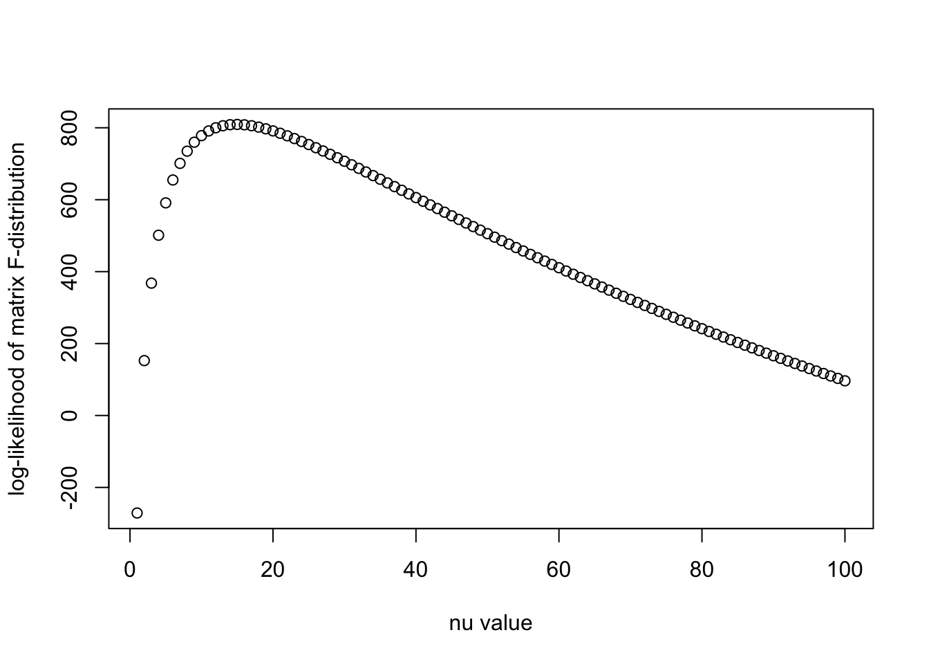
| Version | Author | Date |
|---|---|---|
| fc2f9c8 | dodat | 2025-12-02 |
print(paste0("Optimal nu is ", nu_vec[which.max(llhs)]))[1] "Optimal nu is 15"eig <- eigen(R0)
lambda <- eig$values
U <- eig$vectors
sigma2_est <- mean(lambda[(q+1):p])
L_diag <- sqrt(lambda[1:q] - sigma2_est)
# L_diag <- sqrt(lambda[1:q])
W_ppca <- U[,1:q] %*% diag(L_diag)
Psi <- W_ppca %*% t(W_ppca) + sigma2_est * diag(p)
nu_vec = c(1:100)
# llhs = log_F(Psi, Psi_est, N, nu_vec)
llhs = log_iw(Psi, Psi_est, nu_vec)
plot(nu_vec, llhs, xlab = "nu value", ylab = "log-likelihood of matrix F-distribution")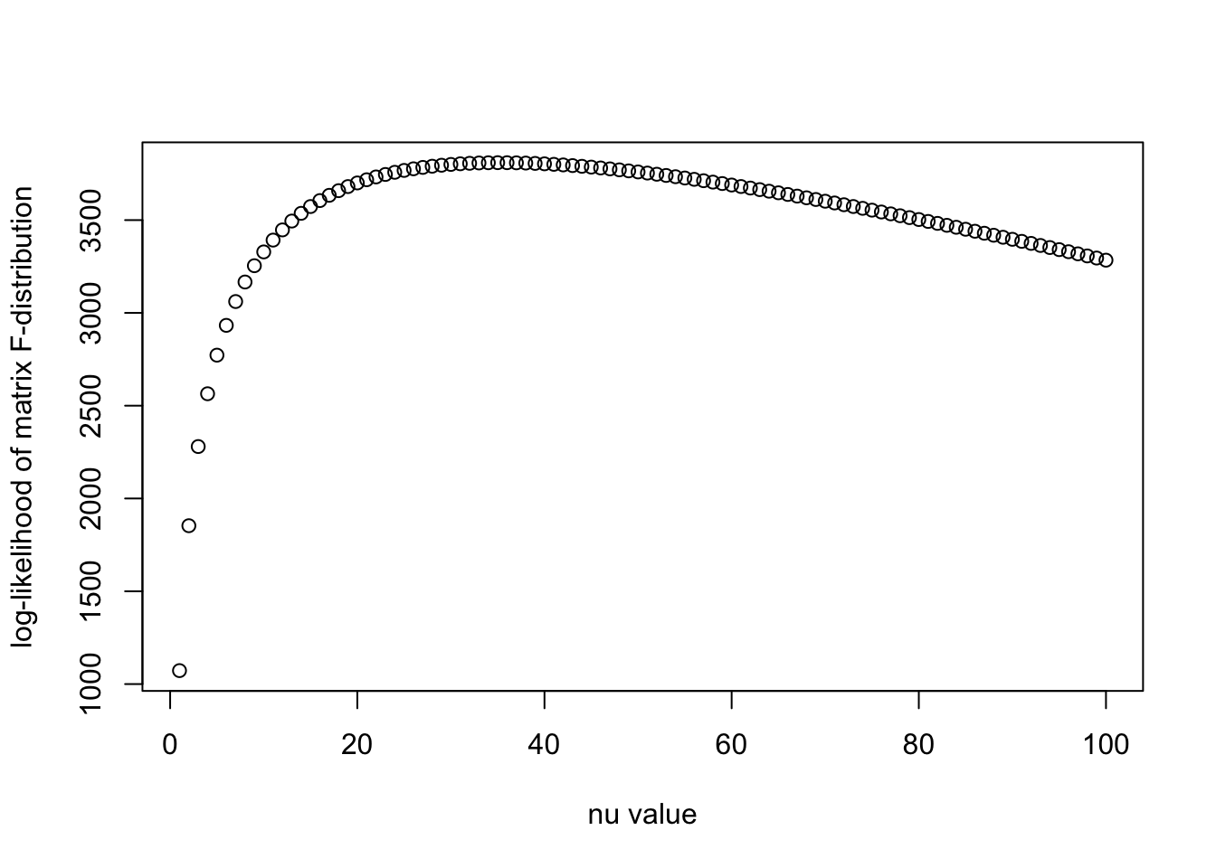
| Version | Author | Date |
|---|---|---|
| d3b0e4f | dodat97 | 2025-12-02 |
print(paste0("Optimal nu is ", nu_vec[which.max(llhs)]))[1] "Optimal nu is 35"I have no idea why only when we optimize \(\nu\) in the likelihood of \(p(\Psi | \Psi')\) we have a good estimate of \(\nu\). Although the model \[\Psi | \Psi' \sim \mathcal{IW}(\nu \Psi', \nu + p + 1)\] is equivalent to \[R | \Psi' \sim \mathrm{F}(\frac{\nu \Psi'}{N}, N, \nu + 2). \]
One explanation is that even the model \(X_1, \dots, X_N \sim N(0, \Psi)\) is mis-specified.
There are four players here: The sample covariance matrices \(R, R'\) and population covariance matrix \(\Psi, \Psi'\). We need to have a smart model for them.
Another strategy is to model the eigen-decomposition of \(R\), i.e., its eigenvalues and vectors. It looks like the low-rank is still a problem.
sessionInfo()R version 4.5.1 (2025-06-13)
Platform: aarch64-apple-darwin20
Running under: macOS Sequoia 15.0
Matrix products: default
BLAS: /Library/Frameworks/R.framework/Versions/4.5-arm64/Resources/lib/libRblas.0.dylib
LAPACK: /Library/Frameworks/R.framework/Versions/4.5-arm64/Resources/lib/libRlapack.dylib; LAPACK version 3.12.1
locale:
[1] en_US.UTF-8/en_US.UTF-8/en_US.UTF-8/C/en_US.UTF-8/en_US.UTF-8
time zone: America/Chicago
tzcode source: internal
attached base packages:
[1] stats graphics grDevices utils datasets methods base
other attached packages:
[1] gridExtra_2.3 reshape2_1.4.4 ggplot2_3.5.2 Matrix_1.7-3
[5] susieR_0.14.2 workflowr_1.7.2
loaded via a namespace (and not attached):
[1] sass_0.4.10 stringi_1.8.7 lattice_0.22-7 digest_0.6.37
[5] magrittr_2.0.3 evaluate_1.0.5 grid_4.5.1 RColorBrewer_1.1-3
[9] fastmap_1.2.0 rprojroot_2.1.1 plyr_1.8.9 jsonlite_2.0.0
[13] processx_3.8.6 whisker_0.4.1 reshape_0.8.10 ps_1.9.1
[17] mixsqp_0.3-54 promises_1.5.0 httr_1.4.7 scales_1.4.0
[21] jquerylib_0.1.4 cli_3.6.5 rlang_1.1.6 crayon_1.5.3
[25] withr_3.0.2 cachem_1.1.0 yaml_2.3.10 otel_0.2.0
[29] tools_4.5.1 httpuv_1.6.16 vctrs_0.6.5 R6_2.6.1
[33] matrixStats_1.5.0 lifecycle_1.0.4 git2r_0.36.2 stringr_1.5.2
[37] fs_1.6.6 irlba_2.3.5.1 pkgconfig_2.0.3 callr_3.7.6
[41] pillar_1.11.0 bslib_0.9.0 later_1.4.4 gtable_0.3.6
[45] glue_1.8.0 Rcpp_1.1.0 xfun_0.53 tibble_3.3.0
[49] rstudioapi_0.17.1 knitr_1.50 farver_2.1.2 htmltools_0.5.8.1
[53] labeling_0.4.3 rmarkdown_2.29 compiler_4.5.1 getPass_0.2-4