Investigate V after every iteration in SuSiE RSS
Dat Do
2025-09-08
Last updated: 2025-09-10
Checks: 7 0
Knit directory: Improved_LD_SuSiE/
This reproducible R Markdown analysis was created with workflowr (version 1.7.1). The Checks tab describes the reproducibility checks that were applied when the results were created. The Past versions tab lists the development history.
Great! Since the R Markdown file has been committed to the Git repository, you know the exact version of the code that produced these results.
Great job! The global environment was empty. Objects defined in the global environment can affect the analysis in your R Markdown file in unknown ways. For reproduciblity it’s best to always run the code in an empty environment.
The command set.seed(20250821) was run prior to running
the code in the R Markdown file. Setting a seed ensures that any results
that rely on randomness, e.g. subsampling or permutations, are
reproducible.
Great job! Recording the operating system, R version, and package versions is critical for reproducibility.
Nice! There were no cached chunks for this analysis, so you can be confident that you successfully produced the results during this run.
Great job! Using relative paths to the files within your workflowr project makes it easier to run your code on other machines.
Great! You are using Git for version control. Tracking code development and connecting the code version to the results is critical for reproducibility.
The results in this page were generated with repository version b06d838. See the Past versions tab to see a history of the changes made to the R Markdown and HTML files.
Note that you need to be careful to ensure that all relevant files for
the analysis have been committed to Git prior to generating the results
(you can use wflow_publish or
wflow_git_commit). workflowr only checks the R Markdown
file, but you know if there are other scripts or data files that it
depends on. Below is the status of the Git repository when the results
were generated:
Ignored files:
    Ignored:    .DS_Store
    Ignored:    .Rhistory
    Ignored:    .Rproj.user/
    Ignored:    analysis/.Rhistory
    Ignored:    code/.DS_Store
    Ignored:    output/.DS_Store

Untracked files:
    Untracked:  code/Interpolate-idea.R
    Untracked:  code/R_algorithm_test.R
    Untracked:  code/R_algorithms.R
    Untracked:  code/SuSiE_rss.R
    Untracked:  code/SuSiE_rss_multi_SNPs.R
    Untracked:  code/SuSiE_rss_test.R
    Untracked:  code/compare_LD_mat_Dykstra_fullSVD.R
    Untracked:  code/iterpolate-idea-visualize.R
    Untracked:  code/prototype_R_code.R
    Untracked:  code/test_visualize_many_traits.R
    Untracked:  code/test_visualize_one_trait.R
    Untracked:  code_push.R
    Untracked:  output/compare_LD_Ltrue_1.pdf
    Untracked:  output/compare_LD_Ltrue_2.pdf
    Untracked:  output/coverages_mat_multi_trait.RData
    Untracked:  output/coverages_mat_multi_trait_L1.RData
    Untracked:  output/coverages_mat_multi_trait_L2.RData
    Untracked:  output/number_CSs_mat_multi_trait.RData
    Untracked:  output/number_CSs_mat_multi_trait_L1.RData
    Untracked:  output/number_CSs_mat_multi_trait_L2.RData
    Untracked:  output/number_SNPs_per_CS_mat_multi_trait.RData
    Untracked:  output/number_SNPs_per_CS_mat_multi_trait_L1.RData
    Untracked:  output/number_SNPs_per_CS_mat_multi_trait_L2.RData
    Untracked:  output/powers_mat_multi_trait.RData
    Untracked:  output/powers_mat_multi_trait_L1.RData
    Untracked:  output/powers_mat_multi_trait_L2.RData
Note that any generated files, e.g. HTML, png, CSS, etc., are not included in this status report because it is ok for generated content to have uncommitted changes.
These are the previous versions of the repository in which changes were
made to the R Markdown (analysis/V_xy_iter_investigate.Rmd)
and HTML (docs/V_xy_iter_investigate.html) files. If you’ve
configured a remote Git repository (see ?wflow_git_remote),
click on the hyperlinks in the table below to view the files as they
were in that past version.
| File | Version | Author | Date | Message |
|---|---|---|---|---|
| Rmd | b06d838 | dodat97 | 2025-09-10 | wflow_publish(c("analysis/V_xy_iter_investigate.Rmd")) |
| html | 25b3a8d | dodat97 | 2025-09-09 | Build site. |
| Rmd | cf00a45 | dodat97 | 2025-09-09 | wflow_publish(c("analysis/V_xy_iter_investigate.Rmd")) |
| html | 2f35f45 | dodat97 | 2025-09-09 | Build site. |
| Rmd | 5e0c2a7 | dodat97 | 2025-09-09 | wflow_publish(c("analysis/V_xy_iter_investigate.Rmd")) |
| html | c1960a3 | dodat97 | 2025-09-08 | Build site. |
| Rmd | 0e1cebc | dodat97 | 2025-09-08 | wflow_publish(c("analysis/V_xy_iter_investigate.Rmd")) |
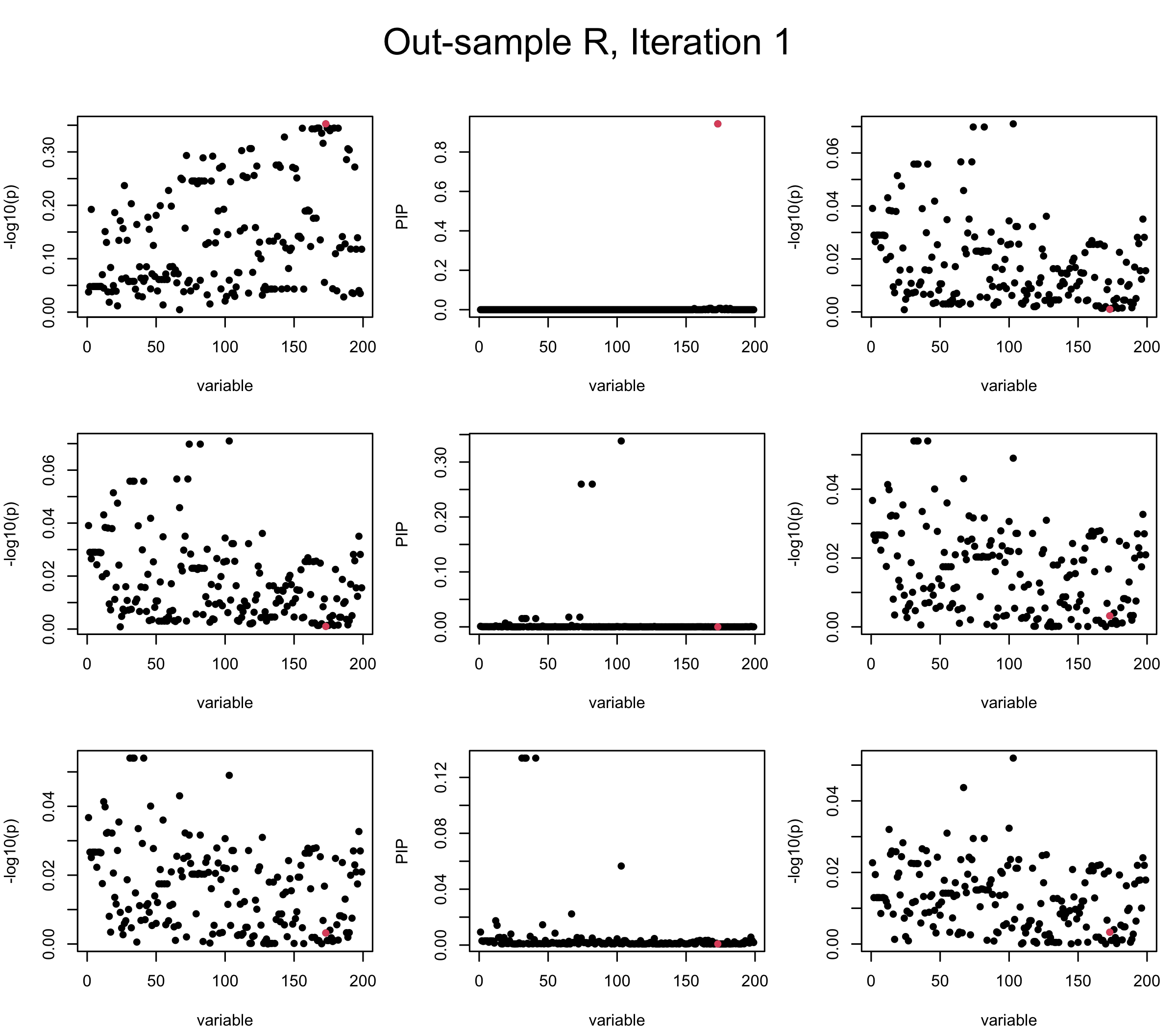
Here we want to investigate why using out-of-sample LD matrix can cause many false discovery by looking that the result after every training iteration. Recall that SuSiE_rss work by iteratively fitting Single Effect Model to the residuals: \[\overline{r} = X^{\top} y - X^{\top} X \overline{b} = v - R \overline{b} \] where \(\overline{b} = \sum_{\ell=1}^{L} \overline{b}_{\ell}\) is the sum of the posterior mean of all effects.
We expect that after detecting all ``true’’ causal SNP, \(\overline{r}\) will be a vector of \(J\) equally small numbers so that the PIP of over-fitted \(\ell\) will be close to 0 (diffused). Hence the purity of over-fitted \(\ell\)-th CS is small and is not reported.
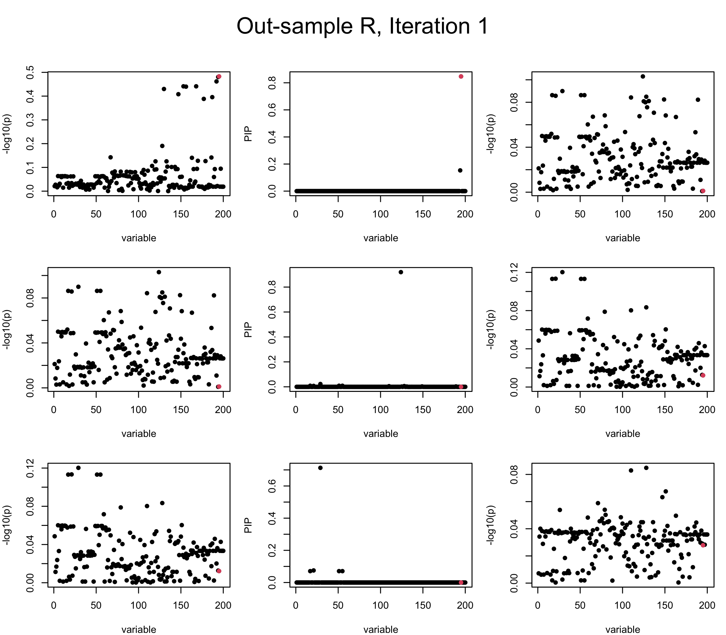
However, it can be seen that because of mis-specified \(R\), after controlling for all causal SNP, the residual \(\overline{r}\) of other SNPs can ``increase’’, leading to large PIP, thus creates false discovery. The second (related) case is that when subtracting \(\widehat{R} \overline{b}\) from \(v\), because of the mismatch between \(\widehat{R}\) and \(R\), some of the correlated SNP to the causal SNP is not subtracted enough. Consider an example: \(v_i = 5, v_j = 6\) and \(R_{ij} \approx 1\), all other \(v_{k}= 0\). After one iteration that SuSiE pick the credible set \(\{i, j\}\), we expect \(\overline{v}_{i} = \overline{v}_j = 0\). However, if \(\widehat{R}_{ij} \ll R_{ij}\), then the PIP of SNP \(i\) in the first CS will be much smaller, leading to smaller subtraction term \(R \overline{b}\), which causes big residual \(\overline{r}_j\).
We will also see that our method (projected \(R\)) will experience the second behavior (not subtracting enough) much less.
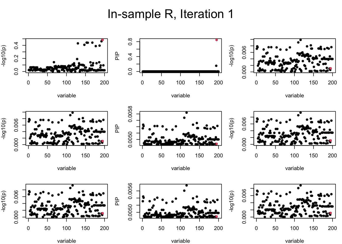
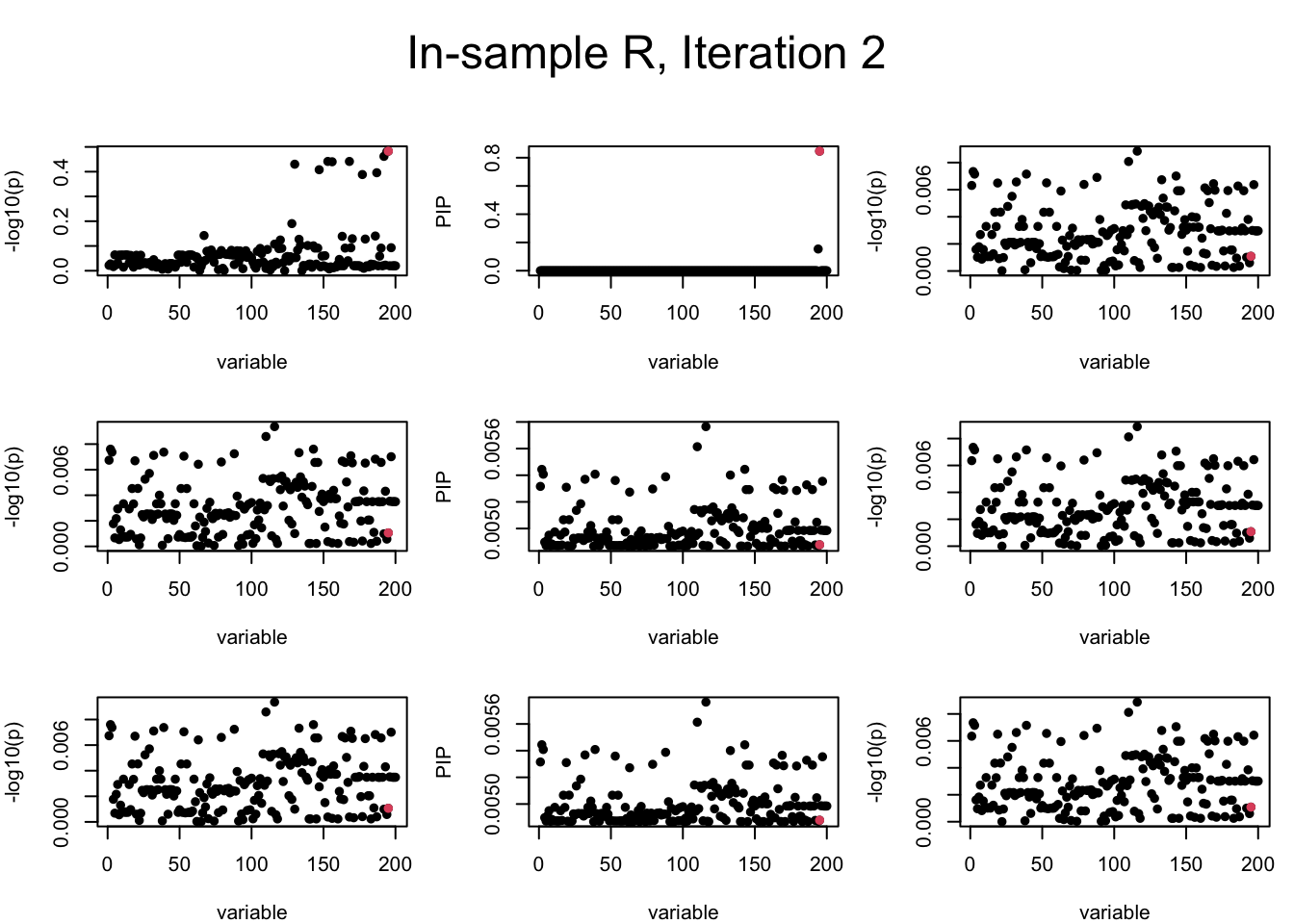
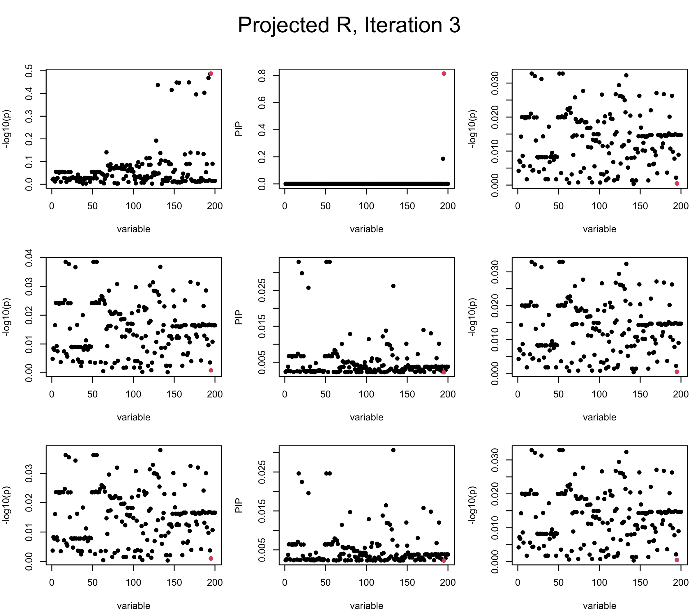
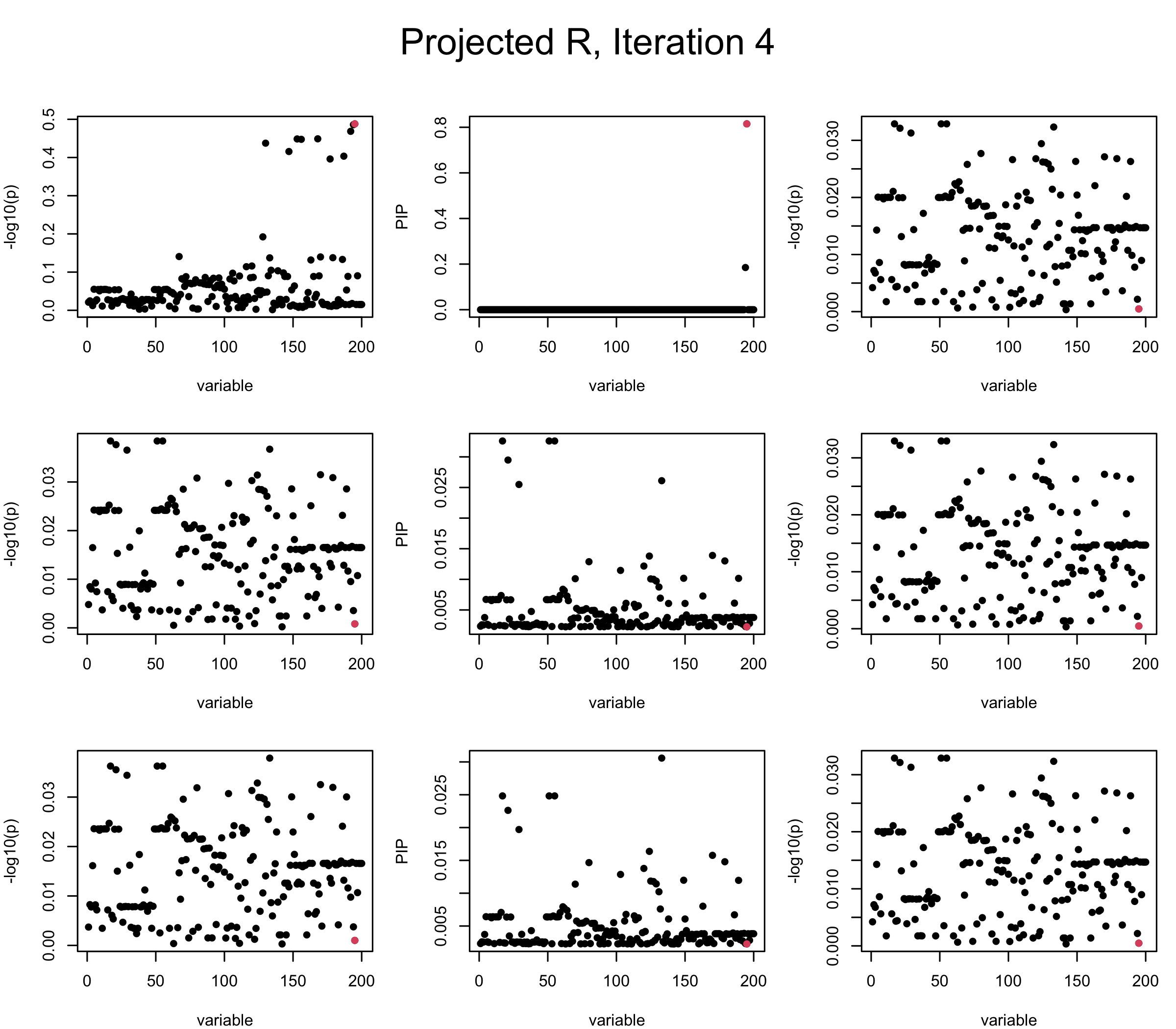
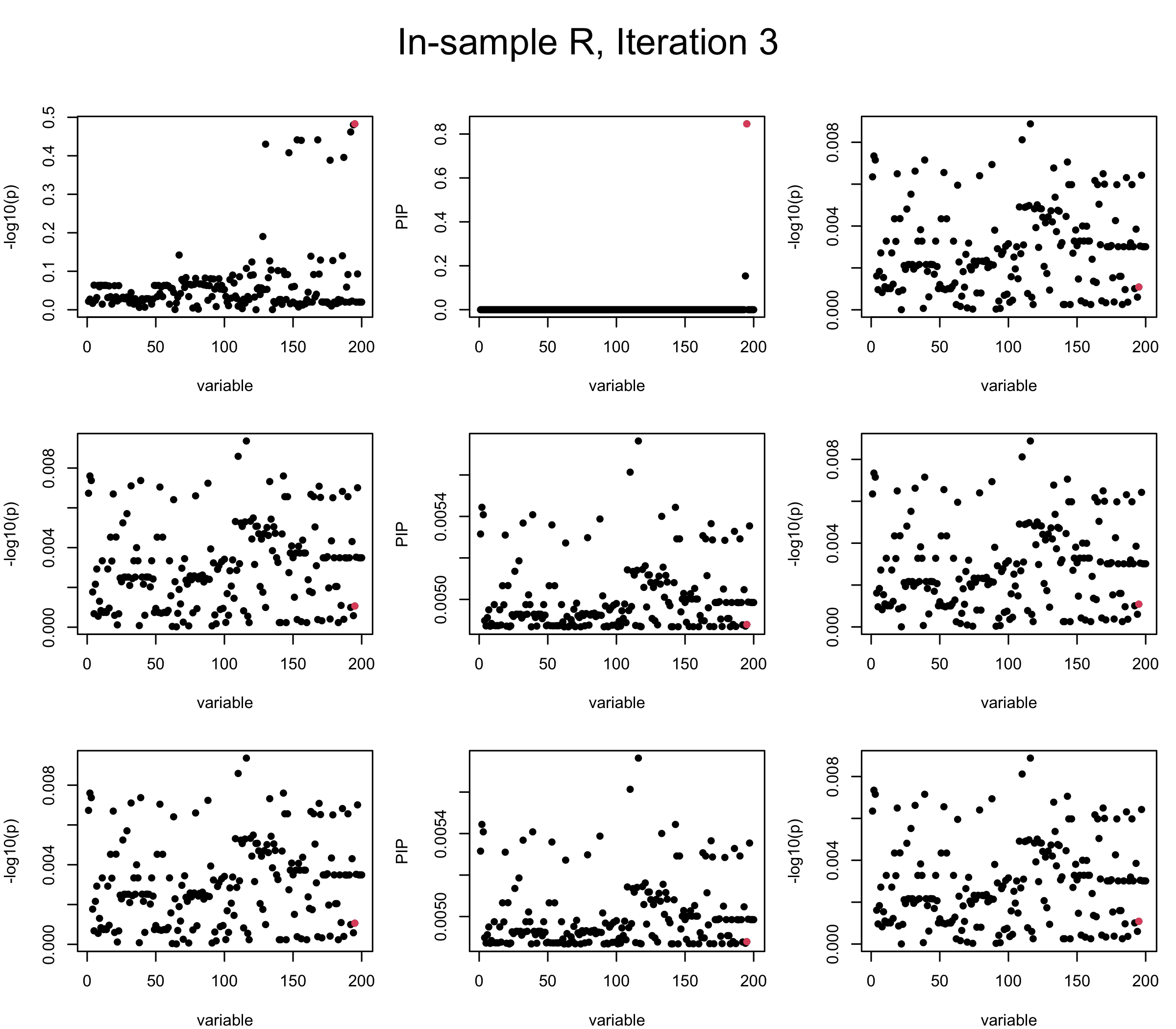
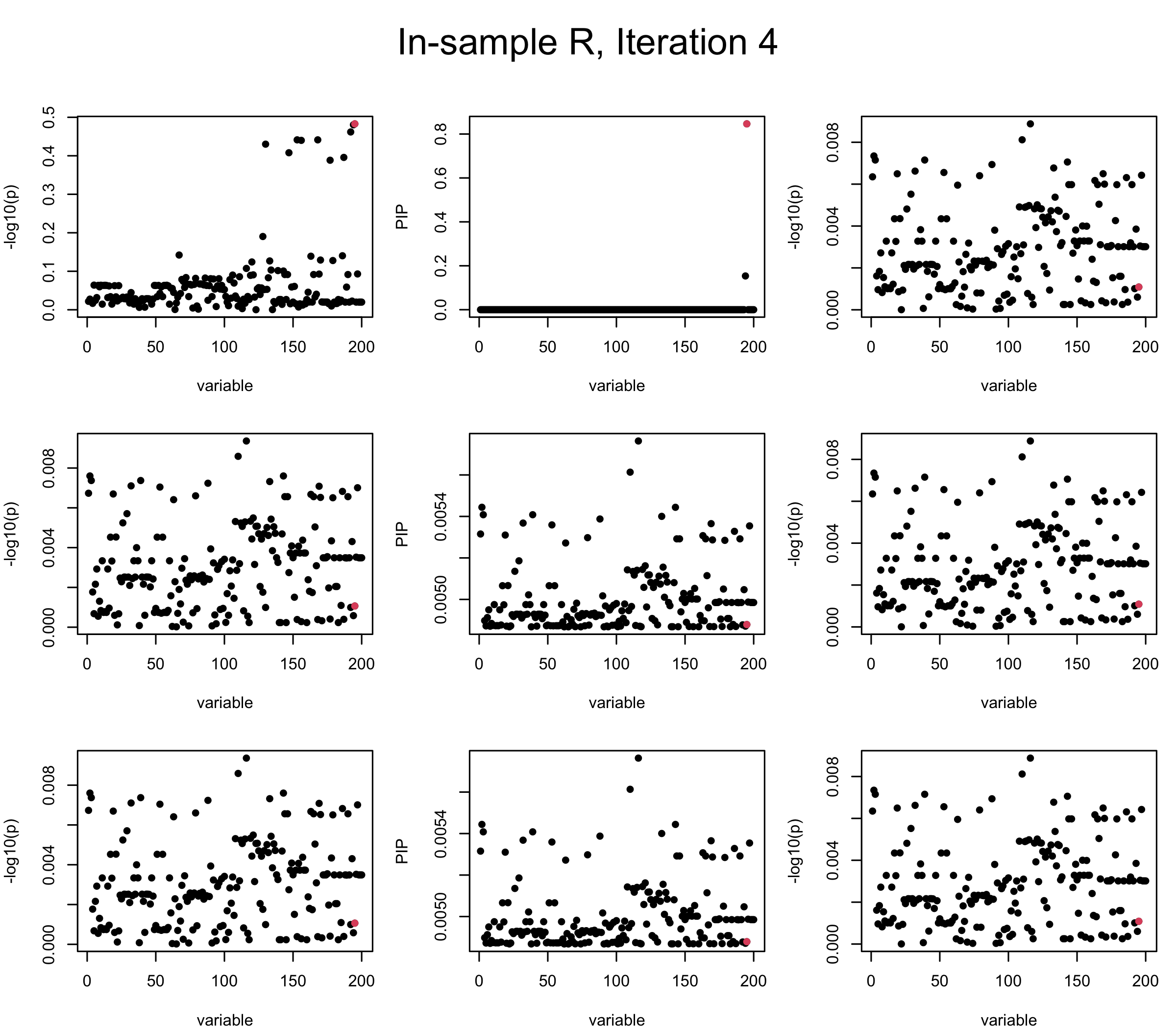
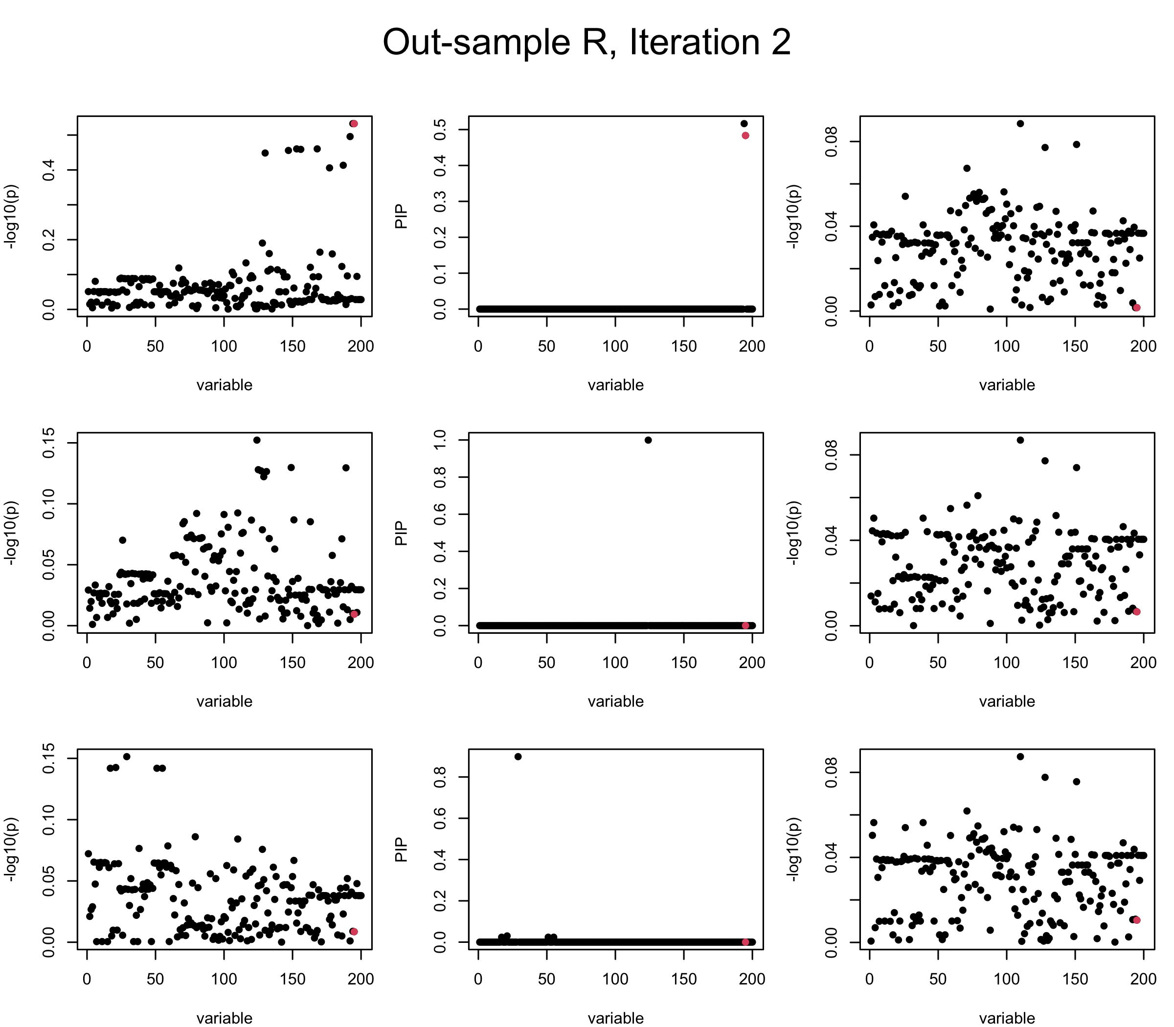
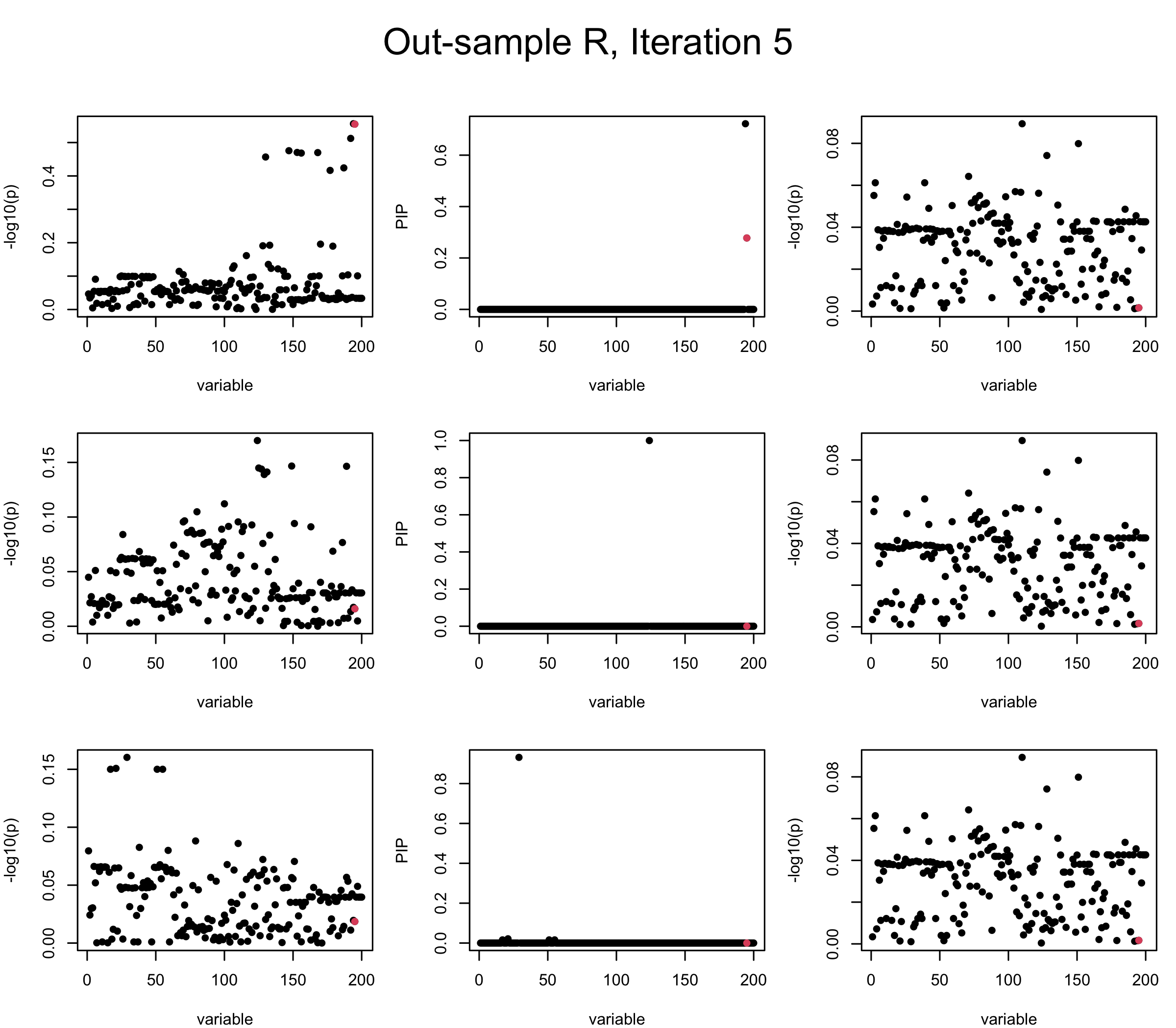
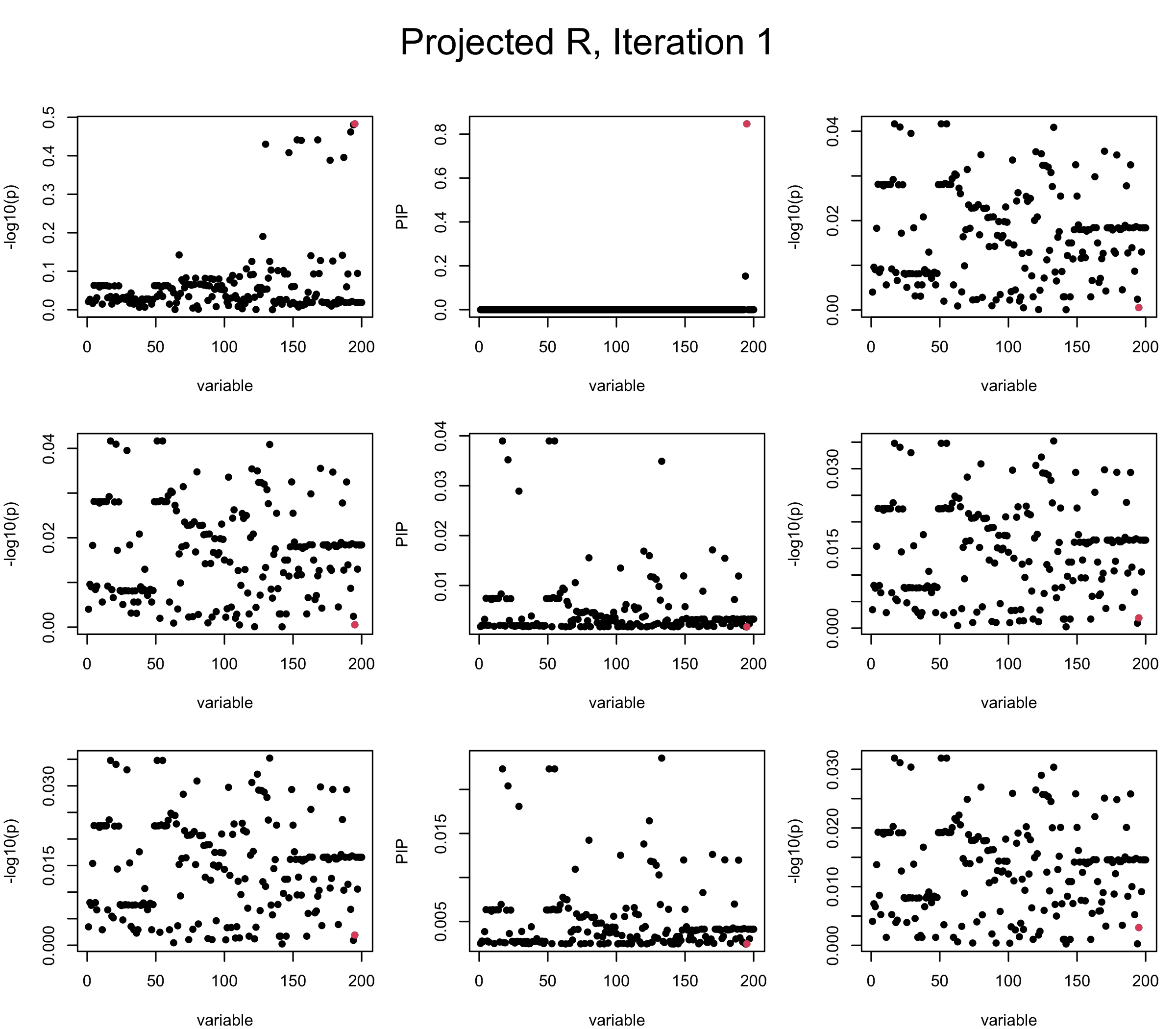
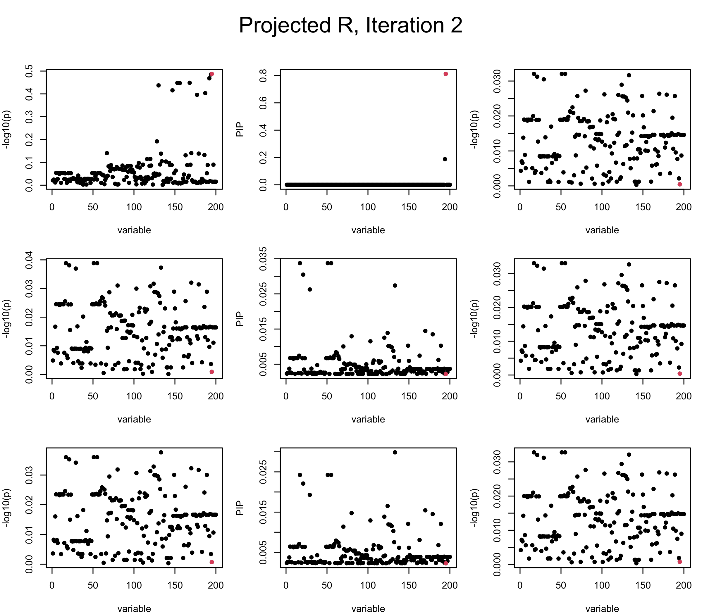
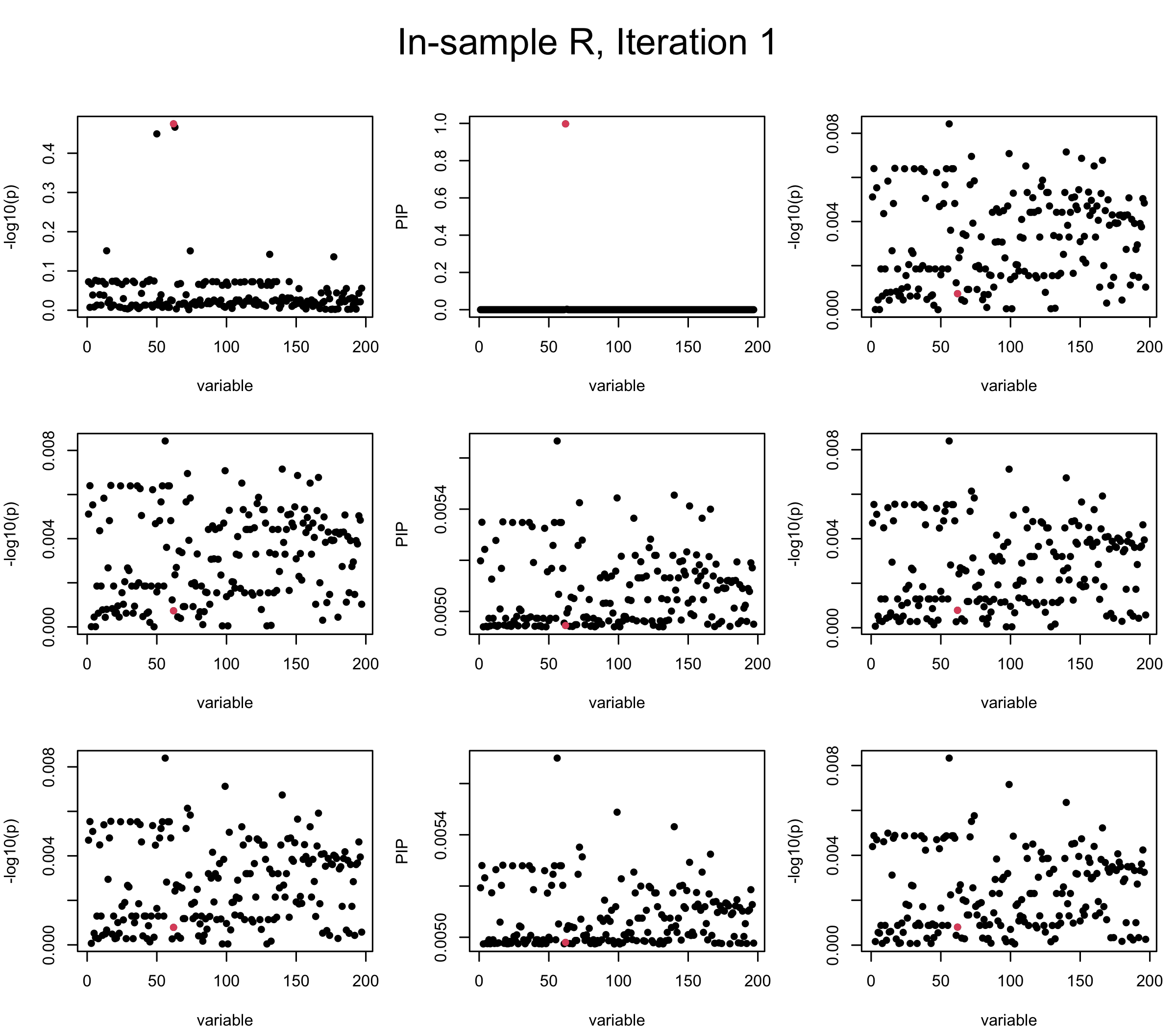
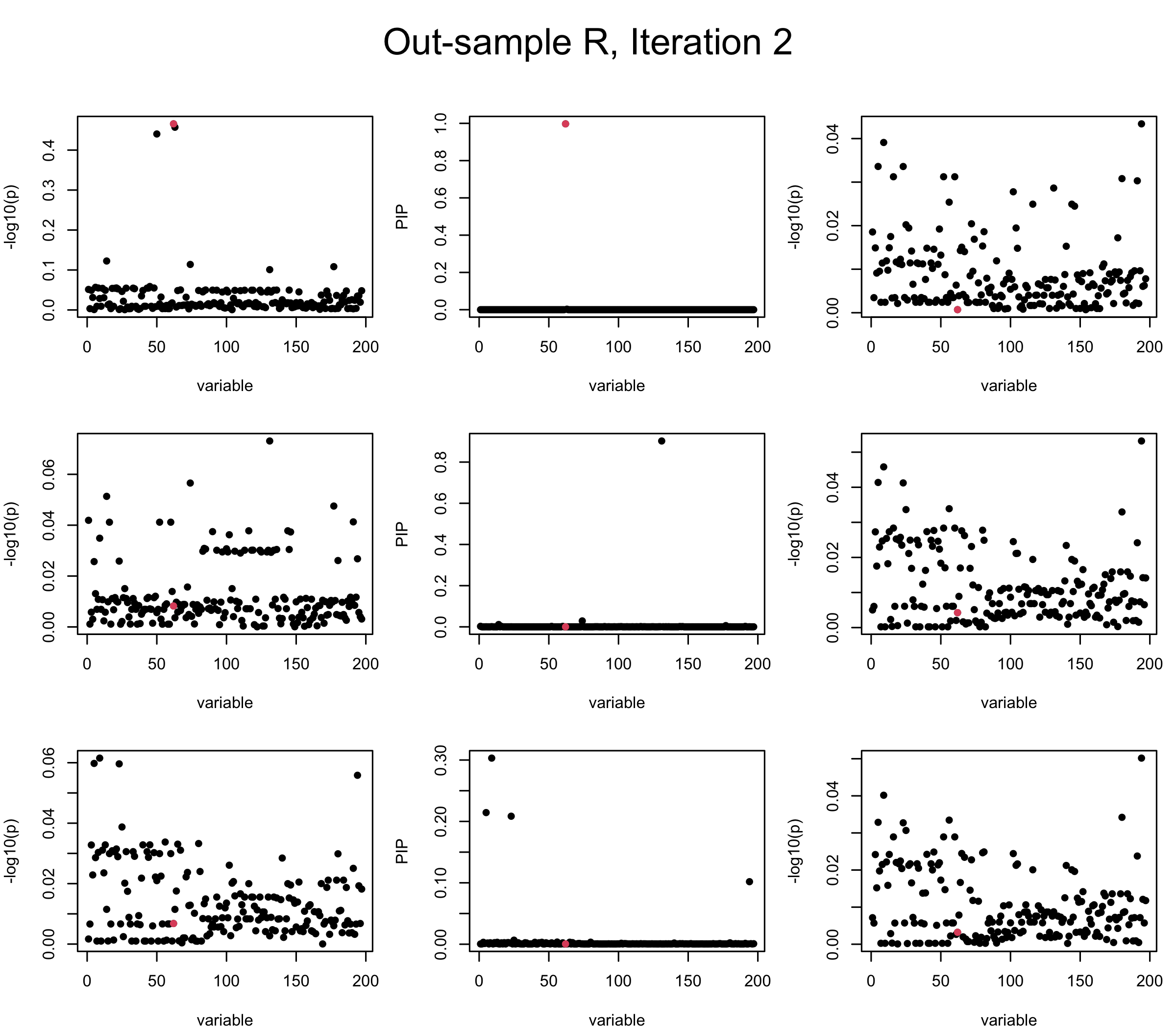
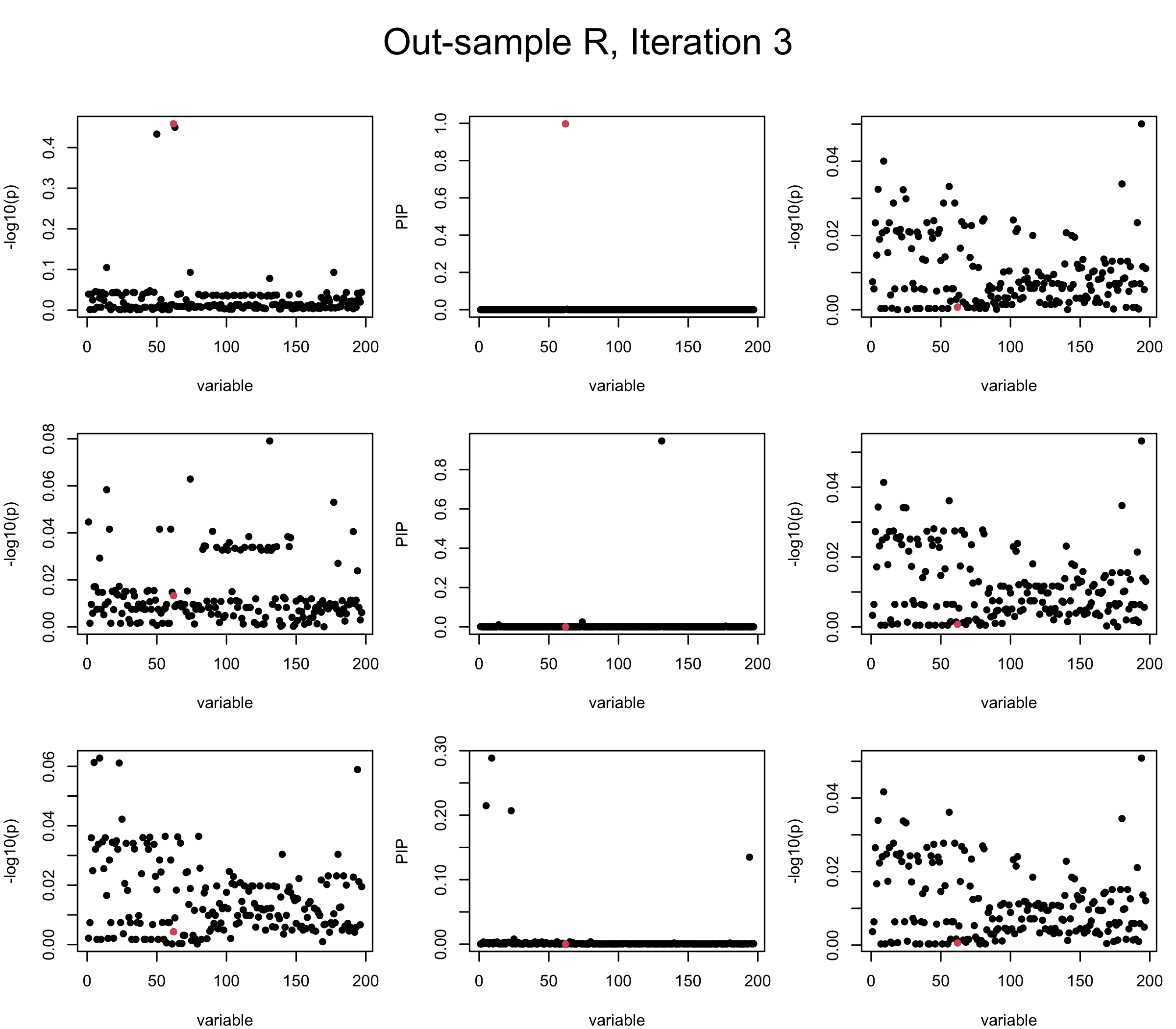
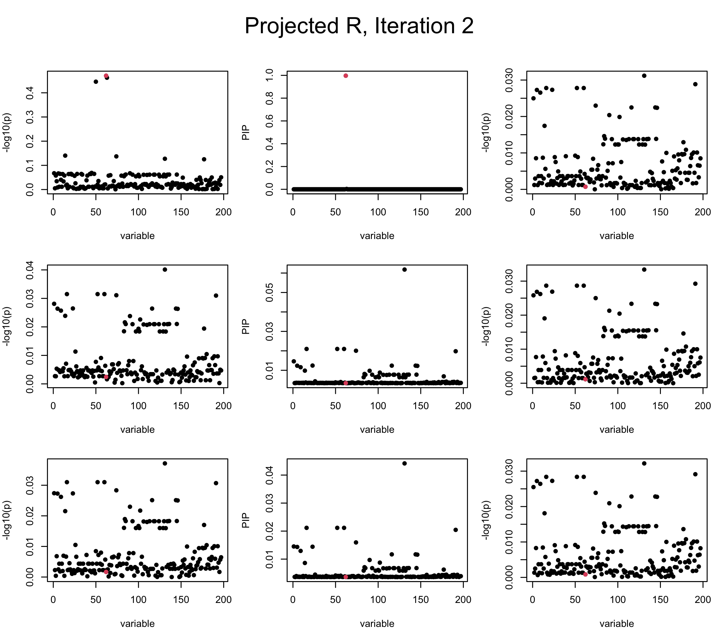
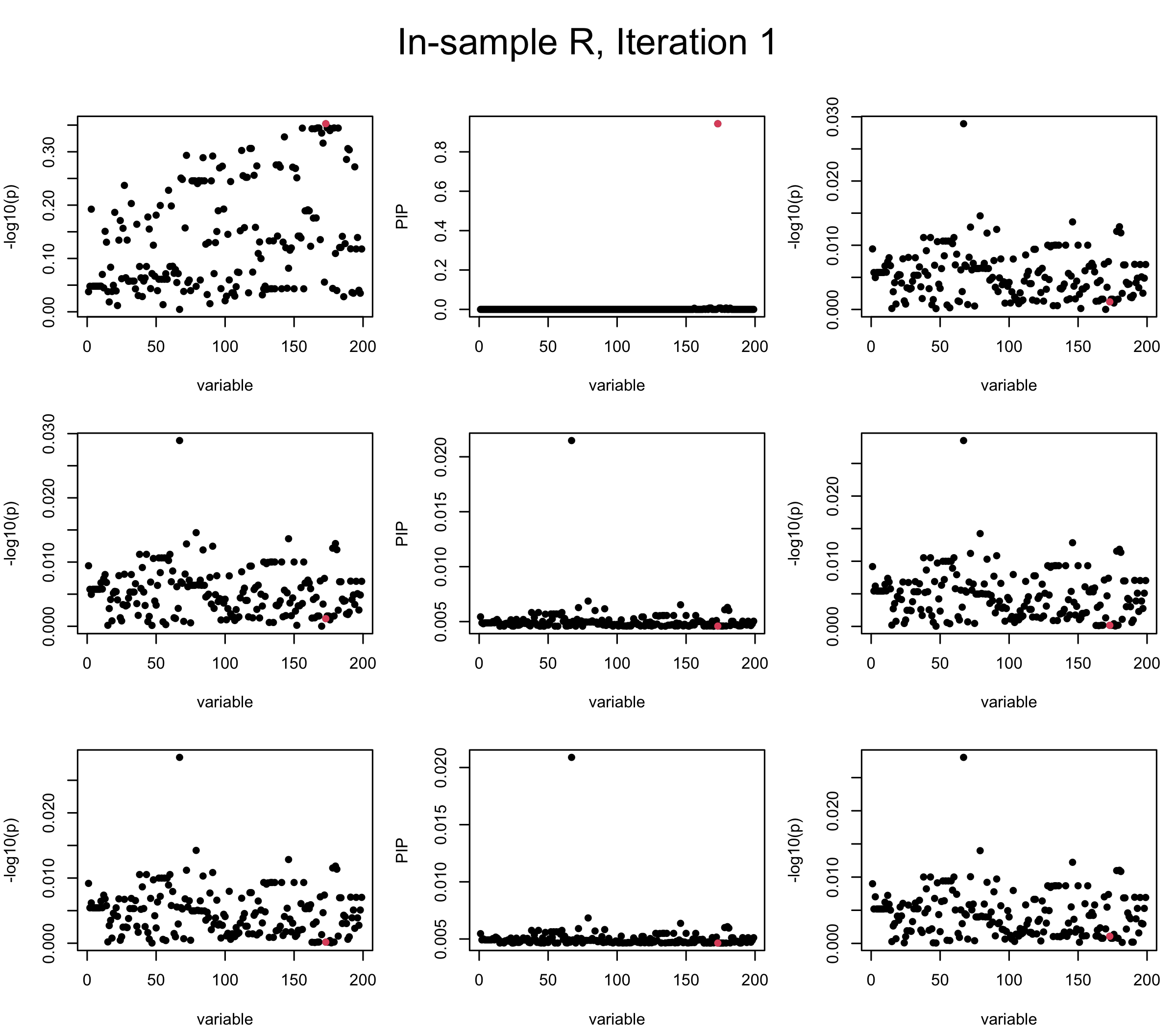
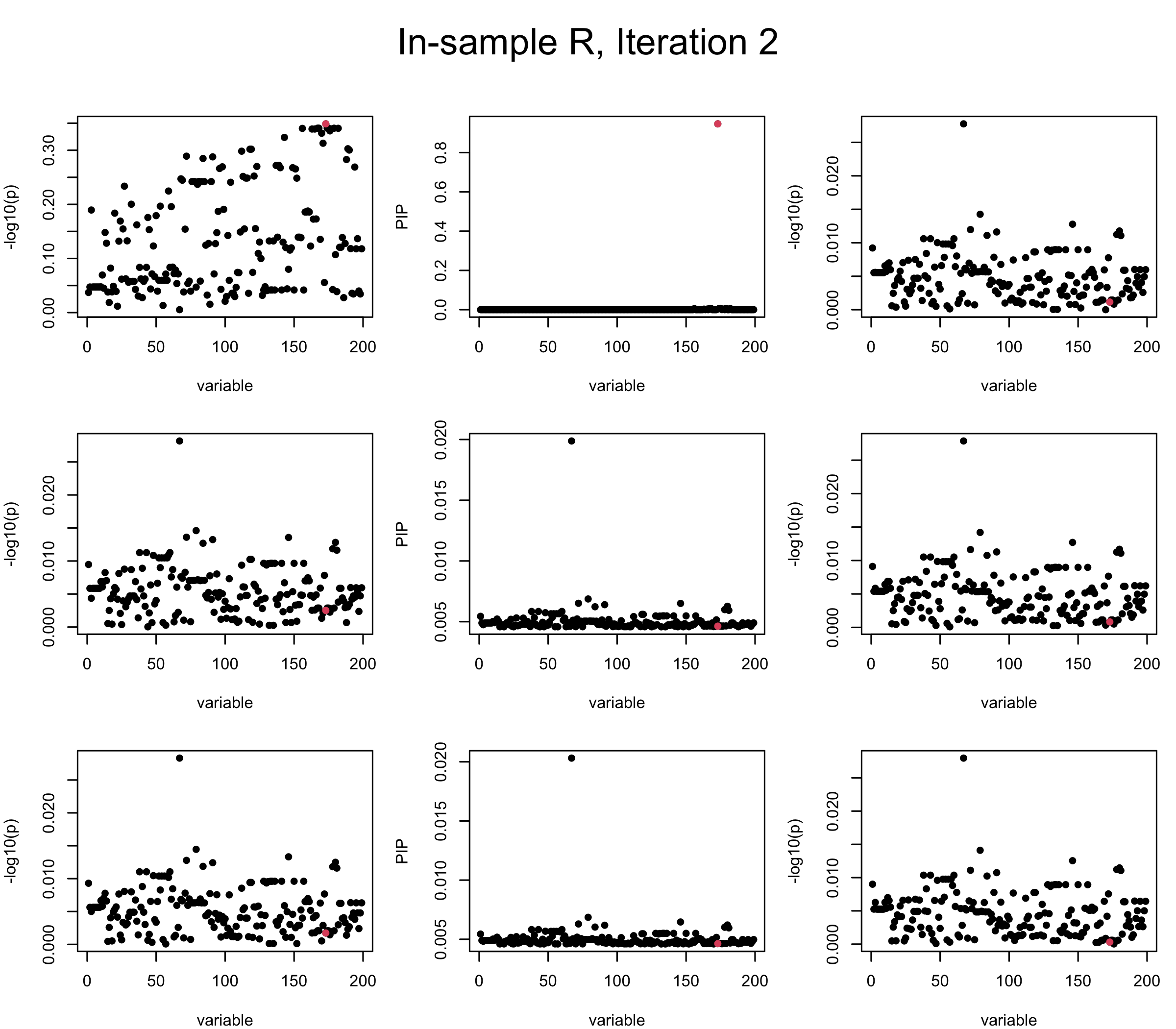
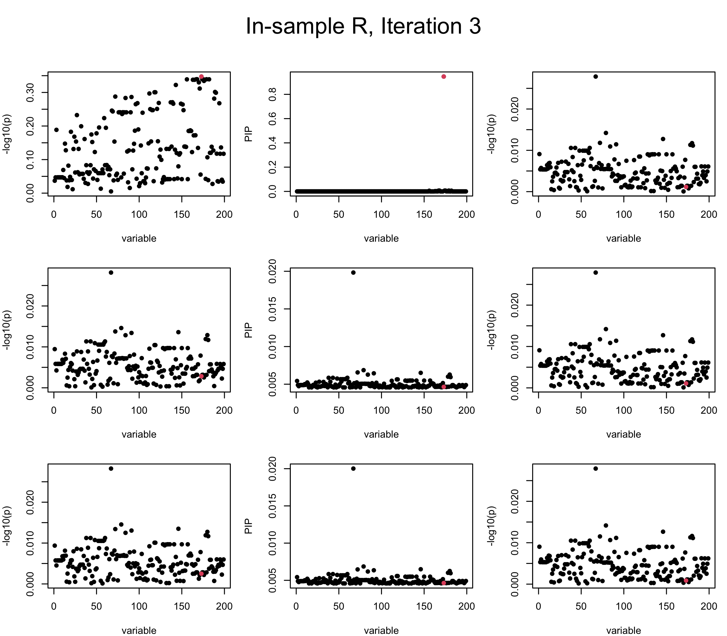
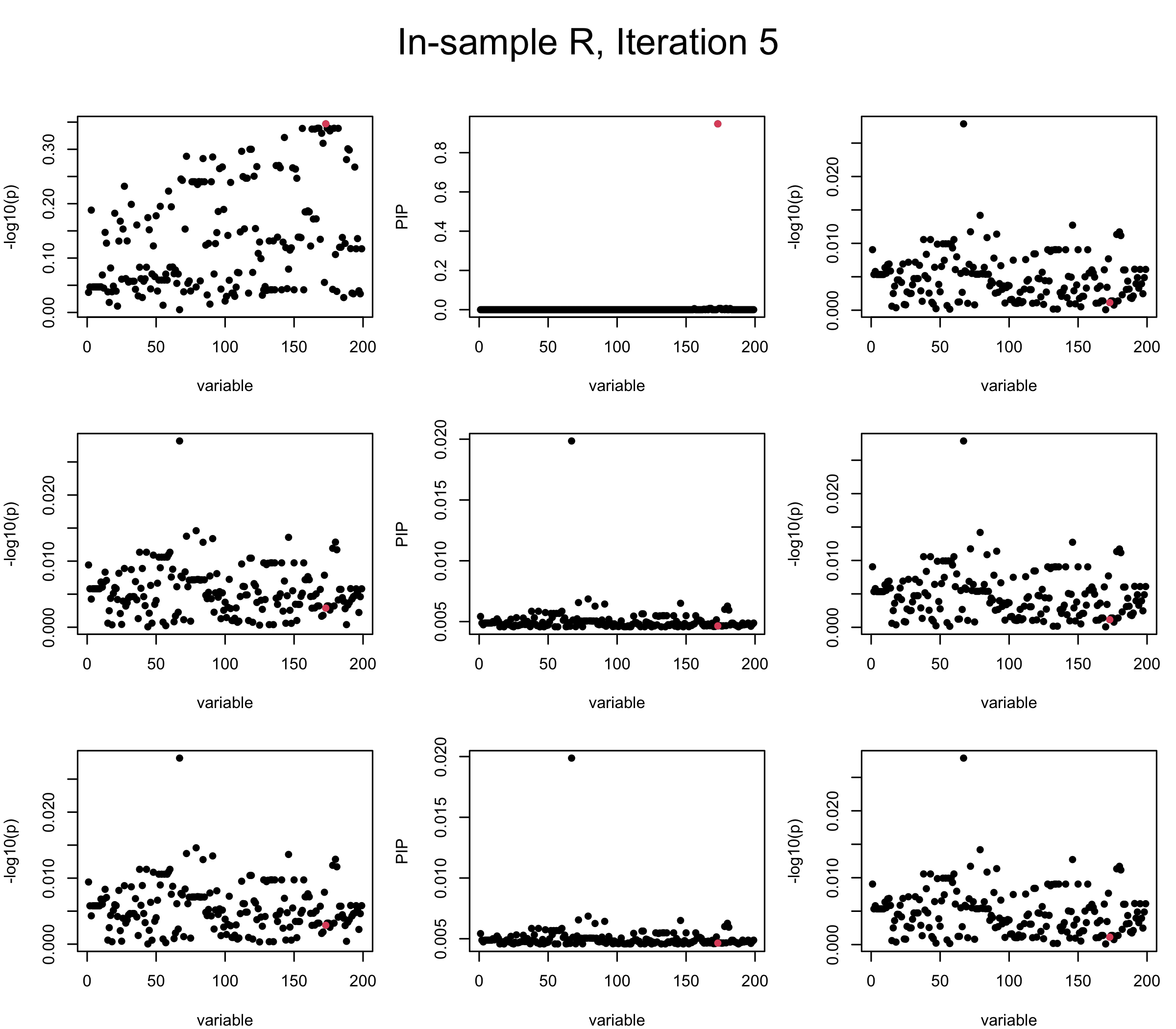
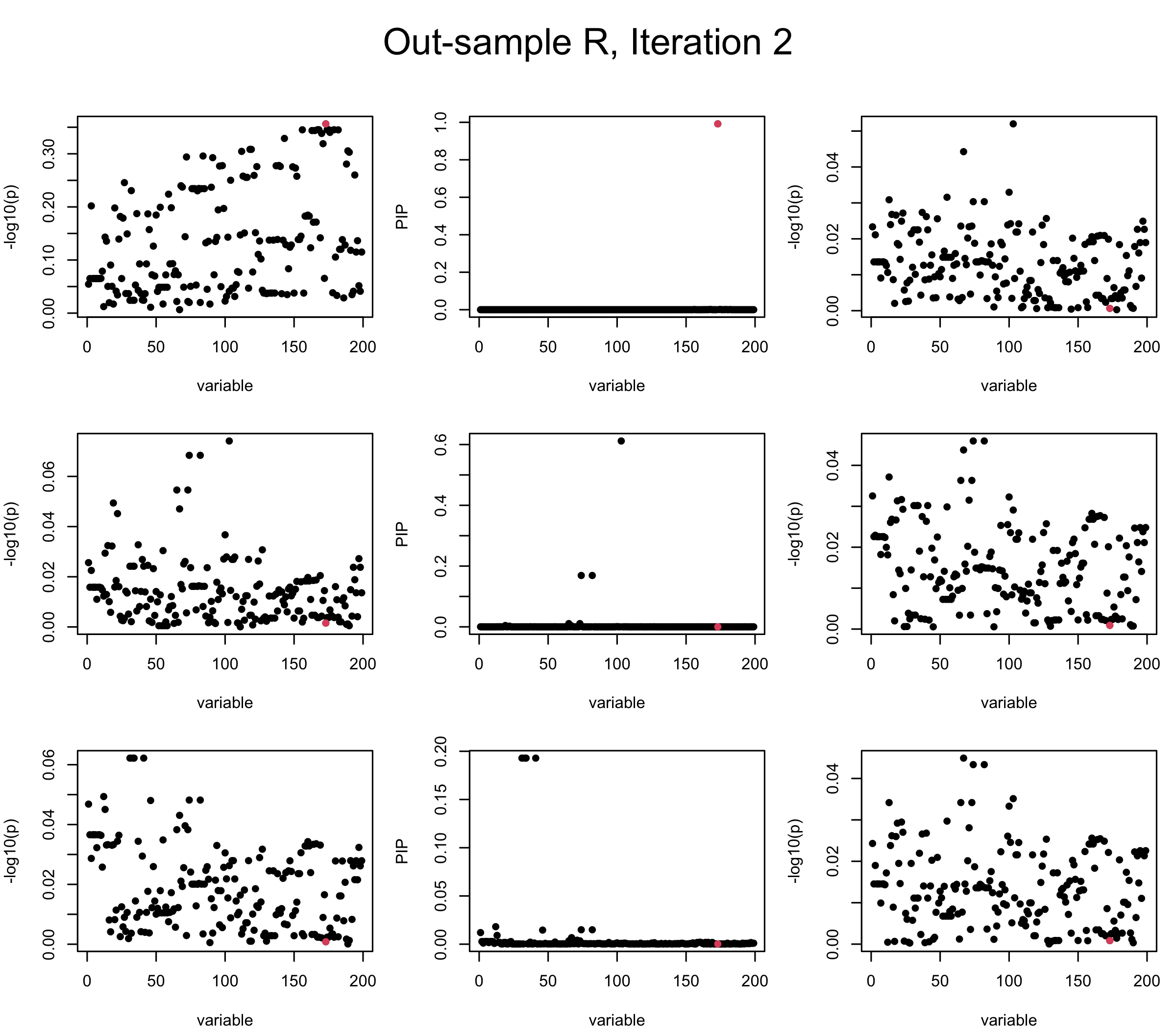
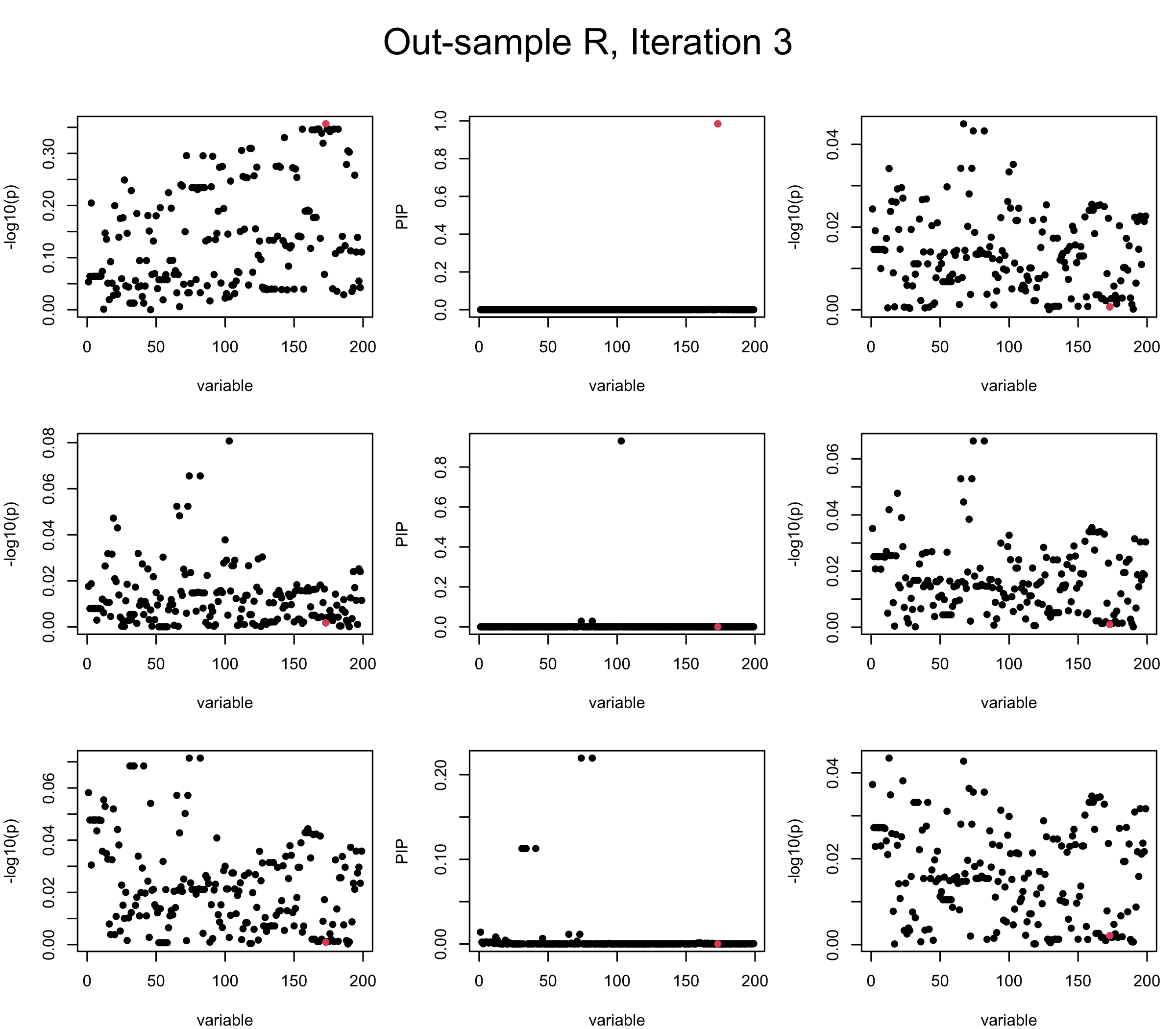
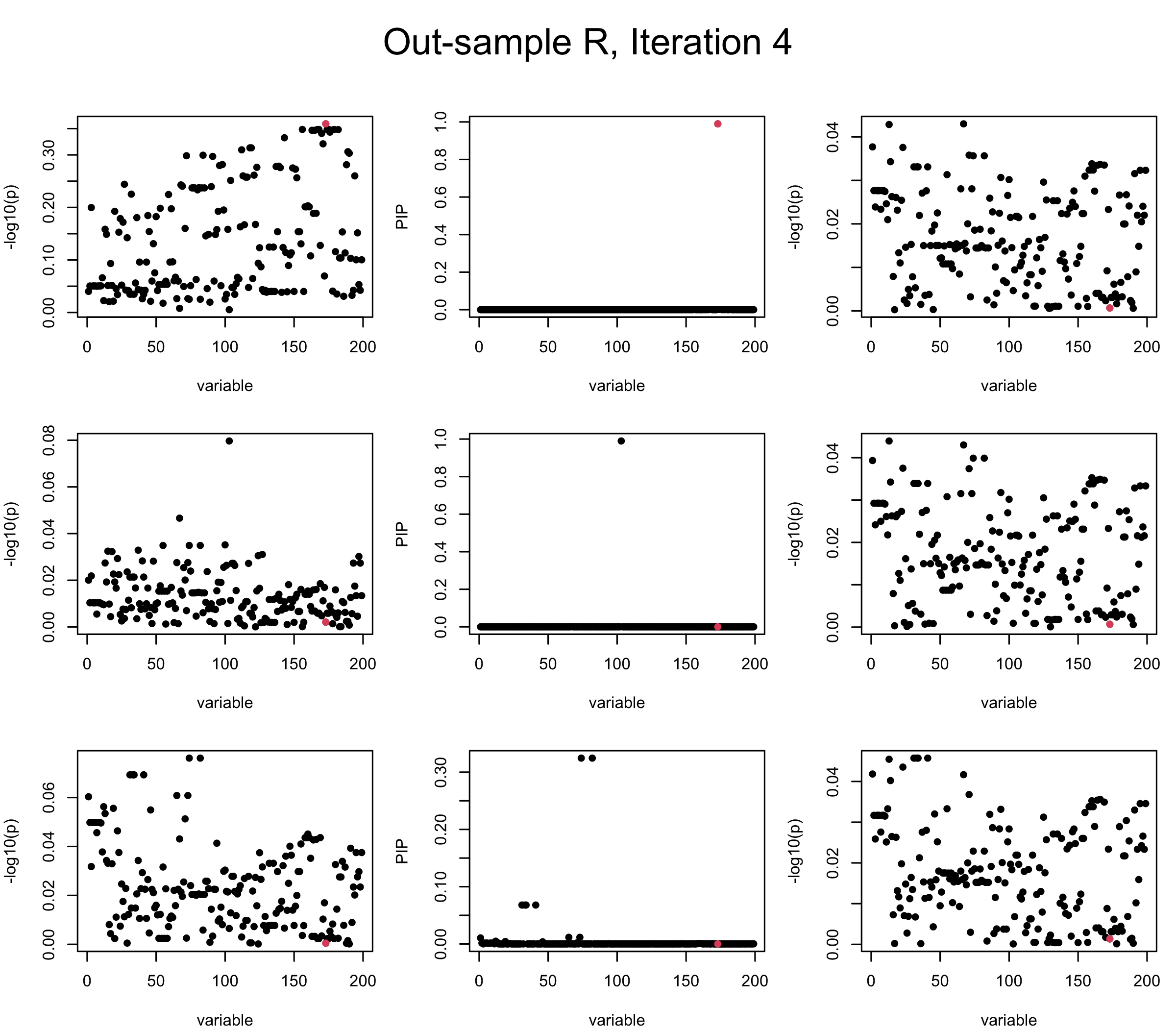
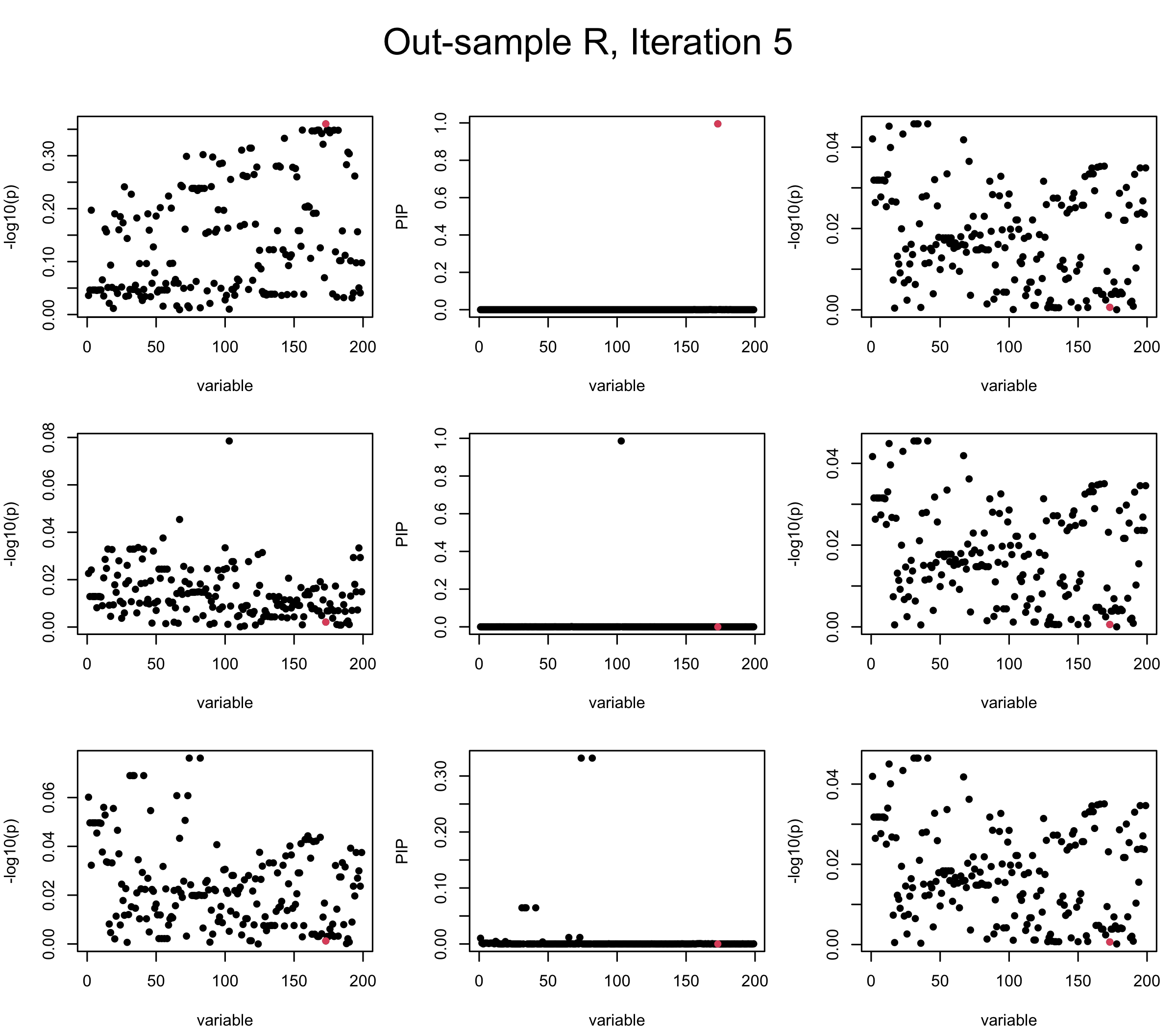
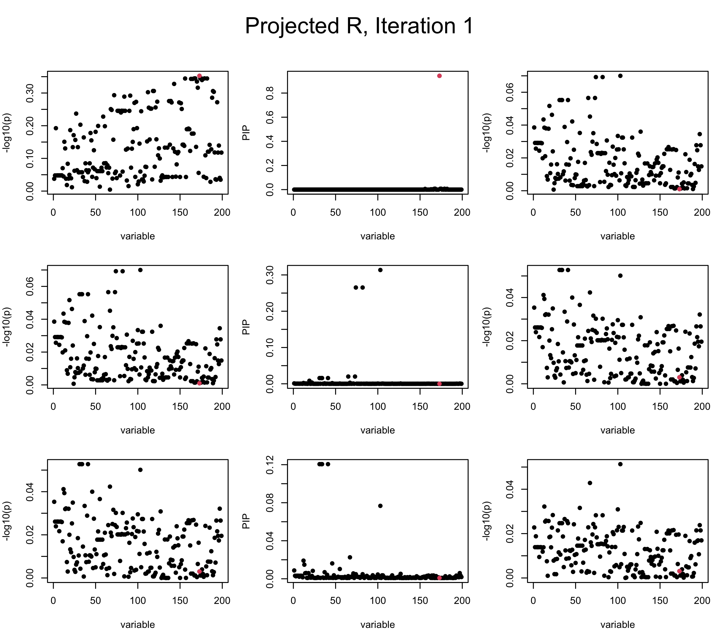
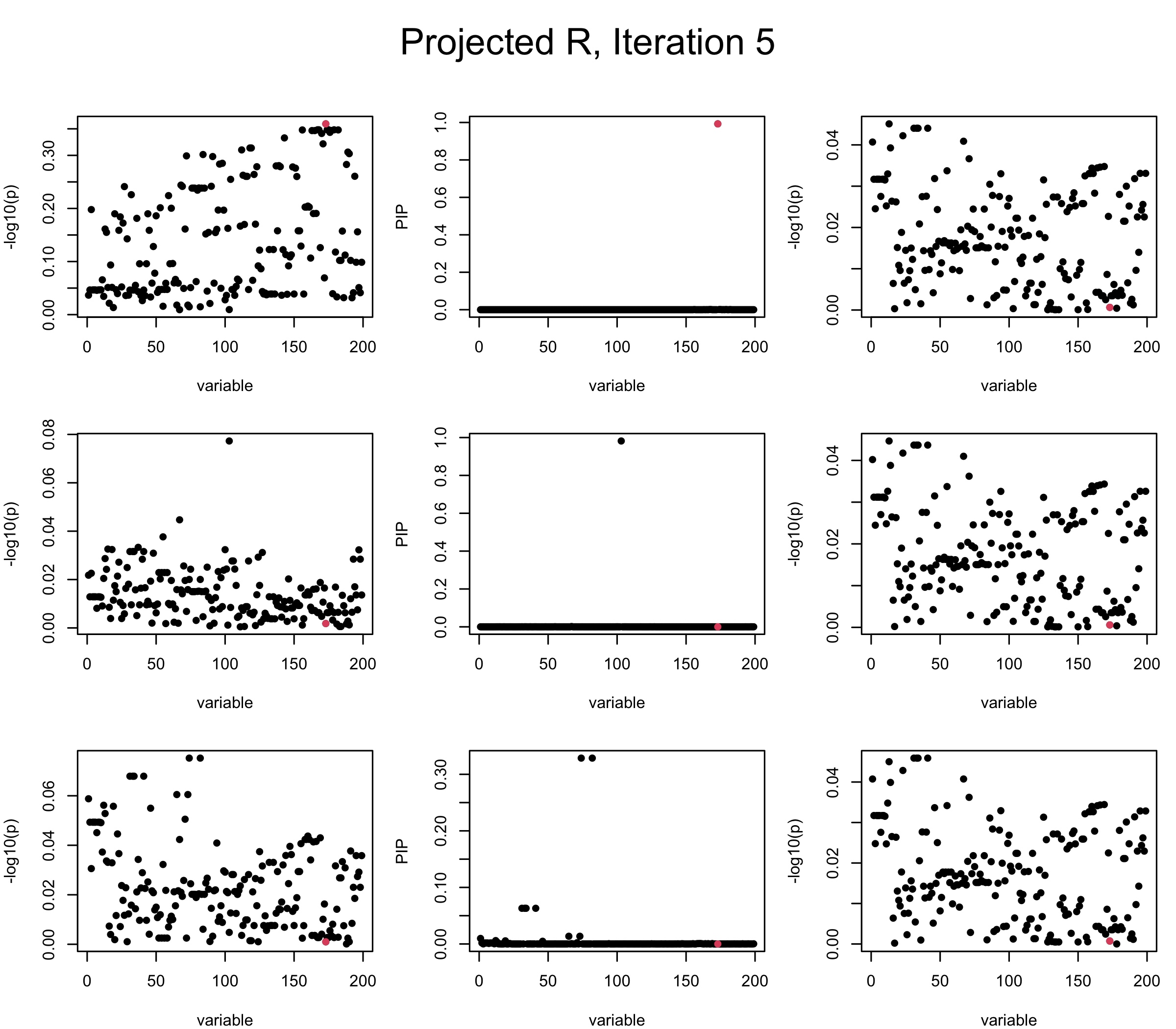
In the experiment below, the true \(L = 1\) and causal SNP’s position is randomly chosen between 1 and \(J = 200\). Set \(L = 3\) in SuSiE and in every iteration, we will look at three figures: (1) \(\overline{r}\) after adding back \(\ell\)-th CS; (2) PIP got from Single Effect Model; (3) \(\overline{r}\) after subtracting \(R \overline{b}\). We consider In-sample, Out-of-sample, and Projected (our method) covariance matrices.
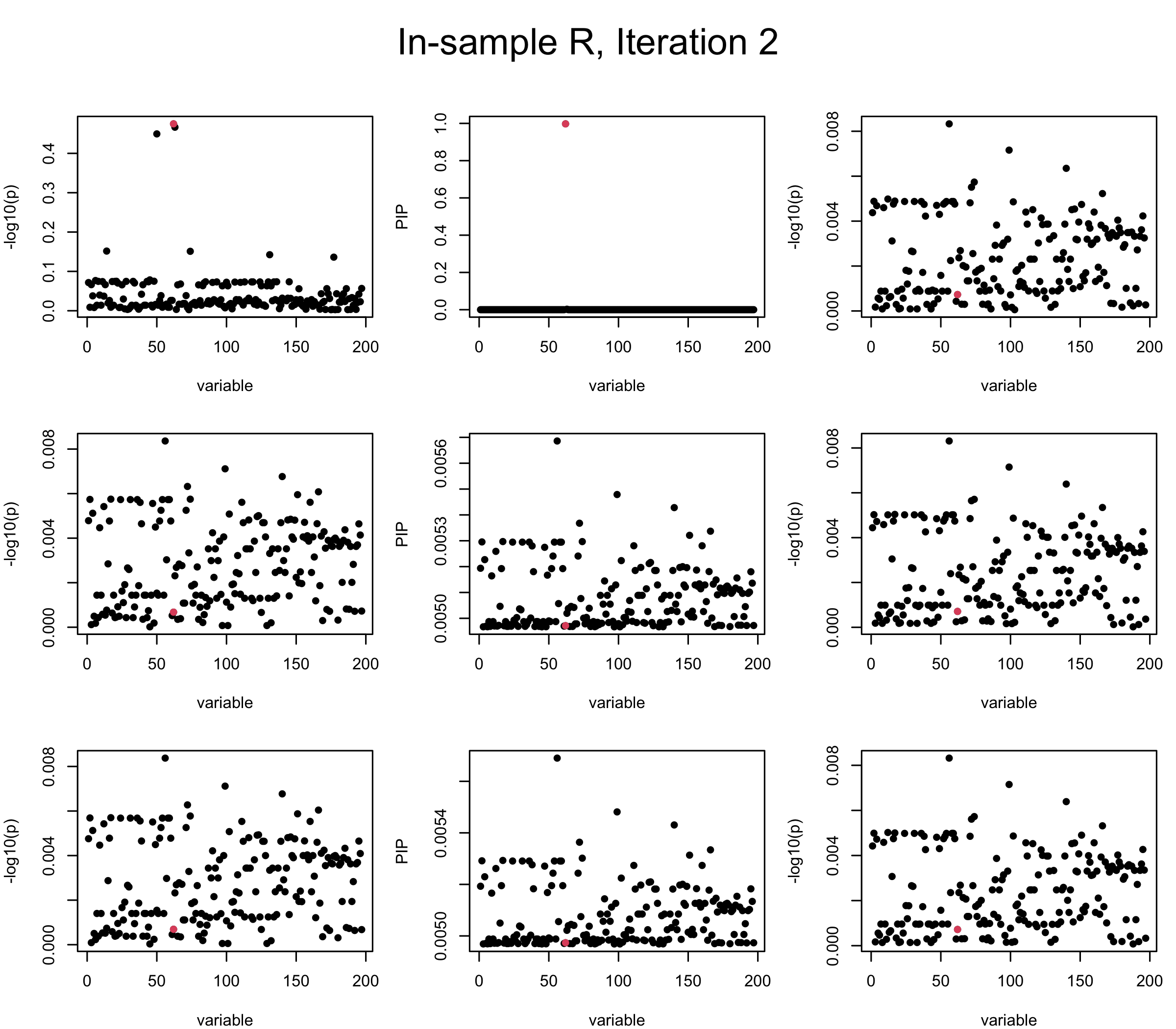
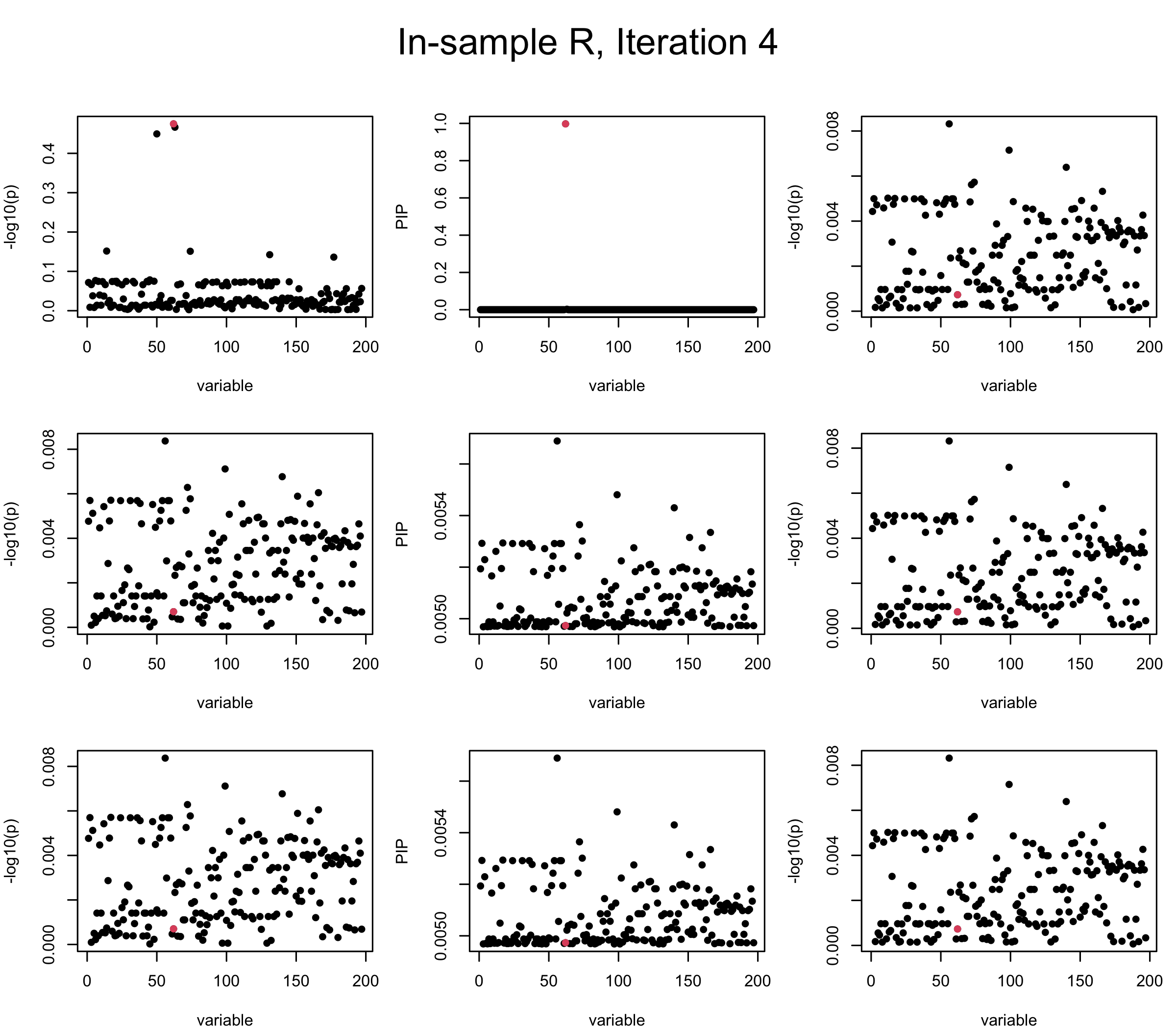
Note that the title of the figure corresponds to SuSiE’s outer loop. Each figure has 3 rows correspond to the inner loop from 1 to \(L = 3\). The algorithm often converges after around 5 iteration (outer loop) so we only look at the first 5.
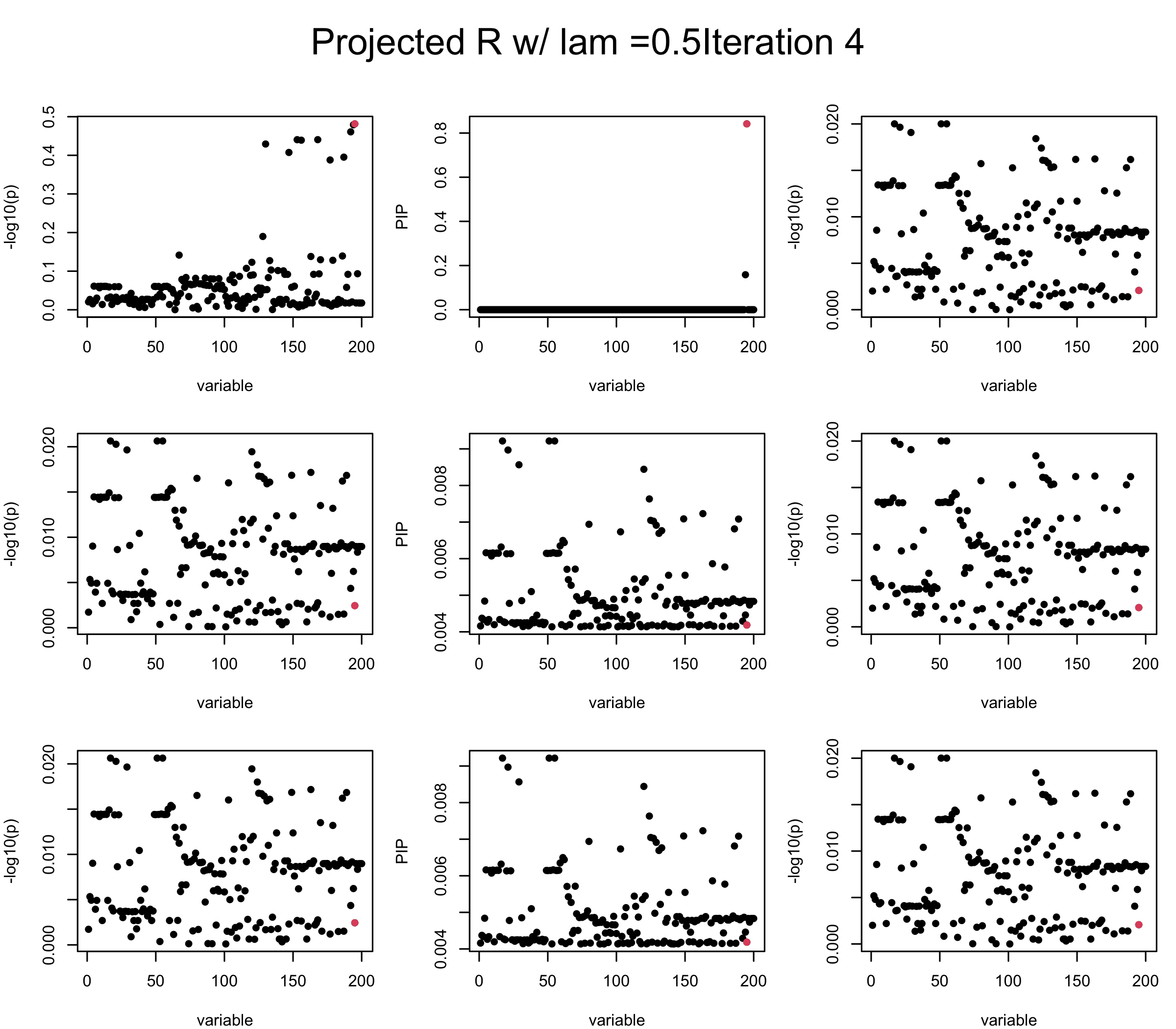
It is helpful to pay attention to the scale of \(y\)-axis (of \(v\) and of PIP) in each figure, as it can change from figure to figure.
First we look at In-sample Covariance matrix. All is good
knitr::opts_chunk$set(echo = TRUE, fig.width=8, fig.height=7, dpi=150)
library(susieR)
source("code/SuSiE_rss.R")
source("code/R_algorithms.R")

## using gtex data
gtex = readRDS("./data/Thyroid_ENSG00000132855.rds")

## seed present: 1, 2
seed = 1
set.seed(seed)
print(paste("This is seed number", seed))
[1] "This is seed number 1"# Remove SNPs with MAF < 0.01
maf = apply(gtex, 2, function(x) sum(x)/2/length(x))
X0 = gtex[, maf > 0.01]
X = na.omit(X0)
snp_total = ncol(X0)
n = nrow(X0)
J = 200
# Start from a random point on the genome
indx_start = sample(1: (snp_total - J), 1)
X = X0[, indx_start:(indx_start + J -1)]
# View(cor(X)[1:10, 1:10])
## sub-sample into two
out_sample = sample(1:n, 100)
X_out = X[out_sample, ]
X_in = X[setdiff(1:n, out_sample), ]
rm_p = c(which(diag(cov(X_in))==0), which(diag(cov(X_out))==0))
indx_p = setdiff(1:J, rm_p)
X_in = X_in[, indx_p]
X_out = X_out[, indx_p]
## Standardize both sample matrices
X_in <- scale(X_in)
X_out <- scale(X_out)
## out-sample LD matrix
R_hat = cor(X_out)
R = cor(X_in)
## generate data from in-sample X matrix
J = ncol(X_in)
beta <- rep(0, J)
n = nrow(X_in)
num_causal_SNP = 1
gamma = sample(c(1:J), size = num_causal_SNP, replace = FALSE)
b = rnorm(num_causal_SNP) * 3
beta = rep(0, J)
beta[gamma] = b
y = X_in %*% beta + rnorm(n)
y = scale(y)
V_xy = t(X_in) %*% y / (n-1)
## 1. In-sample covariance matrix
V_xx = R
sigma2 = 1
sigma02 = 1
L = 3
max_iter = 5
b_bar = matrix(0, nrow = L, ncol = J)
b_bar2 = matrix(0, nrow = L, ncol = J)
alphas = matrix(0, nrow = L, ncol = J)
mus = matrix(0, nrow = L, ncol = J)
sigmas = matrix(0, nrow = L, ncol = J)
for (iter in (1:max_iter)){
par(mfrow = c(3, 3), mar = c(4, 4, 2, 1), oma = c(0, 0, 4, 0))
V_xy_bar = V_xy - V_xx %*% colSums(b_bar) ## residual signal
for (ell in 1:L){
V_xy_bar_ell = V_xy_bar + V_xx %*% b_bar[ell, ] ## add back ell-th signal
susie_plot(V_xy_bar_ell, y = "z", b=beta)
ret = SER(V_xx, V_xy_bar_ell, n, sigma2, sigma02)
alphas[ell, ] = ret$alpha
mus[ell, ] = ret$mus
sigmas[ell, ] = ret$sigma12
b_bar[ell, ] = alphas[ell, ] * mus[ell, ]
b_bar2[ell, ] = alphas[ell, ] * (mus[ell, ]^2 + sigmas[ell, ])
V_xy_bar = V_xy_bar_ell - V_xx %*% b_bar[ell, ]
susie_plot(ret$alpha, y = "PIP", b=beta)
susie_plot(V_xy_bar, y = "z", b=beta)
}
mtext(paste0("In-sample R, Iteration ", iter), outer = TRUE, cex = 1.5, line = 1)
}


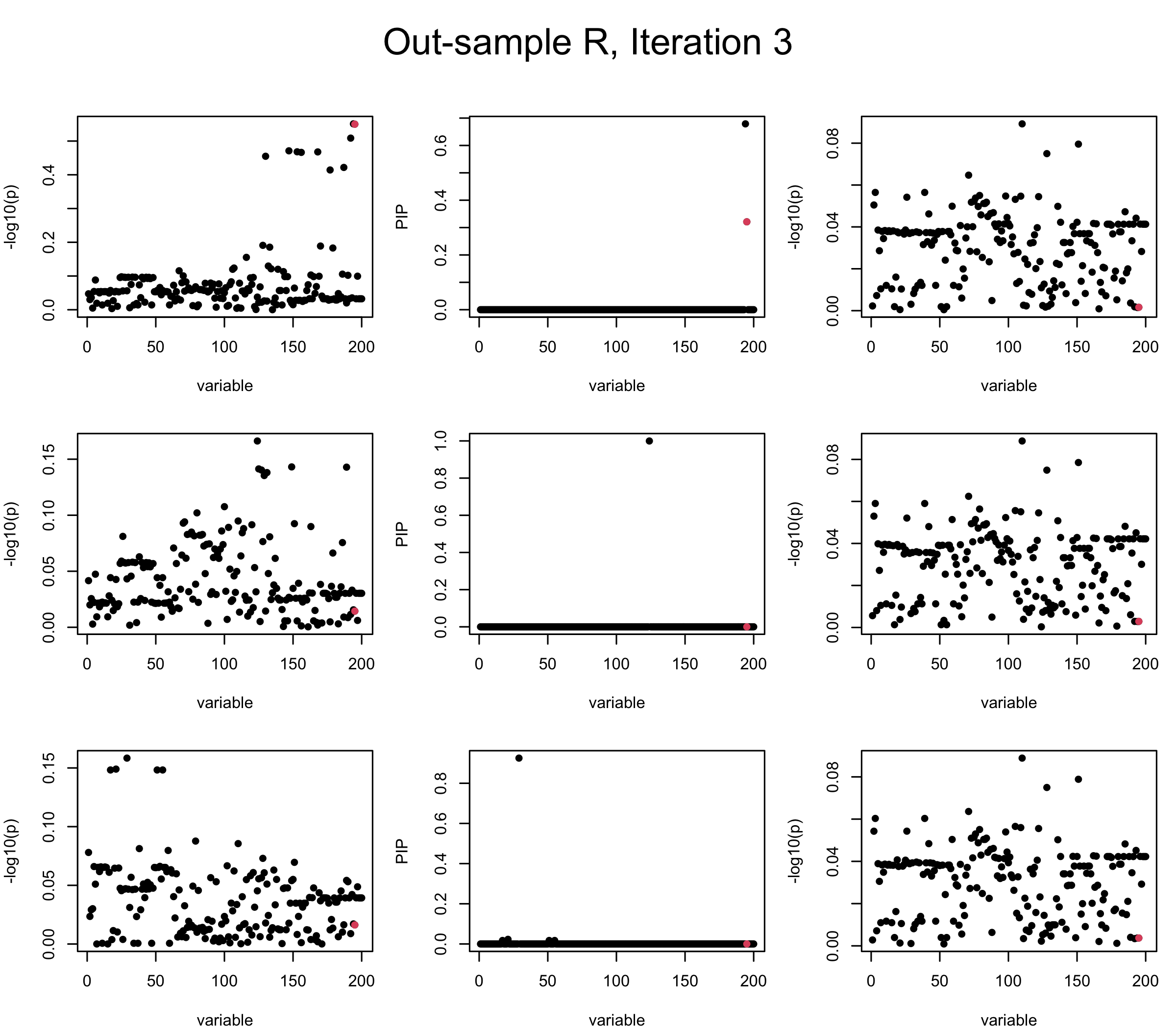
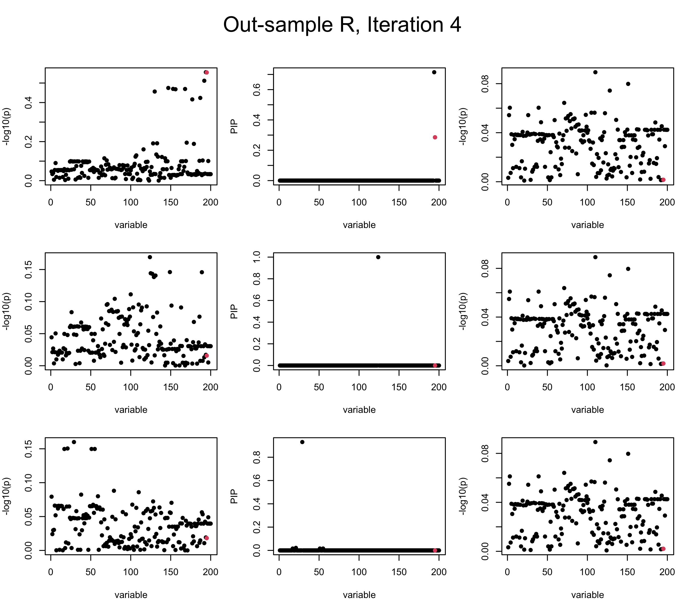
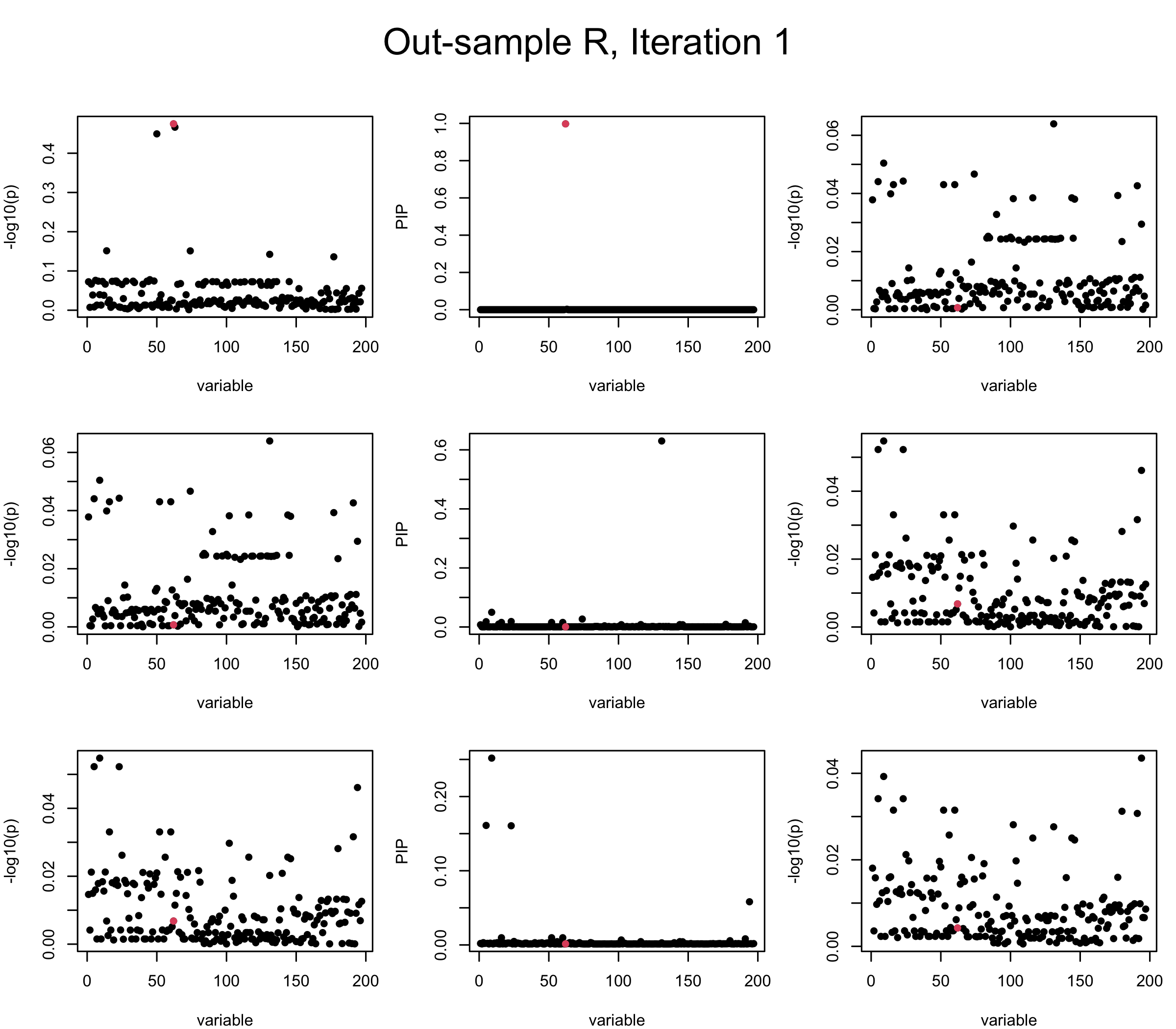
Out-sample Covariance matrix: We can see that after subtracting the first CS, the remaining \(\overline{v}\) is still big (not subtracting enough; compare to the in-sample covariance matrix).
## 2. Out-sample covariance matrix
V_xx = R_hat
sigma2 = 1
sigma02 = 1
L = 3
 max_iter = 5

b_bar = matrix(0, nrow = L, ncol = J)
b_bar2 = matrix(0, nrow = L, ncol = J)
alphas = matrix(0, nrow = L, ncol = J)
mus = matrix(0, nrow = L, ncol = J)
sigmas = matrix(0, nrow = L, ncol = J)


for (iter in (1:max_iter)){
  par(mfrow = c(3, 3), mar = c(4, 4, 2, 1), oma = c(0, 0, 4, 0))
  V_xy_bar = V_xy - V_xx %*% colSums(b_bar)  ## residual signal

  for (ell in 1:L){
    V_xy_bar_ell = V_xy_bar + V_xx %*% b_bar[ell, ]  ## add back ell-th signal

    susie_plot(V_xy_bar_ell, y = "z", b=beta)

    ret = SER(V_xx, V_xy_bar_ell, n, sigma2, sigma02)
    alphas[ell, ] = ret$alpha
    mus[ell, ] = ret$mus
    sigmas[ell, ] = ret$sigma12
    b_bar[ell, ] = alphas[ell, ] * mus[ell, ]
    b_bar2[ell, ] = alphas[ell, ] * (mus[ell, ]^2 + sigmas[ell, ])
    V_xy_bar = V_xy_bar_ell - V_xx %*% b_bar[ell, ]

    susie_plot(ret$alpha, y = "PIP", b=beta)
    susie_plot(V_xy_bar, y = "z", b=beta)

  }
  mtext(paste0("Out-sample R, Iteration ", iter), outer = TRUE, cex = 1.5, line = 1)
}


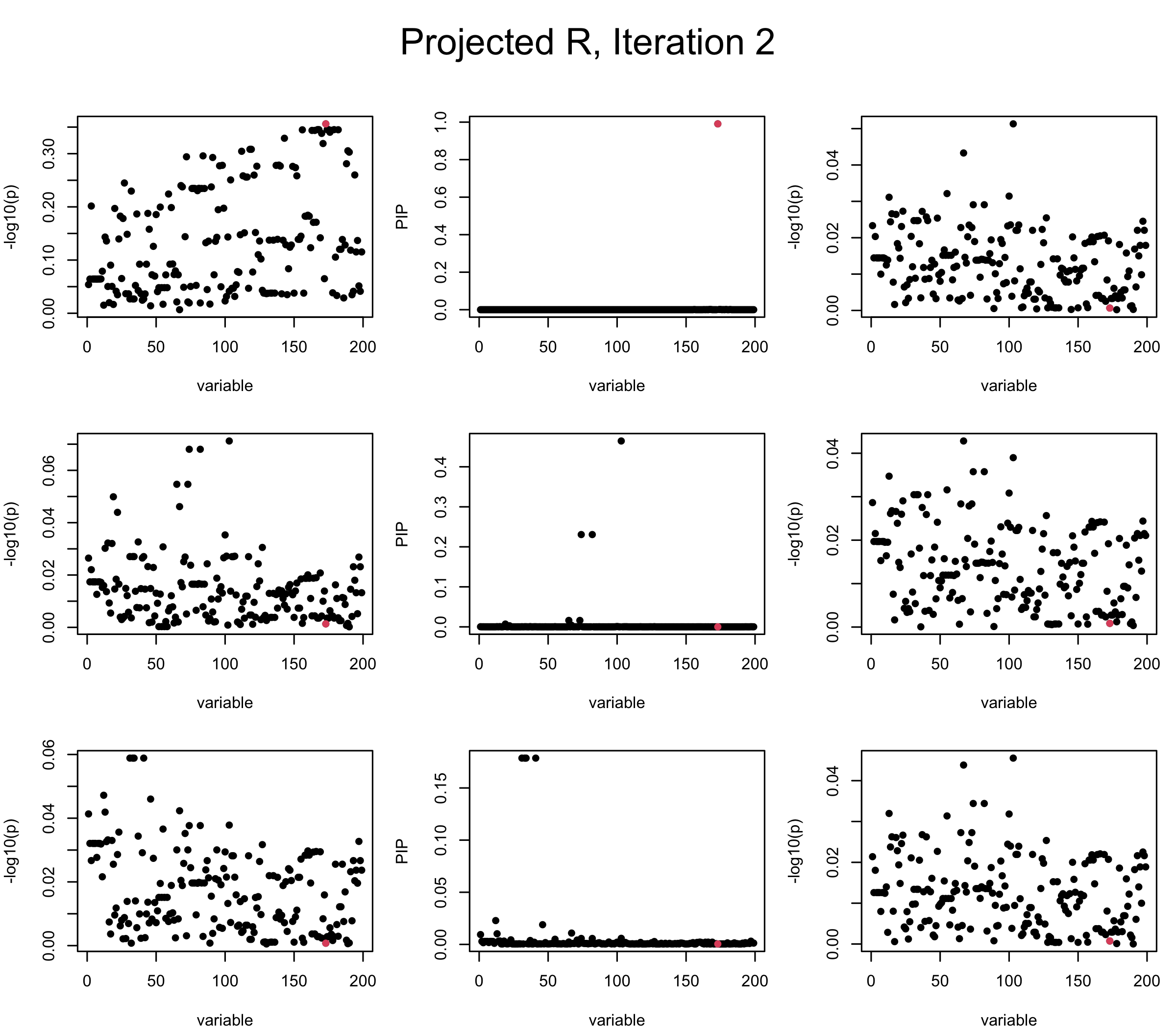
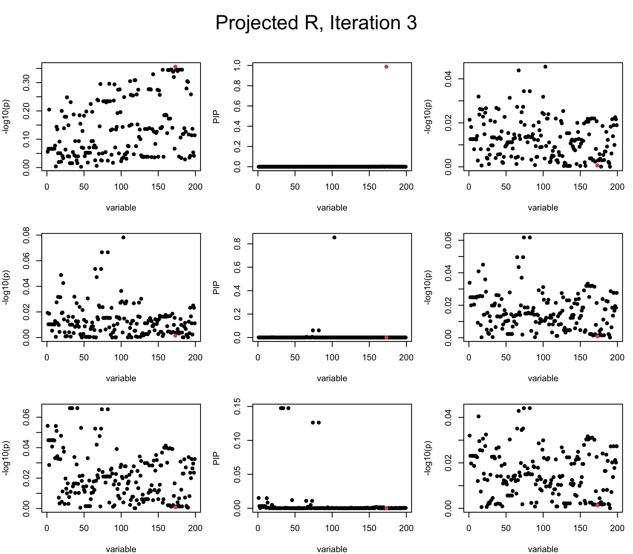
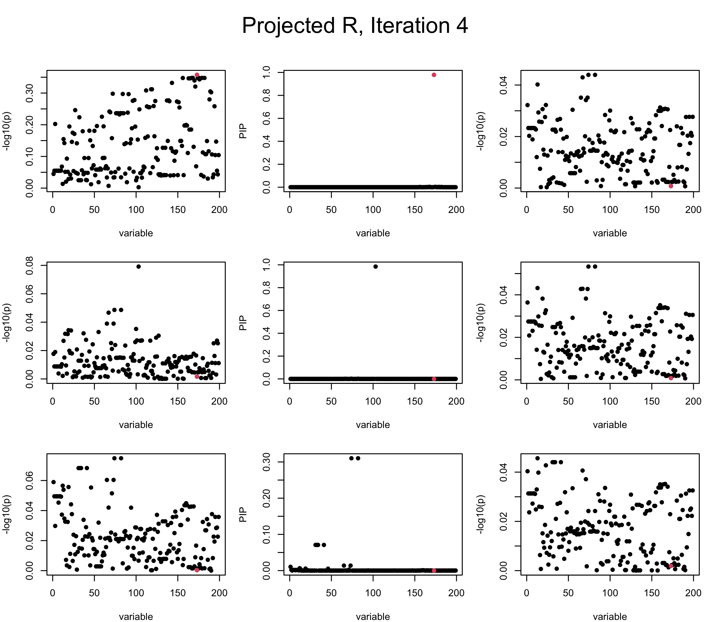
Projected Covariance matrix: After subtracting the first CS, the remaining \(\overline{v}\) is better controlled.
## 3. Projected R
ret = proj_Dykstra(R=R_hat, v=V_xy)
V_xx = ret$R
sigma2 = 1
sigma02 = 1
L = 3
 max_iter = 5

b_bar = matrix(0, nrow = L, ncol = J)
b_bar2 = matrix(0, nrow = L, ncol = J)
alphas = matrix(0, nrow = L, ncol = J)
mus = matrix(0, nrow = L, ncol = J)
sigmas = matrix(0, nrow = L, ncol = J)


for (iter in (1:max_iter)){
  par(mfrow = c(3, 3), mar = c(4, 4, 2, 1), oma = c(0, 0, 4, 0))
  V_xy_bar = V_xy - V_xx %*% colSums(b_bar)  ## residual signal

  for (ell in 1:L){
    V_xy_bar_ell = V_xy_bar + V_xx %*% b_bar[ell, ]  ## add back ell-th signal

    susie_plot(V_xy_bar_ell, y = "z", b=beta)

    ret = SER(V_xx, V_xy_bar_ell, n, sigma2, sigma02)
    alphas[ell, ] = ret$alpha
    mus[ell, ] = ret$mus
    sigmas[ell, ] = ret$sigma12
    b_bar[ell, ] = alphas[ell, ] * mus[ell, ]
    b_bar2[ell, ] = alphas[ell, ] * (mus[ell, ]^2 + sigmas[ell, ])
    V_xy_bar = V_xy_bar_ell - V_xx %*% b_bar[ell, ]

    susie_plot(ret$alpha, y = "PIP", b=beta)
    susie_plot(V_xy_bar, y = "z", b=beta)

  }
  mtext(paste0("Projected R, Iteration ", iter), outer = TRUE, cex = 1.5, line = 1)
}


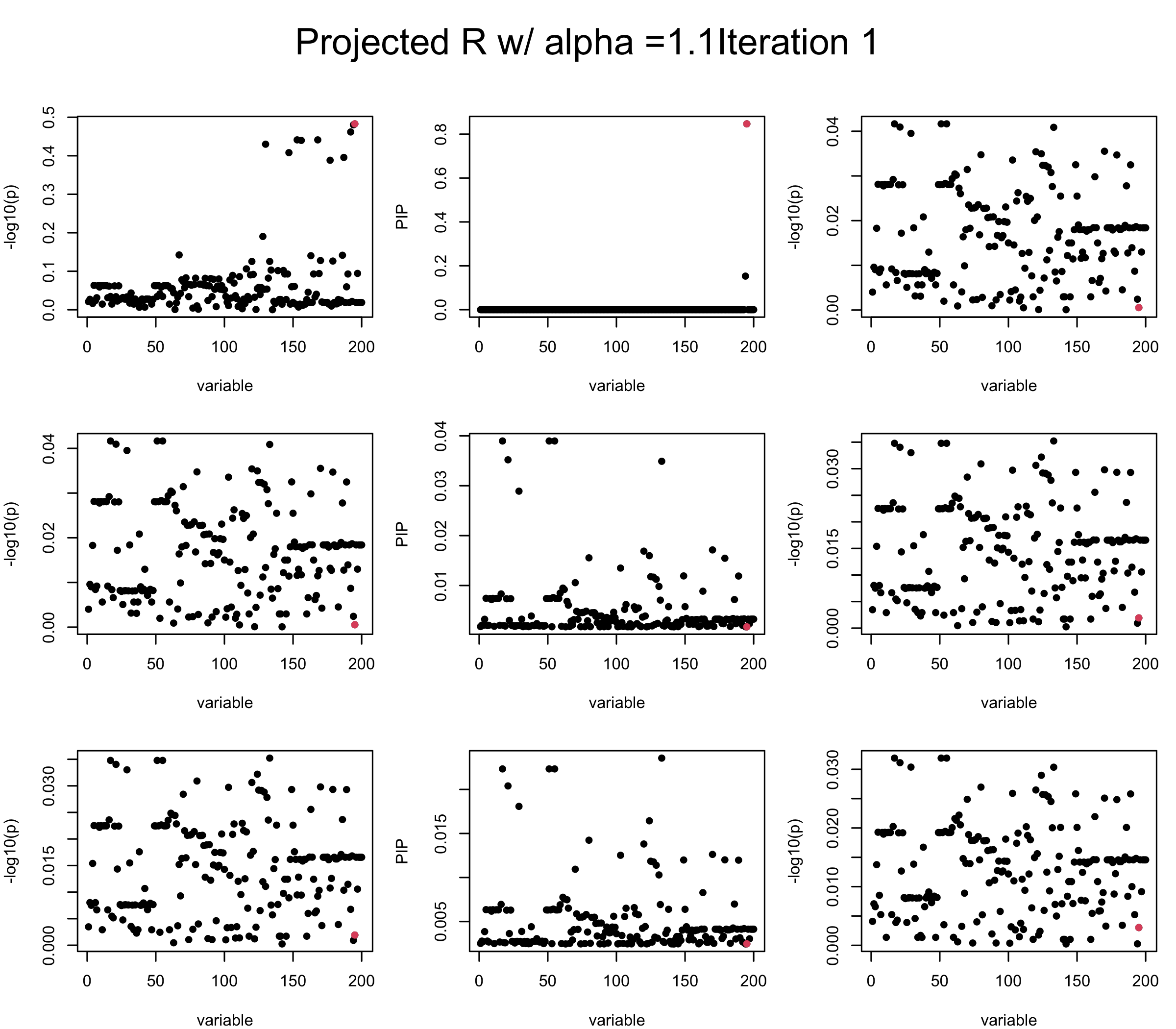
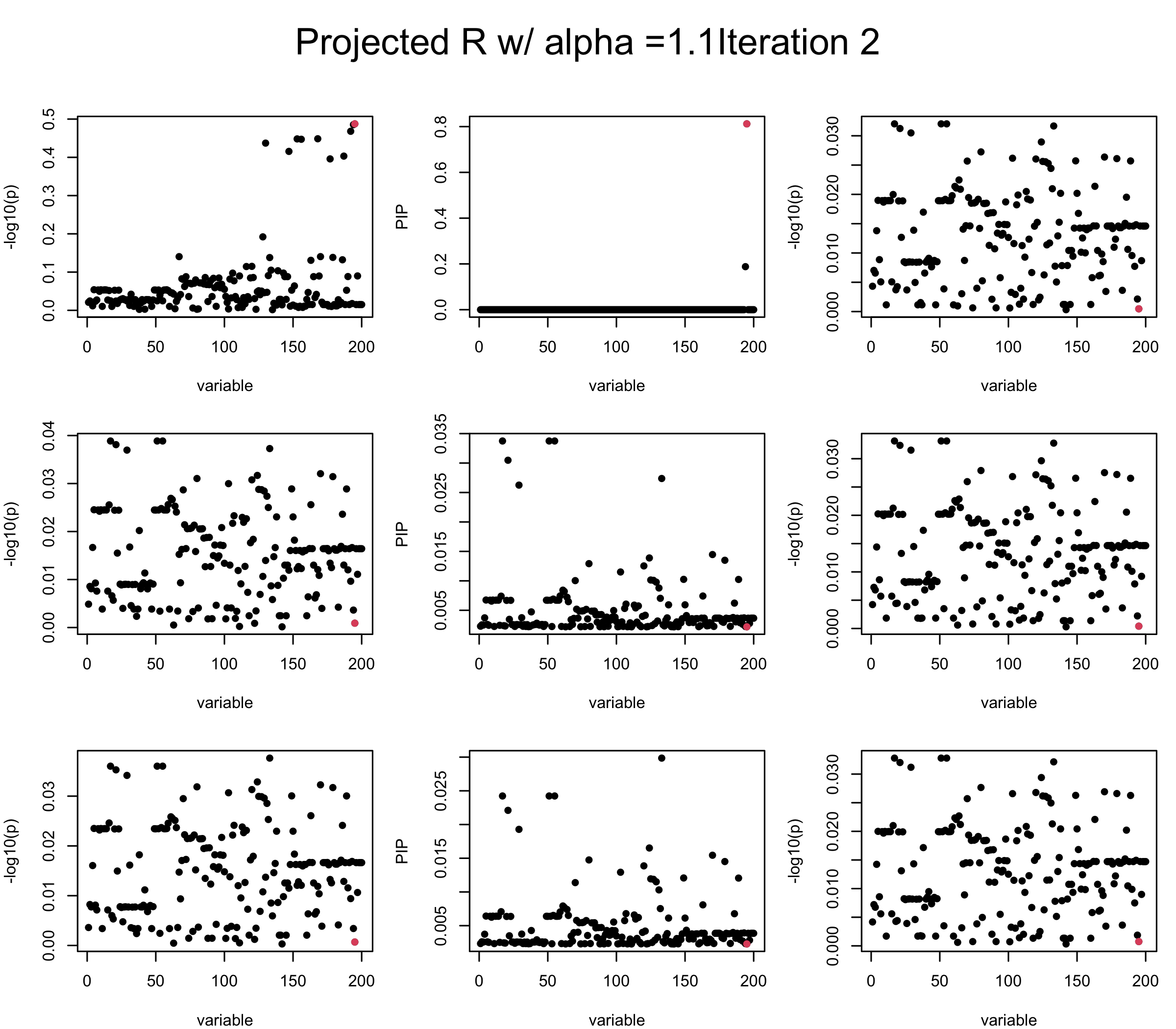
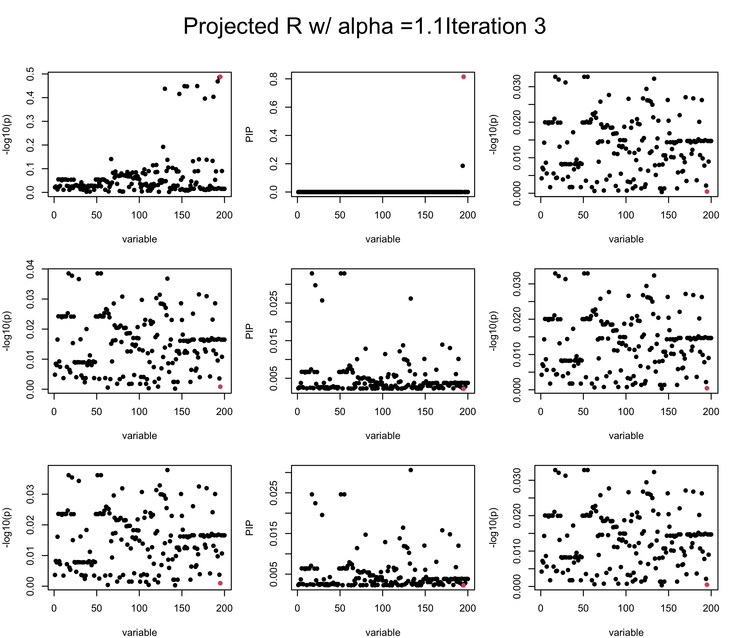
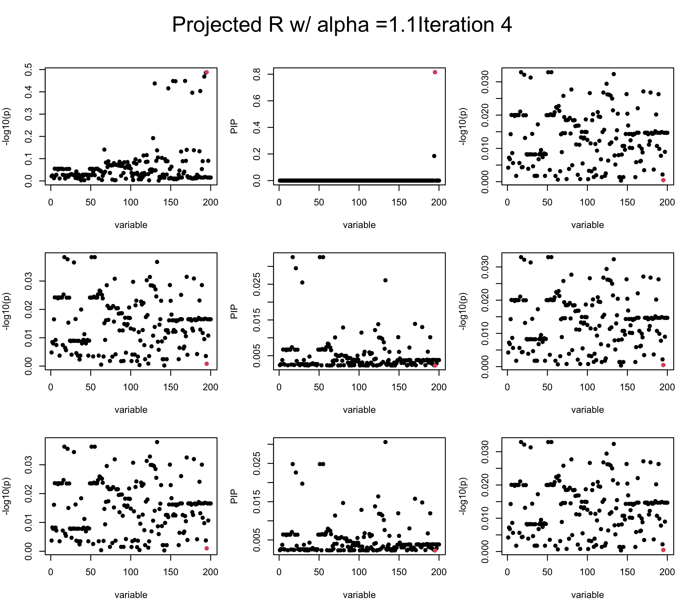
Consider multiplying \(vv^{\top}\) with some \(\alpha > 1\). We find that it does not improve control of the residual. When setting \(\alpha > 1.4\), SuSiE often gives error in training….
alpha = 1.1
ret = proj_Dykstra(R=R_hat, v= sqrt(alpha) * V_xy)
sigma2 = 1
sigma02 = 1
L = 3
max_iter = 5

b_bar = matrix(0, nrow = L, ncol = J)
b_bar2 = matrix(0, nrow = L, ncol = J)
alphas = matrix(0, nrow = L, ncol = J)
mus = matrix(0, nrow = L, ncol = J)
sigmas = matrix(0, nrow = L, ncol = J)


for (iter in (1:max_iter)){
  par(mfrow = c(3, 3), mar = c(4, 4, 2, 1), oma = c(0, 0, 4, 0))
  V_xy_bar = V_xy - V_xx %*% colSums(b_bar)  ## residual signal

  for (ell in 1:L){
    V_xy_bar_ell = V_xy_bar + V_xx %*% b_bar[ell, ]  ## add back ell-th signal

    susie_plot(V_xy_bar_ell, y = "z", b=beta)

    ret = SER(V_xx, V_xy_bar_ell, n, sigma2, sigma02)
    alphas[ell, ] = ret$alpha
    mus[ell, ] = ret$mus
    sigmas[ell, ] = ret$sigma12
    b_bar[ell, ] = alphas[ell, ] * mus[ell, ]
    b_bar2[ell, ] = alphas[ell, ] * (mus[ell, ]^2 + sigmas[ell, ])
    V_xy_bar = V_xy_bar_ell - V_xx %*% b_bar[ell, ]

    susie_plot(ret$alpha, y = "PIP", b=beta)
    susie_plot(V_xy_bar, y = "z", b=beta)

  }
  mtext(paste0("Projected R w/ alpha =", alpha, "Iteration ", iter), outer = TRUE, cex = 1.5, line = 1)
}

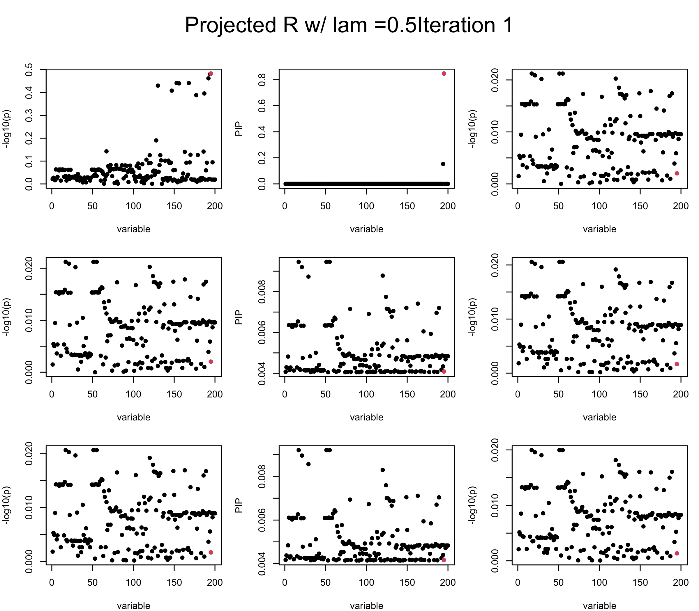
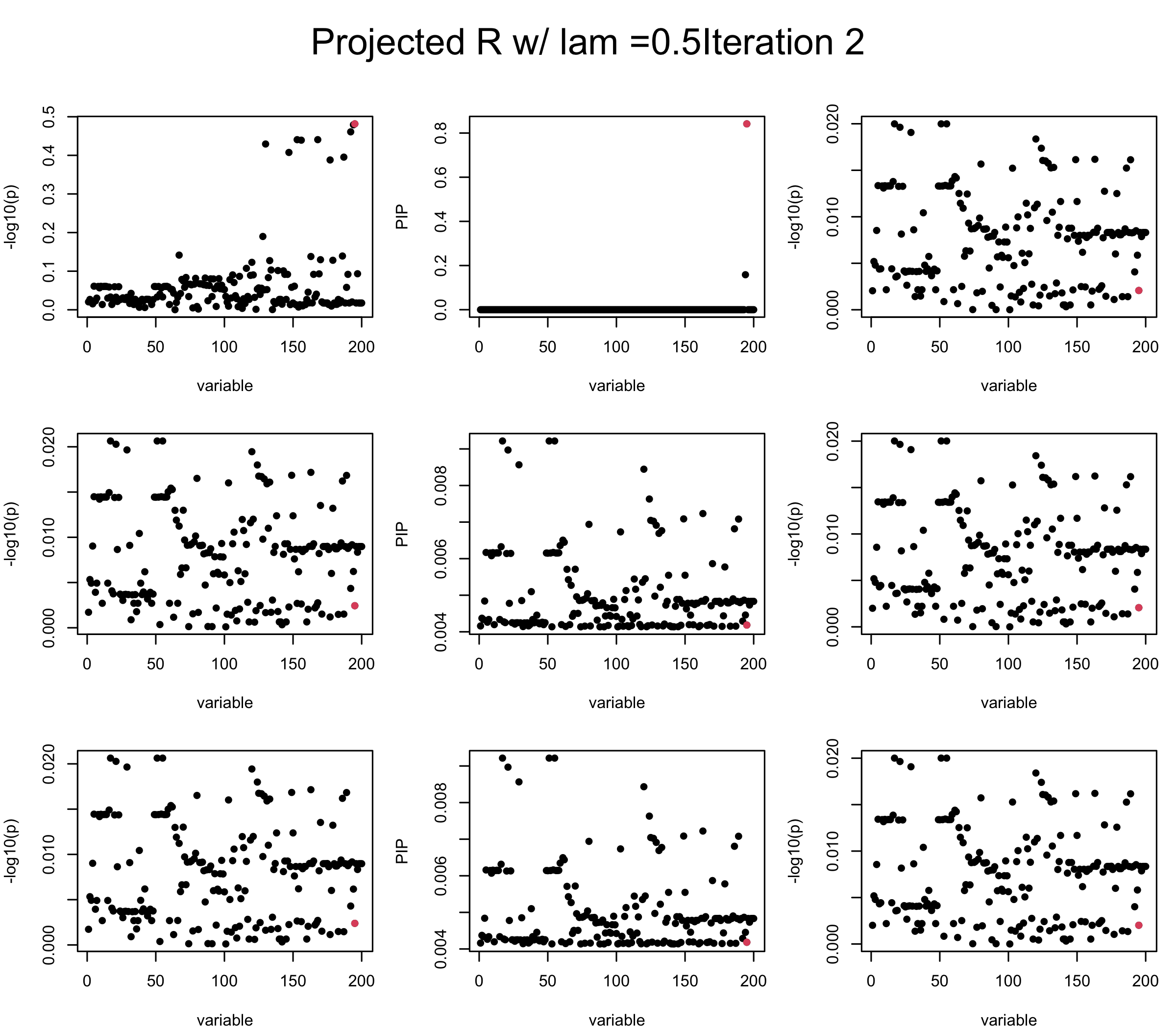
Let us experiment with interpolating between Projected \(\tilde{R}\) and \(vv^{\top}\) Consider \(R = \lambda \tilde{R} + (1-\lambda) vv^{\top}\) and set \(diag(R) = 1\). We find it helps controlling the residual a little bit.
lam = 0.5
ret = proj_Dykstra(R=R_hat, v = V_xy)
V_xx = lam * ret$R + (1-lam) * tcrossprod(V_xy)
diag(V_xx) <- 1
sigma2 = 1
sigma02 = 1
L = 3
 max_iter = 5

b_bar = matrix(0, nrow = L, ncol = J)
b_bar2 = matrix(0, nrow = L, ncol = J)
alphas = matrix(0, nrow = L, ncol = J)
mus = matrix(0, nrow = L, ncol = J)
sigmas = matrix(0, nrow = L, ncol = J)


for (iter in (1:max_iter)){
  par(mfrow = c(3, 3), mar = c(4, 4, 2, 1), oma = c(0, 0, 4, 0))
  V_xy_bar = V_xy - V_xx %*% colSums(b_bar)  ## residual signal

  for (ell in 1:L){
    V_xy_bar_ell = V_xy_bar + V_xx %*% b_bar[ell, ]  ## add back ell-th signal

    susie_plot(V_xy_bar_ell, y = "z", b=beta)

    ret = SER(V_xx, V_xy_bar_ell, n, sigma2, sigma02)
    alphas[ell, ] = ret$alpha
    mus[ell, ] = ret$mus
    sigmas[ell, ] = ret$sigma12
    b_bar[ell, ] = alphas[ell, ] * mus[ell, ]
    b_bar2[ell, ] = alphas[ell, ] * (mus[ell, ]^2 + sigmas[ell, ])
    V_xy_bar = V_xy_bar_ell - V_xx %*% b_bar[ell, ]

    susie_plot(ret$alpha, y = "PIP", b=beta)
    susie_plot(V_xy_bar, y = "z", b=beta)

  }
  mtext(paste0("Projected R w/ lam =", lam, "Iteration ", iter), outer = TRUE, cex = 1.5, line = 1)
}


Let us look at some other seeds.
seed = 1
set.seed(seed)
print(paste("This is seed number", seed))
[1] "This is seed number 1"# Remove SNPs with MAF < 0.01
maf = apply(gtex, 2, function(x) sum(x)/2/length(x))
X0 = gtex[, maf > 0.01]
X = na.omit(X0)
snp_total = ncol(X0)
n = nrow(X0)
J = 200
# Start from a random point on the genome
indx_start = sample(1: (snp_total - J), 1)
X = X0[, indx_start:(indx_start + J -1)]
# View(cor(X)[1:10, 1:10])
## sub-sample into two
out_sample = sample(1:n, 100)
X_out = X[out_sample, ]
X_in = X[setdiff(1:n, out_sample), ]
rm_p = c(which(diag(cov(X_in))==0), which(diag(cov(X_out))==0))
indx_p = setdiff(1:J, rm_p)
X_in = X_in[, indx_p]
X_out = X_out[, indx_p]
## Standardize both sample matrices
X_in <- scale(X_in)
X_out <- scale(X_out)
## out-sample LD matrix
R_hat = cor(X_out)
R = cor(X_in)
## generate data from in-sample X matrix
J = ncol(X_in)
beta <- rep(0, J)
n = nrow(X_in)
num_causal_SNP = 1
gamma = sample(c(1:J), size = num_causal_SNP, replace = FALSE)
b = rnorm(num_causal_SNP) * 3
beta = rep(0, J)
beta[gamma] = b
y = X_in %*% beta + rnorm(n)
y = scale(y)
V_xy = t(X_in) %*% y / (n-1)
## 1. In-sample covariance matrix
V_xx = R
sigma2 = 1
sigma02 = 1
L = 3
max_iter = 5
b_bar = matrix(0, nrow = L, ncol = J)
b_bar2 = matrix(0, nrow = L, ncol = J)
alphas = matrix(0, nrow = L, ncol = J)
mus = matrix(0, nrow = L, ncol = J)
sigmas = matrix(0, nrow = L, ncol = J)
for (iter in (1:max_iter)){
par(mfrow = c(3, 3), mar = c(4, 4, 2, 1), oma = c(0, 0, 4, 0))
V_xy_bar = V_xy - V_xx %*% colSums(b_bar) ## residual signal
for (ell in 1:L){
V_xy_bar_ell = V_xy_bar + V_xx %*% b_bar[ell, ] ## add back ell-th signal
susie_plot(V_xy_bar_ell, y = "z", b=beta)
ret = SER(V_xx, V_xy_bar_ell, n, sigma2, sigma02)
alphas[ell, ] = ret$alpha
mus[ell, ] = ret$mus
sigmas[ell, ] = ret$sigma12
b_bar[ell, ] = alphas[ell, ] * mus[ell, ]
b_bar2[ell, ] = alphas[ell, ] * (mus[ell, ]^2 + sigmas[ell, ])
V_xy_bar = V_xy_bar_ell - V_xx %*% b_bar[ell, ]
susie_plot(ret$alpha, y = "PIP", b=beta)
susie_plot(V_xy_bar, y = "z", b=beta)
}
mtext(paste0("In-sample R, Iteration ", iter), outer = TRUE, cex = 1.5, line = 1)
}


## 2. Out-sample covariance matrix
V_xx = R_hat
sigma2 = 1
sigma02 = 1
L = 3
 max_iter = 5

b_bar = matrix(0, nrow = L, ncol = J)
b_bar2 = matrix(0, nrow = L, ncol = J)
alphas = matrix(0, nrow = L, ncol = J)
mus = matrix(0, nrow = L, ncol = J)
sigmas = matrix(0, nrow = L, ncol = J)


for (iter in (1:max_iter)){
  par(mfrow = c(3, 3), mar = c(4, 4, 2, 1), oma = c(0, 0, 4, 0))
  V_xy_bar = V_xy - V_xx %*% colSums(b_bar)  ## residual signal

  for (ell in 1:L){
    V_xy_bar_ell = V_xy_bar + V_xx %*% b_bar[ell, ]  ## add back ell-th signal

    susie_plot(V_xy_bar_ell, y = "z", b=beta)

    ret = SER(V_xx, V_xy_bar_ell, n, sigma2, sigma02)
    alphas[ell, ] = ret$alpha
    mus[ell, ] = ret$mus
    sigmas[ell, ] = ret$sigma12
    b_bar[ell, ] = alphas[ell, ] * mus[ell, ]
    b_bar2[ell, ] = alphas[ell, ] * (mus[ell, ]^2 + sigmas[ell, ])
    V_xy_bar = V_xy_bar_ell - V_xx %*% b_bar[ell, ]

    susie_plot(ret$alpha, y = "PIP", b=beta)
    susie_plot(V_xy_bar, y = "z", b=beta)

  }
  mtext(paste0("Out-sample R, Iteration ", iter), outer = TRUE, cex = 1.5, line = 1)
}


## 3. Projected R
ret = proj_Dykstra(R=R_hat, v=V_xy)
V_xx = ret$R
sigma2 = 1
sigma02 = 1
L = 3
 max_iter = 5

b_bar = matrix(0, nrow = L, ncol = J)
b_bar2 = matrix(0, nrow = L, ncol = J)
alphas = matrix(0, nrow = L, ncol = J)
mus = matrix(0, nrow = L, ncol = J)
sigmas = matrix(0, nrow = L, ncol = J)


for (iter in (1:max_iter)){
  par(mfrow = c(3, 3), mar = c(4, 4, 2, 1), oma = c(0, 0, 4, 0))
  V_xy_bar = V_xy - V_xx %*% colSums(b_bar)  ## residual signal

  for (ell in 1:L){
    V_xy_bar_ell = V_xy_bar + V_xx %*% b_bar[ell, ]  ## add back ell-th signal

    susie_plot(V_xy_bar_ell, y = "z", b=beta)

    ret = SER(V_xx, V_xy_bar_ell, n, sigma2, sigma02)
    alphas[ell, ] = ret$alpha
    mus[ell, ] = ret$mus
    sigmas[ell, ] = ret$sigma12
    b_bar[ell, ] = alphas[ell, ] * mus[ell, ]
    b_bar2[ell, ] = alphas[ell, ] * (mus[ell, ]^2 + sigmas[ell, ])
    V_xy_bar = V_xy_bar_ell - V_xx %*% b_bar[ell, ]

    susie_plot(ret$alpha, y = "PIP", b=beta)
    susie_plot(V_xy_bar, y = "z", b=beta)

  }
  mtext(paste0("Projected R, Iteration ", iter), outer = TRUE, cex = 1.5, line = 1)
}
| Version | Author | Date |
|---|---|---|
| 2f35f45 | dodat97 | 2025-09-09 |
| Version | Author | Date |
|---|---|---|
| 2f35f45 | dodat97 | 2025-09-09 |

| Version | Author | Date |
|---|---|---|
| 2f35f45 | dodat97 | 2025-09-09 |

| Version | Author | Date |
|---|---|---|
| 2f35f45 | dodat97 | 2025-09-09 |

| Version | Author | Date |
|---|---|---|
| 2f35f45 | dodat97 | 2025-09-09 |
seed = 2
set.seed(seed)
print(paste("This is seed number", seed))
[1] "This is seed number 2"# Remove SNPs with MAF < 0.01
maf = apply(gtex, 2, function(x) sum(x)/2/length(x))
X0 = gtex[, maf > 0.01]
X = na.omit(X0)
snp_total = ncol(X0)
n = nrow(X0)
J = 200
# Start from a random point on the genome
indx_start = sample(1: (snp_total - J), 1)
X = X0[, indx_start:(indx_start + J -1)]
# View(cor(X)[1:10, 1:10])
## sub-sample into two
out_sample = sample(1:n, 100)
X_out = X[out_sample, ]
X_in = X[setdiff(1:n, out_sample), ]
rm_p = c(which(diag(cov(X_in))==0), which(diag(cov(X_out))==0))
indx_p = setdiff(1:J, rm_p)
X_in = X_in[, indx_p]
X_out = X_out[, indx_p]
## Standardize both sample matrices
X_in <- scale(X_in)
X_out <- scale(X_out)
## out-sample LD matrix
R_hat = cor(X_out)
R = cor(X_in)
## generate data from in-sample X matrix
J = ncol(X_in)
beta <- rep(0, J)
n = nrow(X_in)
num_causal_SNP = 1
gamma = sample(c(1:J), size = num_causal_SNP, replace = FALSE)
b = rnorm(num_causal_SNP) * 3
beta = rep(0, J)
beta[gamma] = b
y = X_in %*% beta + rnorm(n)
y = scale(y)
V_xy = t(X_in) %*% y / (n-1)
## 1. In-sample covariance matrix
V_xx = R
sigma2 = 1
sigma02 = 1
L = 3
max_iter = 5
b_bar = matrix(0, nrow = L, ncol = J)
b_bar2 = matrix(0, nrow = L, ncol = J)
alphas = matrix(0, nrow = L, ncol = J)
mus = matrix(0, nrow = L, ncol = J)
sigmas = matrix(0, nrow = L, ncol = J)
for (iter in (1:max_iter)){
par(mfrow = c(3, 3), mar = c(4, 4, 2, 1), oma = c(0, 0, 4, 0))
V_xy_bar = V_xy - V_xx %*% colSums(b_bar) ## residual signal
for (ell in 1:L){
V_xy_bar_ell = V_xy_bar + V_xx %*% b_bar[ell, ] ## add back ell-th signal
susie_plot(V_xy_bar_ell, y = "z", b=beta)
ret = SER(V_xx, V_xy_bar_ell, n, sigma2, sigma02)
alphas[ell, ] = ret$alpha
mus[ell, ] = ret$mus
sigmas[ell, ] = ret$sigma12
b_bar[ell, ] = alphas[ell, ] * mus[ell, ]
b_bar2[ell, ] = alphas[ell, ] * (mus[ell, ]^2 + sigmas[ell, ])
V_xy_bar = V_xy_bar_ell - V_xx %*% b_bar[ell, ]
susie_plot(ret$alpha, y = "PIP", b=beta)
susie_plot(V_xy_bar, y = "z", b=beta)
}
mtext(paste0("In-sample R, Iteration ", iter), outer = TRUE, cex = 1.5, line = 1)
}


## 2. Out-sample covariance matrix
V_xx = R_hat
sigma2 = 1
sigma02 = 1
L = 3
 max_iter = 5

b_bar = matrix(0, nrow = L, ncol = J)
b_bar2 = matrix(0, nrow = L, ncol = J)
alphas = matrix(0, nrow = L, ncol = J)
mus = matrix(0, nrow = L, ncol = J)
sigmas = matrix(0, nrow = L, ncol = J)


for (iter in (1:max_iter)){
  par(mfrow = c(3, 3), mar = c(4, 4, 2, 1), oma = c(0, 0, 4, 0))
  V_xy_bar = V_xy - V_xx %*% colSums(b_bar)  ## residual signal

  for (ell in 1:L){
    V_xy_bar_ell = V_xy_bar + V_xx %*% b_bar[ell, ]  ## add back ell-th signal

    susie_plot(V_xy_bar_ell, y = "z", b=beta)

    ret = SER(V_xx, V_xy_bar_ell, n, sigma2, sigma02)
    alphas[ell, ] = ret$alpha
    mus[ell, ] = ret$mus
    sigmas[ell, ] = ret$sigma12
    b_bar[ell, ] = alphas[ell, ] * mus[ell, ]
    b_bar2[ell, ] = alphas[ell, ] * (mus[ell, ]^2 + sigmas[ell, ])
    V_xy_bar = V_xy_bar_ell - V_xx %*% b_bar[ell, ]

    susie_plot(ret$alpha, y = "PIP", b=beta)
    susie_plot(V_xy_bar, y = "z", b=beta)

  }
  mtext(paste0("Out-sample R, Iteration ", iter), outer = TRUE, cex = 1.5, line = 1)
}


## 3. Projected R
ret = proj_Dykstra(R=R_hat, v=V_xy)
V_xx = ret$R
sigma2 = 1
sigma02 = 1
L = 3
 max_iter = 5

b_bar = matrix(0, nrow = L, ncol = J)
b_bar2 = matrix(0, nrow = L, ncol = J)
alphas = matrix(0, nrow = L, ncol = J)
mus = matrix(0, nrow = L, ncol = J)
sigmas = matrix(0, nrow = L, ncol = J)


for (iter in (1:max_iter)){
  par(mfrow = c(3, 3), mar = c(4, 4, 2, 1), oma = c(0, 0, 4, 0))
  V_xy_bar = V_xy - V_xx %*% colSums(b_bar)  ## residual signal

  for (ell in 1:L){
    V_xy_bar_ell = V_xy_bar + V_xx %*% b_bar[ell, ]  ## add back ell-th signal

    susie_plot(V_xy_bar_ell, y = "z", b=beta)

    ret = SER(V_xx, V_xy_bar_ell, n, sigma2, sigma02)
    alphas[ell, ] = ret$alpha
    mus[ell, ] = ret$mus
    sigmas[ell, ] = ret$sigma12
    b_bar[ell, ] = alphas[ell, ] * mus[ell, ]
    b_bar2[ell, ] = alphas[ell, ] * (mus[ell, ]^2 + sigmas[ell, ])
    V_xy_bar = V_xy_bar_ell - V_xx %*% b_bar[ell, ]

    susie_plot(ret$alpha, y = "PIP", b=beta)
    susie_plot(V_xy_bar, y = "z", b=beta)

  }
  mtext(paste0("Projected R, Iteration ", iter), outer = TRUE, cex = 1.5, line = 1)
}


seed = 3
set.seed(seed)
print(paste("This is seed number", seed))
[1] "This is seed number 3"# Remove SNPs with MAF < 0.01
maf = apply(gtex, 2, function(x) sum(x)/2/length(x))
X0 = gtex[, maf > 0.01]
X = na.omit(X0)
snp_total = ncol(X0)
n = nrow(X0)
J = 200
# Start from a random point on the genome
indx_start = sample(1: (snp_total - J), 1)
X = X0[, indx_start:(indx_start + J -1)]
# View(cor(X)[1:10, 1:10])
## sub-sample into two
out_sample = sample(1:n, 100)
X_out = X[out_sample, ]
X_in = X[setdiff(1:n, out_sample), ]
rm_p = c(which(diag(cov(X_in))==0), which(diag(cov(X_out))==0))
indx_p = setdiff(1:J, rm_p)
X_in = X_in[, indx_p]
X_out = X_out[, indx_p]
## Standardize both sample matrices
X_in <- scale(X_in)
X_out <- scale(X_out)
## out-sample LD matrix
R_hat = cor(X_out)
R = cor(X_in)
## generate data from in-sample X matrix
J = ncol(X_in)
beta <- rep(0, J)
n = nrow(X_in)
num_causal_SNP = 1
gamma = sample(c(1:J), size = num_causal_SNP, replace = FALSE)
b = rnorm(num_causal_SNP) * 3
beta = rep(0, J)
beta[gamma] = b
y = X_in %*% beta + rnorm(n)
y = scale(y)
V_xy = t(X_in) %*% y / (n-1)
## 1. In-sample covariance matrix
V_xx = R
sigma2 = 1
sigma02 = 1
L = 3
max_iter = 5
b_bar = matrix(0, nrow = L, ncol = J)
b_bar2 = matrix(0, nrow = L, ncol = J)
alphas = matrix(0, nrow = L, ncol = J)
mus = matrix(0, nrow = L, ncol = J)
sigmas = matrix(0, nrow = L, ncol = J)
for (iter in (1:max_iter)){
par(mfrow = c(3, 3), mar = c(4, 4, 2, 1), oma = c(0, 0, 4, 0))
V_xy_bar = V_xy - V_xx %*% colSums(b_bar) ## residual signal
for (ell in 1:L){
V_xy_bar_ell = V_xy_bar + V_xx %*% b_bar[ell, ] ## add back ell-th signal
susie_plot(V_xy_bar_ell, y = "z", b=beta)
ret = SER(V_xx, V_xy_bar_ell, n, sigma2, sigma02)
alphas[ell, ] = ret$alpha
mus[ell, ] = ret$mus
sigmas[ell, ] = ret$sigma12
b_bar[ell, ] = alphas[ell, ] * mus[ell, ]
b_bar2[ell, ] = alphas[ell, ] * (mus[ell, ]^2 + sigmas[ell, ])
V_xy_bar = V_xy_bar_ell - V_xx %*% b_bar[ell, ]
susie_plot(ret$alpha, y = "PIP", b=beta)
susie_plot(V_xy_bar, y = "z", b=beta)
}
mtext(paste0("In-sample R, Iteration ", iter), outer = TRUE, cex = 1.5, line = 1)
}

## 2. Out-sample covariance matrix
V_xx = R_hat
sigma2 = 1
sigma02 = 1
L = 3
 max_iter = 5

b_bar = matrix(0, nrow = L, ncol = J)
b_bar2 = matrix(0, nrow = L, ncol = J)
alphas = matrix(0, nrow = L, ncol = J)
mus = matrix(0, nrow = L, ncol = J)
sigmas = matrix(0, nrow = L, ncol = J)


for (iter in (1:max_iter)){
  par(mfrow = c(3, 3), mar = c(4, 4, 2, 1), oma = c(0, 0, 4, 0))
  V_xy_bar = V_xy - V_xx %*% colSums(b_bar)  ## residual signal

  for (ell in 1:L){
    V_xy_bar_ell = V_xy_bar + V_xx %*% b_bar[ell, ]  ## add back ell-th signal

    susie_plot(V_xy_bar_ell, y = "z", b=beta)

    ret = SER(V_xx, V_xy_bar_ell, n, sigma2, sigma02)
    alphas[ell, ] = ret$alpha
    mus[ell, ] = ret$mus
    sigmas[ell, ] = ret$sigma12
    b_bar[ell, ] = alphas[ell, ] * mus[ell, ]
    b_bar2[ell, ] = alphas[ell, ] * (mus[ell, ]^2 + sigmas[ell, ])
    V_xy_bar = V_xy_bar_ell - V_xx %*% b_bar[ell, ]

    susie_plot(ret$alpha, y = "PIP", b=beta)
    susie_plot(V_xy_bar, y = "z", b=beta)

  }
  mtext(paste0("Out-sample R, Iteration ", iter), outer = TRUE, cex = 1.5, line = 1)
}
## 3. Projected R
ret = proj_Dykstra(R=R_hat, v=V_xy)
V_xx = ret$R
sigma2 = 1
sigma02 = 1
L = 3
 max_iter = 5

b_bar = matrix(0, nrow = L, ncol = J)
b_bar2 = matrix(0, nrow = L, ncol = J)
alphas = matrix(0, nrow = L, ncol = J)
mus = matrix(0, nrow = L, ncol = J)
sigmas = matrix(0, nrow = L, ncol = J)


for (iter in (1:max_iter)){
  par(mfrow = c(3, 3), mar = c(4, 4, 2, 1), oma = c(0, 0, 4, 0))
  V_xy_bar = V_xy - V_xx %*% colSums(b_bar)  ## residual signal

  for (ell in 1:L){
    V_xy_bar_ell = V_xy_bar + V_xx %*% b_bar[ell, ]  ## add back ell-th signal

    susie_plot(V_xy_bar_ell, y = "z", b=beta)

    ret = SER(V_xx, V_xy_bar_ell, n, sigma2, sigma02)
    alphas[ell, ] = ret$alpha
    mus[ell, ] = ret$mus
    sigmas[ell, ] = ret$sigma12
    b_bar[ell, ] = alphas[ell, ] * mus[ell, ]
    b_bar2[ell, ] = alphas[ell, ] * (mus[ell, ]^2 + sigmas[ell, ])
    V_xy_bar = V_xy_bar_ell - V_xx %*% b_bar[ell, ]

    susie_plot(ret$alpha, y = "PIP", b=beta)
    susie_plot(V_xy_bar, y = "z", b=beta)

  }
  mtext(paste0("Projected R, Iteration ", iter), outer = TRUE, cex = 1.5, line = 1)
}
It remains a question whether we can make it as good as the in-sample LD matrix…
sessionInfo()R version 4.5.1 (2025-06-13)
Platform: aarch64-apple-darwin20
Running under: macOS Sequoia 15.6.1
Matrix products: default
BLAS: /Library/Frameworks/R.framework/Versions/4.5-arm64/Resources/lib/libRblas.0.dylib
LAPACK: /Library/Frameworks/R.framework/Versions/4.5-arm64/Resources/lib/libRlapack.dylib; LAPACK version 3.12.1
locale:
[1] en_US.UTF-8/en_US.UTF-8/en_US.UTF-8/C/en_US.UTF-8/en_US.UTF-8
time zone: America/Chicago
tzcode source: internal
attached base packages:
[1] stats graphics grDevices utils datasets methods base
other attached packages:
[1] RSpectra_0.16-2 Matrix_1.7-3 susieR_0.14.2 workflowr_1.7.1
loaded via a namespace (and not attached):
[1] sass_0.4.10 generics_0.1.4 stringi_1.8.7 lattice_0.22-7
[5] digest_0.6.37 magrittr_2.0.3 evaluate_1.0.4 grid_4.5.1
[9] RColorBrewer_1.1-3 fastmap_1.2.0 plyr_1.8.9 rprojroot_2.1.0
[13] jsonlite_2.0.0 processx_3.8.6 whisker_0.4.1 reshape_0.8.10
[17] ps_1.9.1 mixsqp_0.3-54 promises_1.3.3 httr_1.4.7
[21] scales_1.4.0 jquerylib_0.1.4 cli_3.6.5 rlang_1.1.6
[25] crayon_1.5.3 cachem_1.1.0 yaml_2.3.10 tools_4.5.1
[29] dplyr_1.1.4 ggplot2_3.5.2 httpuv_1.6.16 vctrs_0.6.5
[33] R6_2.6.1 matrixStats_1.5.0 lifecycle_1.0.4 git2r_0.36.2
[37] stringr_1.5.1 fs_1.6.6 irlba_2.3.5.1 pkgconfig_2.0.3
[41] callr_3.7.6 pillar_1.11.0 bslib_0.9.0 later_1.4.2
[45] gtable_0.3.6 glue_1.8.0 Rcpp_1.1.0 xfun_0.52
[49] tibble_3.3.0 tidyselect_1.2.1 rstudioapi_0.17.1 knitr_1.50
[53] farver_2.1.2 htmltools_0.5.8.1 rmarkdown_2.29 compiler_4.5.1
[57] getPass_0.2-4