Summary of learning nu in all considered models
Last updated: 2025-12-02
Checks: 7 0
Knit directory: Improved_LD_SuSiE/
This reproducible R Markdown analysis was created with workflowr (version 1.7.2). The Checks tab describes the reproducibility checks that were applied when the results were created. The Past versions tab lists the development history.
Great! Since the R Markdown file has been committed to the Git repository, you know the exact version of the code that produced these results.
Great job! The global environment was empty. Objects defined in the global environment can affect the analysis in your R Markdown file in unknown ways. For reproduciblity it’s best to always run the code in an empty environment.
The command set.seed(20250821) was run prior to running
the code in the R Markdown file. Setting a seed ensures that any results
that rely on randomness, e.g. subsampling or permutations, are
reproducible.
Great job! Recording the operating system, R version, and package versions is critical for reproducibility.
Nice! There were no cached chunks for this analysis, so you can be confident that you successfully produced the results during this run.
Great job! Using relative paths to the files within your workflowr project makes it easier to run your code on other machines.
Great! You are using Git for version control. Tracking code development and connecting the code version to the results is critical for reproducibility.
The results in this page were generated with repository version 794fc76. See the Past versions tab to see a history of the changes made to the R Markdown and HTML files.
Note that you need to be careful to ensure that all relevant files for
the analysis have been committed to Git prior to generating the results
(you can use wflow_publish or
wflow_git_commit). workflowr only checks the R Markdown
file, but you know if there are other scripts or data files that it
depends on. Below is the status of the Git repository when the results
were generated:
Ignored files:
    Ignored:    .DS_Store

Unstaged changes:
    Modified:   analysis/df-nu-low-rank.Rmd
    Modified:   code_push.R
Note that any generated files, e.g. HTML, png, CSS, etc., are not included in this status report because it is ok for generated content to have uncommitted changes.
These are the previous versions of the repository in which changes were
made to the R Markdown (analysis/summary-learn-nu.Rmd) and
HTML (docs/summary-learn-nu.html) files. If you’ve
configured a remote Git repository (see ?wflow_git_remote),
click on the hyperlinks in the table below to view the files as they
were in that past version.
| File | Version | Author | Date | Message |
|---|---|---|---|---|
| Rmd | 794fc76 | dodat | 2025-12-02 | wflow_publish(c("analysis/genotype-matrix-rank-investigation.Rmd", |
| html | 953e8e9 | dodat97 | 2025-12-02 | Build site. |
| Rmd | 4396817 | dodat97 | 2025-12-02 | wflow_publish(c("analysis/summary-learn-nu.Rmd")) |
| html | 7edf83c | dodat97 | 2025-12-02 | Build site. |
| Rmd | 33c2915 | dodat97 | 2025-12-02 | wflow_publish(c("analysis/summary-learn-nu.Rmd")) |
In conclusion, the considered models can be ordered as follows (MLE \(\nu\) from large to small. Recall that we want \(\nu\) to be reasonably large in this experiment):
\(\mathcal{IW}(\Psi_{PCA} | \nu \Psi'_{PCA}, \nu + p + 1)\)
\(\mathrm{F}(R_0 | \frac{\nu R'}{N}, N, \nu + 2)\)
\(\mathrm{F}(R_0 | \frac{\nu \Psi_{Bayes}'}{N}, N, \nu + 2)\)
\(\mathrm{F}(R_0 | \frac{\nu \Psi_{PCA}'}{N}, N, \nu + 2)\)
\(\mathcal{IW}(R_0 | \frac{\nu \Psi_{Bayes}'}{N}, \nu + p + 1)\)
\(\mathcal{IW}(R_0 | \nu R', \nu + p + 1)\)
where \(\Psi_{PCA}\) and \(\Psi'_{PCA}\) are the PPCA of the in-sample and out-of-sample population covariance matrix with 99% variance explained, and \[\Psi'_{Bayes} = \dfrac{N' R' + \delta I}{N' + \delta},\] for very small \(\delta\). This corresponds to learning the out-of-sample population using posterior mean in a Bayesian procedure.
I think (2) is simular to (3) since \(\delta\) is small. I like those most because those models are natural to motivate.
In this Markdown, we subsample the data to get in-sample \(R_0\) and out-of-sample \(R'\) and check learned \(\nu\) in all models above.
1. Data preparation and log-likelihood functions
First, load the data:
seed = 10  ## change this to see different experiment
set.seed(seed)
library(susieR)
Warning: package 'susieR' was built under R version 4.3.3library(Matrix)
data(N3finemapping)
attach(N3finemapping)
X0 = N3finemapping$X
## getting covariance matrix from the whole sample
## and examine the eigendecomposition to estimate numerical rank
R = cov(X0)
eig <- eigen(R)
plot(eig$values,
main = "Eigenvalues of covariance matrix calculated using all samples",
ylab = "Value",
xlab = "Eigenvalue index")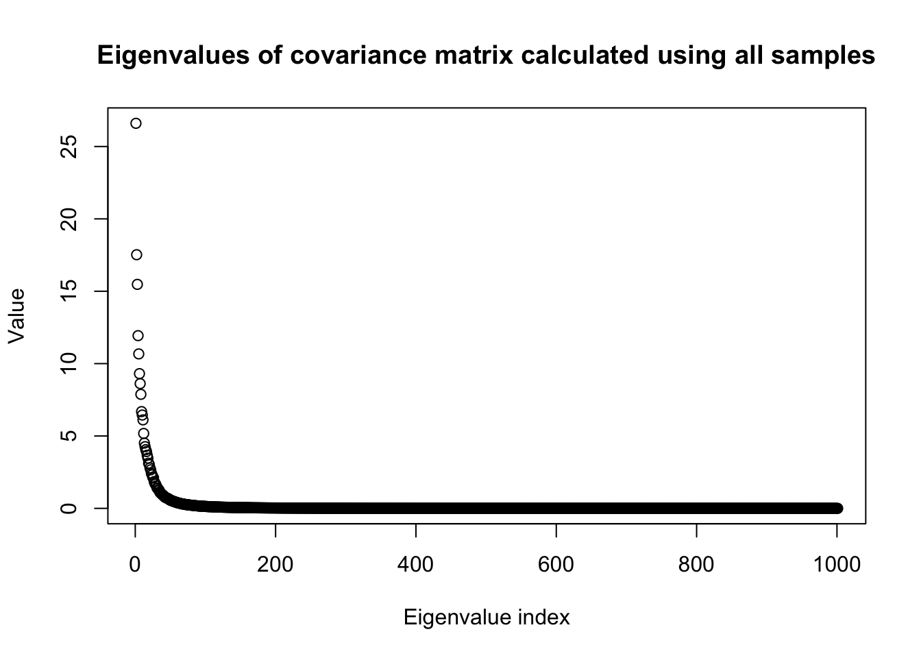
| Version | Author | Date |
|---|---|---|
| 7edf83c | dodat97 | 2025-12-02 |
n0 = dim(X0)[1]
p0 = dim(X0)[2]
snp_total = p0
We proceed to split the data into half and look at the heatmap of the covariance matrices of two sub-samples.
#### randomly split the data into half
#### randomly select p consecutive SNPs where p < n so IW is proper
p = 100
# Start from a random point on the genome
indx_start = sample(1: (snp_total - p), 1)
X = X0[, indx_start:(indx_start + p -1)]
# View(cor(X)[1:10, 1:10])
## sub-sample into two
out_sample_size = n0 / 2
out_sample = sample(1:n0, out_sample_size)
X_out = X[out_sample, ]
X_in = X[setdiff(1:n0, out_sample), ]

rm_p = c(which(diag(cov(X_in))==0), which(diag(cov(X_out))==0))
indx_p = setdiff(1:p, rm_p)
X_in = X_in[, indx_p]
X_out = X_out[, indx_p]
## out-sample LD matrix
p = length(indx_p)
Rp = cov(X_out)
R0 = cov(X_in)
library(ggplot2)
library(reshape2)
df1 <- melt(R0)
df2 <- melt(Rp)
N_in = nrow(X_in)
N_out = nrow(X_out)
p1 <- ggplot(df1, aes(Var1, Var2, fill = value)) +
  geom_tile() +
  scale_fill_gradient2(low="blue", mid="white", high="red") +
  coord_fixed() +
  ggtitle(sprintf("In-sample Cov, %d samples", nrow(X_in)))
p2 <- ggplot(df2, aes(Var1, Var2, fill = value)) +
  geom_tile() +
  scale_fill_gradient2(low="blue", mid="white", high="red") +
  coord_fixed() +
  ggtitle(sprintf("Out-of-sample Cov, %d samples", nrow(X_out)))
library(gridExtra)
grid.arrange(p1, p2, ncol = 2)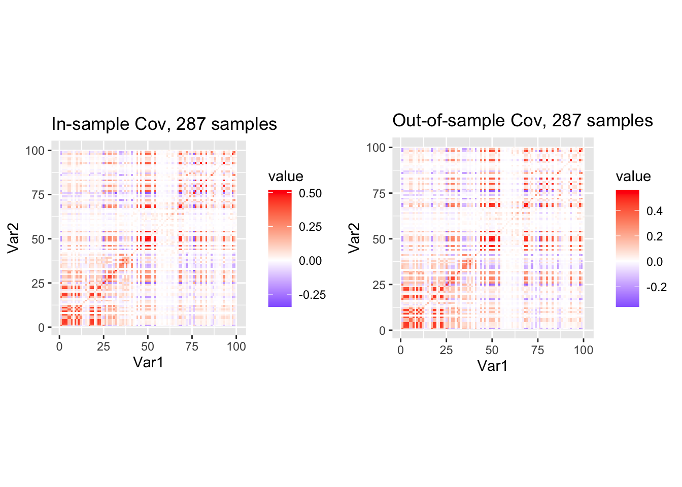
Log-likelihood functions:
## Matrix F-distribution likelihood
#### log F(R0 | nu * Rp / N, N, nu + 2)
log_multigamma_vec <- function(a, p) {
  # vectorized multivariate gamma
  shifts <- (1 - seq_len(p)) / 2
  # sum over j, but broadcasting a over j
  (p*(p-1)/4)*log(pi) +
    rowSums(lgamma(outer(a, shifts, "+")))
}


log_F <- function(R0, Rp, N, nu_vec) {
  p <- nrow(R0)
  jitter = 1e-8
  R0 = R0 + jitter * diag(p)
  Rp = Rp + jitter * diag(p)
  # Precompute expensive shared quantities
  logdet_nu_Rp_over_N <- (determinant(Rp, logarithm = TRUE)$modulus
                          + p * log(nu_vec)
                          - p * log(N))
  logdetR0   <- determinant(R0, logarithm = TRUE)$modulus

  # lambda_vec <- eigen(solve(Rp, R0))$values
  # lambda_over_nu = tcrossprod(lambda_vec, N / nu_vec)
  # logdet_I_plus_RR <- colSums(log(1 + lambda_over_nu))
  # llhs = (log_multigamma_vec((N + nu_vec + p + 1) / 2, p)
  #         - log_multigamma_vec(N / 2, p)
  #         - log_multigamma_vec((nu_vec + p + 1) / 2, p)
  #         - .5 * N * logdet_nu_Rp_over_N
  #         + .5 * (N - p - 1) * logdetR0
  #         - .5 * (N + nu_vec + p + 1) * logdet_I_plus_RR)

  logdet_Rplus_Rp = rep(0, length(nu_vec))
  for (idx in 1:length(nu_vec)){
    nu = nu_vec[idx]
    logdet_Rplus_Rp[idx] <- determinant(R0 + nu * Rp / N, logarithm = TRUE)$modulus
  }

  llhs = (log_multigamma_vec((N + nu_vec + p + 1) / 2, p)
          - log_multigamma_vec(N / 2, p)
          - log_multigamma_vec((nu_vec + p + 1) / 2, p)
          + .5 * (nu_vec + p + 1) * logdet_nu_Rp_over_N
          + .5 * (N - p - 1) * logdetR0
          - .5 * (N + nu_vec + p + 1) * logdet_Rplus_Rp)

  as.numeric(llhs)
}

log_iw <- function(R0, Rp, nu_vec) {
  p <- nrow(R0)
  jitter = 1e-12
  R0 = R0 + jitter * diag(p)
  Rp = Rp + jitter * diag(p)
  # Precompute expensive shared quantities
  logdet_nu_Rp <- determinant(Rp, logarithm = TRUE)$modulus + p * log(nu_vec)
  logdetR0   <- determinant(R0,   logarithm = TRUE)$modulus
  tr_term   <- nu_vec * sum(t(Rp) * solve(R0))
  llhs = (.5 * (nu_vec + p + 1) * logdet_nu_Rp
          - .5 * (nu_vec + p + 1) * p * log(2)
          - log_multigamma_vec((nu_vec + p + 1) / 2, p)
          - .5 * (nu_vec + 2 * (p + 1)) * logdetR0
          - .5 * tr_term)
  as.numeric(llhs)
}
2. Comparing \(\nu\) learned in the considered models
Model 1
\[\mathcal{IW}(\Psi_{PCA} | \nu \Psi'_{PCA}, \nu + p + 1)\] This is not really a model for \(R_0\), but it gives largest \(\nu\).
eig <- eigen(Rp)
eig_cumsum = cumsum(eig$values)
percent_explained = .99
eig_cumsum = cumsum(eig$values)
q = sum(eig_cumsum < percent_explained * eig_cumsum[p])
sprintf("%d first principle components explain %.1f percent of variance", q, percent_explained*100)
[1] "40 first principle components explain 99.0 percent of variance"lambda <- eig$values
U <- eig$vectors
sigma2_est <- mean(lambda[(q+1):p])
L_diag <- sqrt(lambda[1:q] - sigma2_est)
# L_diag <- sqrt(lambda[1:q])
W_ppca <- U[,1:q] %*% diag(L_diag)
Rp_PCA <- W_ppca %*% t(W_ppca) + sigma2_est * diag(p)
eig <- eigen(R0)
lambda <- eig$values
U <- eig$vectors
sigma2_est <- mean(lambda[(q+1):p])
L_diag <- sqrt(lambda[1:q] - sigma2_est)
# L_diag <- sqrt(lambda[1:q])
W_ppca <- U[,1:q] %*% diag(L_diag)
R0_PCA <- W_ppca %*% t(W_ppca) + sigma2_est * diag(p)
nu_vec = c(1:100)
llhs = log_iw(R0_PCA, Rp_PCA, nu_vec)
# llhs = log_iw(R0_PCA, Rp, nu_vec)
# llhs = log_iw(R0, Rp_PCA, nu_vec)
plot(nu_vec, llhs, xlab = "nu value", ylab = "log-likelihood")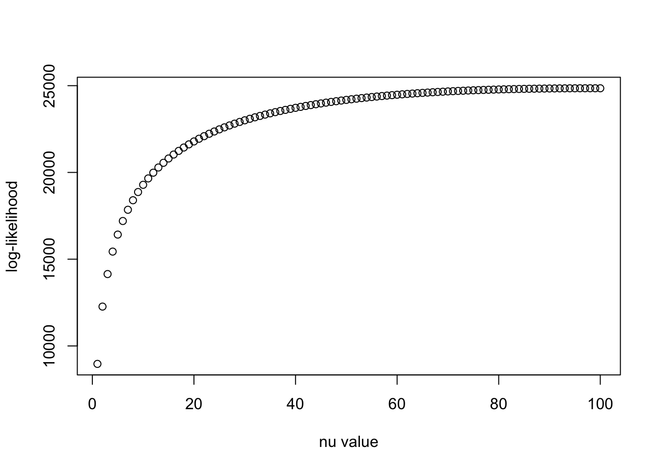
print(nu_vec[which.max(llhs)])[1] 98Model 2
\[\mathrm{F}(R_0 | \frac{\nu R'}{N}, N, \nu + 2)\] This model corresponds to the hierarchy \[R_0 | \Psi \sim \mathcal{W}(\Psi / N, N), \quad \Psi | R' \sim \mathcal{IW}(\nu R', \nu + p + 1).\]
N = nrow(X_in)
nu_vec = c(1:100)
llhs = log_F(R0, Rp, N, nu_vec)
plot(nu_vec, llhs, xlab = "nu value", ylab = "log-likelihood of matrix F-distribution")
print(paste0("Optimal nu is ", nu_vec[which.max(llhs)]))[1] "Optimal nu is 32"Model 3
\[\mathrm{F}(R_0 | \frac{\nu \Psi'}{N}, N, \nu + 2)\] This model corresponds to the hierarchy \[R_0 | \Psi \sim \mathcal{W}(\Psi / N, N), \quad \Psi | \Psi' \sim \mathcal{IW}(\nu \Psi', \nu + p + 1),\] and \(\Psi' = (N' R' + \delta I) / (N' + \delta)\) being the posterior mean of the estimated population covariance matrix.
N = nrow(X_in)
Np = nrow(X_out)
nu_vec = c(1:100)
delta = 1e-6
Psi_p = (Np * Rp + delta * diag(p)) / (Np + delta)
llhs = log_F(R0, Psi_p, N, nu_vec)
plot(nu_vec, llhs, xlab = "nu value", ylab = "log-likelihood of matrix F-distribution")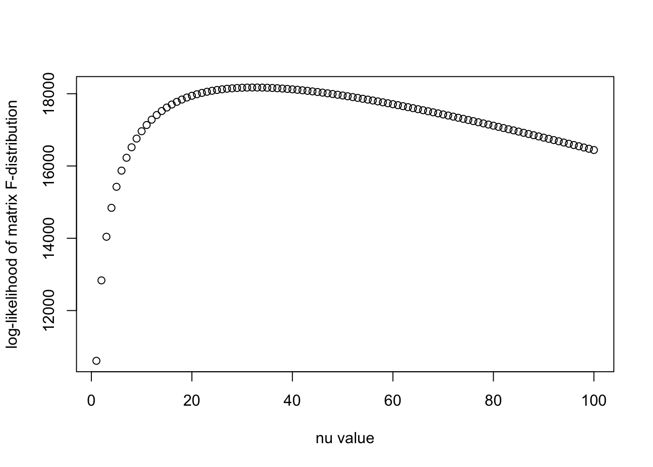
print(paste0("Optimal nu is ", nu_vec[which.max(llhs)]))[1] "Optimal nu is 32"Model 4
\[\mathrm{F}(R_0 | \frac{\nu \Psi_{PCA}'}{N}, N, \nu + 2)\]
nu_vec = c(1:100)

llhs = log_F(R0, Rp_PCA, N, nu_vec)
plot(nu_vec, llhs, xlab = "nu value", ylab = "log-likelihood of matrix F-distribution")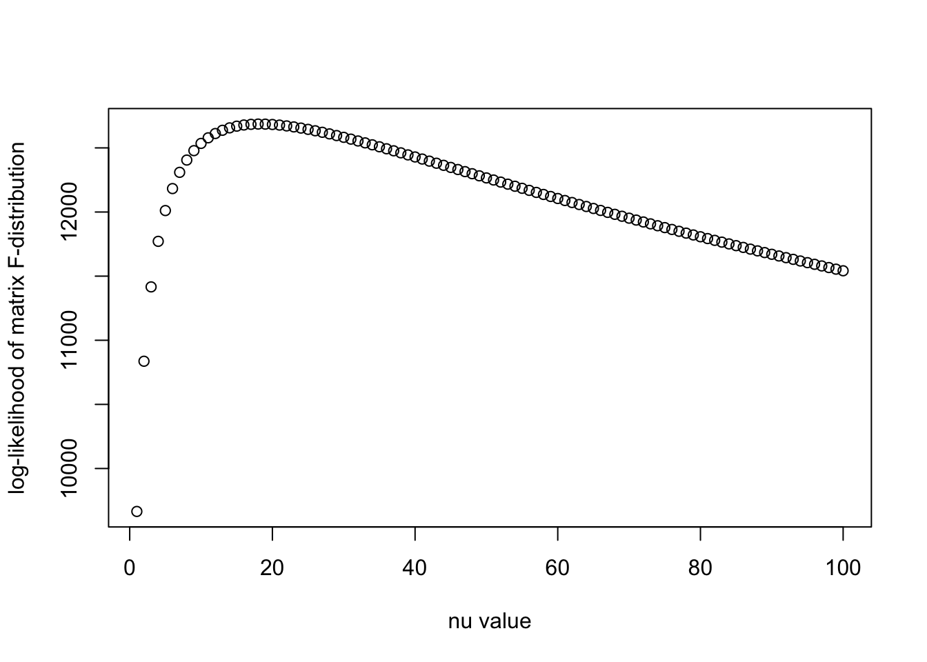
print(paste0("Optimal nu is ", nu_vec[which.max(llhs)]))[1] "Optimal nu is 18"Model 5
\[\mathrm{IW}(R_0 | \nu \Psi_{Bayes}', \nu + p + 1)\]
nu_vec = c(1:100)
llhs = log_iw(R0, Psi_p, nu_vec)
plot(nu_vec, llhs, xlab = "nu value", ylab = "log-likelihood")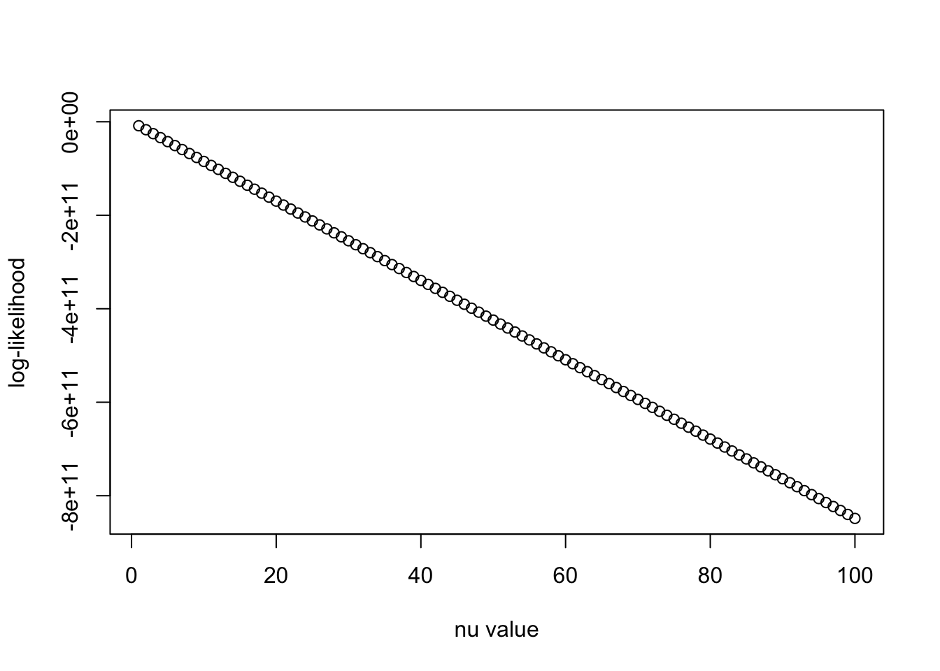
print(nu_vec[which.max(llhs)])[1] 1Model 6
Model 6: This is our original easiest model, but the estimated \(\nu\) in this model is very small \[\mathrm{IW}(R_0 | \nu R', \nu + p + 1)\]
nu_vec = c(1:100)
llhs = log_iw(R0, Rp, nu_vec)
plot(nu_vec, llhs, xlab = "nu value", ylab = "log-likelihood")
print(nu_vec[which.max(llhs)])[1] 1
sessionInfo()R version 4.3.2 (2023-10-31)
Platform: aarch64-apple-darwin20 (64-bit)
Running under: macOS 15.6.1
Matrix products: default
BLAS: /Library/Frameworks/R.framework/Versions/4.3-arm64/Resources/lib/libRblas.0.dylib
LAPACK: /Library/Frameworks/R.framework/Versions/4.3-arm64/Resources/lib/libRlapack.dylib; LAPACK version 3.11.0
locale:
[1] en_US.UTF-8/en_US.UTF-8/en_US.UTF-8/C/en_US.UTF-8/en_US.UTF-8
time zone: America/Chicago
tzcode source: internal
attached base packages:
[1] stats graphics grDevices utils datasets methods base
other attached packages:
[1] gridExtra_2.3 reshape2_1.4.5 ggplot2_4.0.1 Matrix_1.6-1.1
[5] susieR_0.14.2 workflowr_1.7.2
loaded via a namespace (and not attached):
[1] sass_0.4.10 generics_0.1.4 stringi_1.8.7 lattice_0.22-7
[5] digest_0.6.39 magrittr_2.0.4 evaluate_1.0.5 grid_4.3.2
[9] RColorBrewer_1.1-3 fastmap_1.2.0 plyr_1.8.9 rprojroot_2.1.1
[13] jsonlite_2.0.0 processx_3.8.6 whisker_0.4.1 reshape_0.8.10
[17] mixsqp_0.3-54 ps_1.9.1 promises_1.5.0 httr_1.4.7
[21] scales_1.4.0 jquerylib_0.1.4 cli_3.6.5 rlang_1.1.6
[25] crayon_1.5.3 withr_3.0.2 cachem_1.1.0 yaml_2.3.11
[29] otel_0.2.0 tools_4.3.2 dplyr_1.1.4 httpuv_1.6.16
[33] vctrs_0.6.5 R6_2.6.1 matrixStats_1.5.0 lifecycle_1.0.4
[37] git2r_0.36.2 stringr_1.6.0 fs_1.6.6 irlba_2.3.5.1
[41] pkgconfig_2.0.3 callr_3.7.6 pillar_1.11.1 bslib_0.9.0
[45] later_1.4.4 gtable_0.3.6 glue_1.8.0 Rcpp_1.1.0
[49] xfun_0.54 tibble_3.3.0 tidyselect_1.2.1 rstudioapi_0.17.1
[53] knitr_1.50 farver_2.1.2 htmltools_0.5.8.1 labeling_0.4.3
[57] rmarkdown_2.30 compiler_4.3.2 getPass_0.2-4 S7_0.2.1