Learning both degree-of-freedom in matrix F-distribution
Last updated: 2025-12-02
Checks: 7 0
Knit directory: Improved_LD_SuSiE/
This reproducible R Markdown analysis was created with workflowr (version 1.7.1). The Checks tab describes the reproducibility checks that were applied when the results were created. The Past versions tab lists the development history.
Great! Since the R Markdown file has been committed to the Git repository, you know the exact version of the code that produced these results.
Great job! The global environment was empty. Objects defined in the global environment can affect the analysis in your R Markdown file in unknown ways. For reproduciblity it’s best to always run the code in an empty environment.
The command set.seed(20250821) was run prior to running
the code in the R Markdown file. Setting a seed ensures that any results
that rely on randomness, e.g. subsampling or permutations, are
reproducible.
Great job! Recording the operating system, R version, and package versions is critical for reproducibility.
Nice! There were no cached chunks for this analysis, so you can be confident that you successfully produced the results during this run.
Great job! Using relative paths to the files within your workflowr project makes it easier to run your code on other machines.
Great! You are using Git for version control. Tracking code development and connecting the code version to the results is critical for reproducibility.
The results in this page were generated with repository version 384612e. See the Past versions tab to see a history of the changes made to the R Markdown and HTML files.
Note that you need to be careful to ensure that all relevant files for
the analysis have been committed to Git prior to generating the results
(you can use wflow_publish or
wflow_git_commit). workflowr only checks the R Markdown
file, but you know if there are other scripts or data files that it
depends on. Below is the status of the Git repository when the results
were generated:
Ignored files:
    Ignored:    .DS_Store
    Ignored:    .RData
    Ignored:    .Rhistory
    Ignored:    analysis/.RData
    Ignored:    analysis/.Rhistory

Unstaged changes:
    Modified:   analysis/index.Rmd
    Modified:   code_push.R
Note that any generated files, e.g. HTML, png, CSS, etc., are not included in this status report because it is ok for generated content to have uncommitted changes.
These are the previous versions of the repository in which changes were
made to the R Markdown (analysis/learn-N-nu-jointly.Rmd)
and HTML (docs/learn-N-nu-jointly.html) files. If you’ve
configured a remote Git repository (see ?wflow_git_remote),
click on the hyperlinks in the table below to view the files as they
were in that past version.
| File | Version | Author | Date | Message |
|---|---|---|---|---|
| Rmd | 384612e | dodat97 | 2025-12-02 | wflow_publish(c("analysis/learn-N-nu-jointly.Rmd")) |
In the previous Markdown, we see that the model \[R^{(0)} \sim \mathrm{F}\left(\dfrac{\nu \Psi^{(1)}}{N}, N, \nu + 2\right),\] gives a not-too-small estimate of \(\nu\), where \(R^{(0)}\) is the in-sample covariance matrix, and \(\Psi^{(1)}\) is the out-of-sample population covarance matrix estimated from a Bayesian procedure from the out-of-sample covariance matrix \(R^{(1)}\).
In this Markdown, we will try varying both the degree-of-freedom \(N\) and \(\nu\) to see if we can have a different estimate of \(\nu\). Note that when varying both of them, this distribution still has mean \(\Psi^{(1)}\).
1. Data preparation and log-likelihood functions
First, load the data:
seed = 10  ## change this to see different experiment
set.seed(seed)
library(susieR)
library(Matrix)

data(N3finemapping)
attach(N3finemapping)
X0 = N3finemapping$X
## getting covariance matrix from the whole sample
## and examine the eigendecomposition to estimate numerical rank
R = cov(X0)
eig <- eigen(R)
plot(eig$values,
     main = "Eigenvalues of covariance matrix calculated using all samples",
     ylab = "Value",
     xlab = "Eigenvalue index")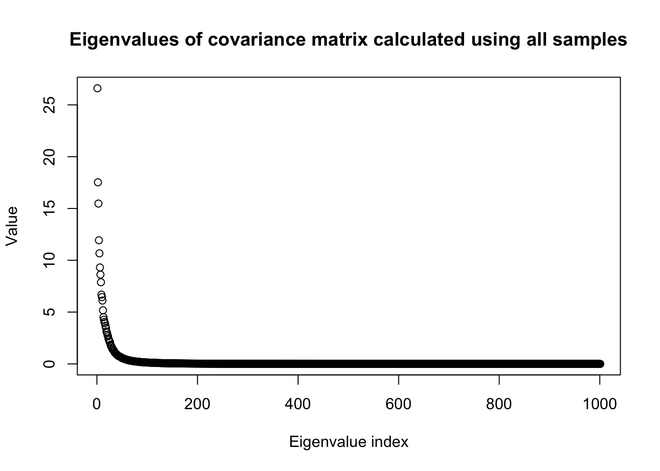
n0 = dim(X0)[1]
p0 = dim(X0)[2]
snp_total = p0
We proceed to split the data into half and look at the heatmap of the covariance matrices of two sub-samples.
#### randomly split the data into half
#### randomly select p consecutive SNPs where p < n so IW is proper
p = 100
# Start from a random point on the genome
indx_start = sample(1: (snp_total - p), 1)
X = X0[, indx_start:(indx_start + p -1)]
# View(cor(X)[1:10, 1:10])
## sub-sample into two
out_sample_size = n0 / 2
out_sample = sample(1:n0, out_sample_size)
X_out = X[out_sample, ]
X_in = X[setdiff(1:n0, out_sample), ]

rm_p = c(which(diag(cov(X_in))==0), which(diag(cov(X_out))==0))
indx_p = setdiff(1:p, rm_p)
X_in = X_in[, indx_p]
X_out = X_out[, indx_p]
## out-sample LD matrix
p = length(indx_p)
Rp = cov(X_out)
R0 = cov(X_in)
library(ggplot2)
library(reshape2)
df1 <- melt(R0)
df2 <- melt(Rp)
N_in = nrow(X_in)
N_out = nrow(X_out)
p1 <- ggplot(df1, aes(Var1, Var2, fill = value)) +
  geom_tile() +
  scale_fill_gradient2(low="blue", mid="white", high="red") +
  coord_fixed() +
  ggtitle(sprintf("In-sample Cov, %d samples", nrow(X_in)))
p2 <- ggplot(df2, aes(Var1, Var2, fill = value)) +
  geom_tile() +
  scale_fill_gradient2(low="blue", mid="white", high="red") +
  coord_fixed() +
  ggtitle(sprintf("Out-of-sample Cov, %d samples", nrow(X_out)))
library(gridExtra)
grid.arrange(p1, p2, ncol = 2)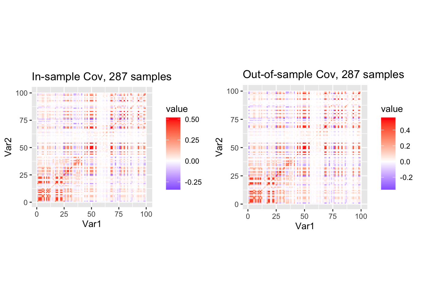
Log-likelihood functions:
## Matrix F-distribution likelihood
#### log F(R0 | nu * Psi1 / N, N, nu + 2)

### vectorize log multivariate Gamma function
log_multigamma_vec <- function(A, p) {
  if (!is.matrix(A)) A <- as.matrix(A)
  shifts <- (1 - seq_len(p)) / 2

  # Check domain: a + (1-k)/2 must be > 0 (or > -Inf for complex) for lgamma defined
  min_allowed <- (p - 1) / 2
  if (any(A <= min_allowed - 1e-12)) {
    stop(sprintf("Entries of A must satisfy Re(a) > (p-1)/2 = %g", min_allowed))
  }

  # sapply returns an array of dim m x n x p when the FUN returns an m x n matrix
  terms_lgamma <- sapply(shifts, function(s) lgamma(A + s), simplify = "array")

  S <- apply(terms_lgamma, c(1, 2), sum)
  const <- p * (p - 1) / 4 * log(pi)
  S + const
}


log_F_matrix <- function(R0, Psi1, N_vec, nu_vec) {
  p <- nrow(R0)
  jitter = 1e-8
  R0 = R0 + jitter * diag(p)
  n = length(N_vec)
  m = length(nu_vec)

  logdet_nu_Rp_over_N <- (determinant(Psi1, logarithm = TRUE)$modulus
                          + p * outer(- log(N_vec), log(nu_vec), "+"))  ## (n, m)
  power_Rp = - .5 * matrix(rep(N_vec, m), nrow=n)  ## (n, m)
  first_term = power_Rp * logdet_nu_Rp_over_N

  logdetR0 <- determinant(R0, logarithm = TRUE)$modulus
  power_R0 <- .5 * matrix(rep(N_vec - p - 1, m), nrow=n)
  second_term = power_R0 * logdetR0

  lambda_vec <- Re(eigen(solve(Psi1, R0))$values)  ## (p)
  lambda_N_over_nu = N_vec %o% (1 / nu_vec) %o% lambda_vec
  logdet_I_plus_RR <- apply(log(1 + lambda_N_over_nu), c(1, 2), sum)
  power_RR = - .5 * (outer(N_vec, nu_vec, "+") + p + 1)
  third_term = power_RR * logdet_I_plus_RR

  constant_term1 = log_multigamma_vec((outer(N_vec, nu_vec, "+") + p + 1) / 2 , p)
  constant_term2 = - log_multigamma_vec(matrix(rep(N_vec, m), nrow=n) / 2 , p)
  constant_term3 = - log_multigamma_vec(matrix(rep(nu_vec + p + 1, n), nrow=n, byrow=TRUE) / 2 , p)

  llhs = (constant_term1 + constant_term2 + constant_term3
          + first_term + second_term + third_term)

  return(llhs)
}

log_iw <- function(R0, Rp, nu_vec) {
  p <- nrow(R0)
  jitter = 1e-12
  R0 = R0 + jitter * diag(p)
  Rp = Rp + jitter * diag(p)
  # Precompute expensive shared quantities
  logdet_nu_Rp <- determinant(Rp, logarithm = TRUE)$modulus + p * log(nu_vec)
  logdetR0   <- determinant(R0,   logarithm = TRUE)$modulus
  tr_term   <- nu_vec * sum(t(Rp) * solve(R0))
  llhs = (.5 * (nu_vec + p + 1) * logdet_nu_Rp
          - .5 * (nu_vec + p + 1) * p * log(2)
          - log_multigamma_vec((nu_vec + p + 1) / 2, p)
          - .5 * (nu_vec + 2 * (p + 1)) * logdetR0
          - .5 * tr_term)
  as.numeric(llhs)
}
2. Learn both \(N\) and \(\nu\)
Model
\[\mathcal{IW}(\Psi_{PCA} | \nu \Psi'_{PCA}, \nu + p + 1)\] This is not really a model for \(R_0\), but it gives largest \(\nu\).
N = nrow(X_in)
Np = nrow(X_out)
# N_vec = c((p+1):(N+p))
N_vec = c(p:N)
nu_vec = c(1:100)
delta = 1e-6
Psi1 = (Np * Rp + delta * diag(p)) / (Np + delta)
llhs = log_F_matrix(R0, Psi1, N_vec, nu_vec)

library(ggplot2)
library(reshape2)

df <- melt(llhs, varnames = c("N", "nu"), value.name = "value")

ggplot(df, aes(x = nu, y = N, fill = value)) +
  geom_tile() +
  scale_fill_gradient2(low = "blue", high = "red", mid = "white") +
  theme_minimal() +
  labs(x = "nu", y = "N - p + 1", fill = "Log-likelihood")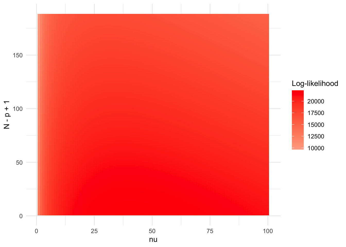
nu_max_each_N = max.col(llhs, ties.method = "first")

nu_max_each_N
[1] 41 41 41 41 41 41 41 41 41 41 40 40 40 40 40 40 40 40 40 40 40 40 40 40 40
[26] 40 40 40 40 39 39 39 39 39 39 39 39 39 39 39 39 39 39 39 39 39 38 38 38 38
[51] 38 38 38 38 38 38 38 38 38 38 38 38 38 37 37 37 37 37 37 37 37 37 37 37 37
[76] 37 37 37 37 37 36 36 36 36 36 36 36 36 36 36 36 36 36 36 36 36 36 35 35 35
[101] 35 35 35 35 35 35 35 35 35 35 35 35 35 35 34 34 34 34 34 34 34 34 34 34 34
[126] 34 34 34 34 34 33 33 33 33 33 33 33 33 33 33 33 33 33 33 33 33 33 32 32 32
[151] 32 32 32 32 32 32 32 32 32 32 32 32 32 32 32 31 31 31 31 31 31 31 31 31 31
[176] 31 31 31 31 31 31 31 30 30 30 30 30 30log_multigamma_v <- function(a, p) {
# vectorized multivariate gamma
j <- 1:p
# sum over j, but broadcasting a over j
(p*(p-1)/4)*log(pi) +
rowSums(matrix(lgamma(a), nrow=length(a), ncol=p, byrow=FALSE) +
matrix((1 - j)/2, nrow=length(a), ncol=p, byrow=TRUE))
}
log_F <- function(R0, Rp, N, nu_vec) {
p <- nrow(R0)
jitter = 1e-8
R0 = R0 + jitter * diag(p)
# Precompute expensive shared quantities
logdet_nu_Rp_over_N <- (determinant(Rp, logarithm = TRUE)$modulus
+ p * log(nu_vec)
- p * log(N))
logdetR0 <- determinant(R0, logarithm = TRUE)$modulus
lambda_vec <- eigen(solve(Rp, R0))$values
lambda_over_nu = tcrossprod(lambda_vec, N / nu_vec)
logdet_I_plus_RR <- colSums(log(1 + lambda_over_nu))
llhs = (log_multigamma_v((N + nu_vec + p + 1) / 2, p)
- log_multigamma_v(N / 2, p)
- log_multigamma_v((nu_vec + p + 1) / 2, p)
- .5 * N * logdet_nu_Rp_over_N
+ .5 * (N - p - 1) * logdetR0
- .5 * (N + nu_vec + p + 1) * logdet_I_plus_RR)
# logdet_Rplus_Rp = rep(0, length(nu_vec))
# for (idx in 1:length(nu_vec)){
# nu = nu_vec[idx]
# logdet_Rplus_Rp[idx] <- determinant(R0 + nu * Rp / N, logarithm = TRUE)$modulus
# }
#
# llhs = (log_multigamma_v((N + nu_vec + p + 1) / 2, p)
# - log_multigamma_v(N / 2, p)
# - log_multigamma_v((nu_vec + p + 1) / 2, p)
# + .5 * (nu_vec + p + 1) * logdet_nu_Rp_over_N
# + .5 * (N - p - 1) * logdetR0
# - .5 * (N + nu_vec + p + 1) * logdet_Rplus_Rp)
#
as.numeric(llhs)
}
N = nrow(X_in)
llhs = log_F(R0, Psi1, N, nu_vec)
plot(nu_vec, llhs, xlab = "nu value", ylab = "log-likelihood")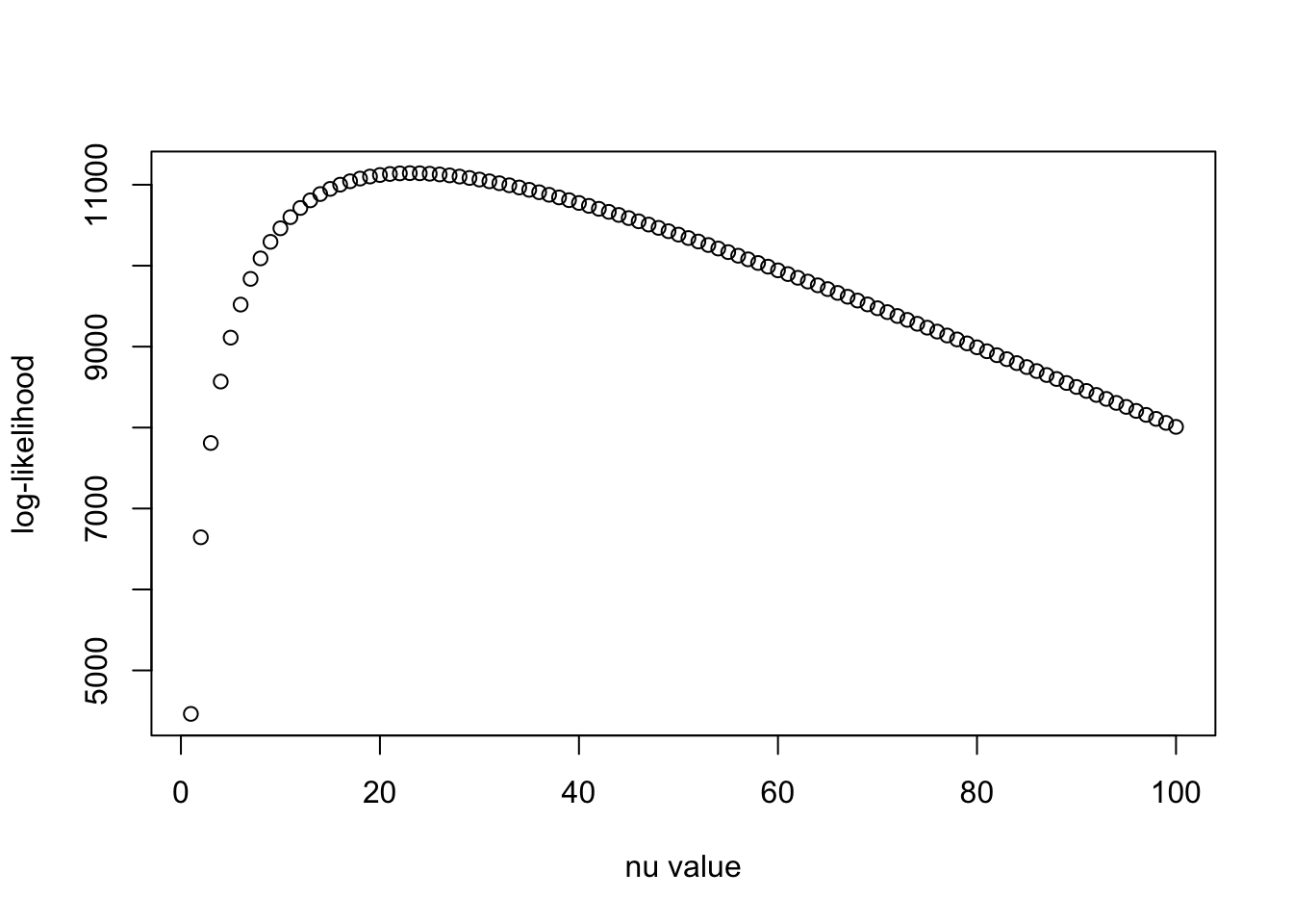
print(nu_vec[which.max(llhs)])[1] 23
sessionInfo()R version 4.5.1 (2025-06-13)
Platform: aarch64-apple-darwin20
Running under: macOS Sequoia 15.6.1
Matrix products: default
BLAS: /Library/Frameworks/R.framework/Versions/4.5-arm64/Resources/lib/libRblas.0.dylib
LAPACK: /Library/Frameworks/R.framework/Versions/4.5-arm64/Resources/lib/libRlapack.dylib; LAPACK version 3.12.1
locale:
[1] en_US.UTF-8/en_US.UTF-8/en_US.UTF-8/C/en_US.UTF-8/en_US.UTF-8
time zone: America/Chicago
tzcode source: internal
attached base packages:
[1] stats graphics grDevices utils datasets methods base
other attached packages:
[1] gridExtra_2.3 reshape2_1.4.4 ggplot2_3.5.2 Matrix_1.7-3
[5] susieR_0.14.2 workflowr_1.7.1
loaded via a namespace (and not attached):
[1] sass_0.4.10 generics_0.1.4 stringi_1.8.7 lattice_0.22-7
[5] digest_0.6.37 magrittr_2.0.3 evaluate_1.0.4 grid_4.5.1
[9] RColorBrewer_1.1-3 fastmap_1.2.0 plyr_1.8.9 rprojroot_2.1.0
[13] jsonlite_2.0.0 processx_3.8.6 whisker_0.4.1 reshape_0.8.10
[17] ps_1.9.1 mixsqp_0.3-54 promises_1.3.3 httr_1.4.7
[21] scales_1.4.0 jquerylib_0.1.4 cli_3.6.5 rlang_1.1.6
[25] crayon_1.5.3 withr_3.0.2 cachem_1.1.0 yaml_2.3.10
[29] tools_4.5.1 dplyr_1.1.4 httpuv_1.6.16 vctrs_0.6.5
[33] R6_2.6.1 matrixStats_1.5.0 lifecycle_1.0.4 git2r_0.36.2
[37] stringr_1.5.1 fs_1.6.6 irlba_2.3.5.1 pkgconfig_2.0.3
[41] callr_3.7.6 pillar_1.11.0 bslib_0.9.0 later_1.4.2
[45] gtable_0.3.6 glue_1.8.0 Rcpp_1.1.0 xfun_0.52
[49] tibble_3.3.0 tidyselect_1.2.1 rstudioapi_0.17.1 knitr_1.50
[53] farver_2.1.2 htmltools_0.5.8.1 labeling_0.4.3 rmarkdown_2.29
[57] compiler_4.5.1 getPass_0.2-4