Investigate learn degree-of-freedom nu
Last updated: 2025-11-24
Checks: 6 1
Knit directory: Improved_LD_SuSiE/
This reproducible R Markdown analysis was created with workflowr (version 1.7.1). The Checks tab describes the reproducibility checks that were applied when the results were created. The Past versions tab lists the development history.
Great! Since the R Markdown file has been committed to the Git repository, you know the exact version of the code that produced these results.
Great job! The global environment was empty. Objects defined in the global environment can affect the analysis in your R Markdown file in unknown ways. For reproduciblity it’s best to always run the code in an empty environment.
The command set.seed(20250821) was run prior to running
the code in the R Markdown file. Setting a seed ensures that any results
that rely on randomness, e.g. subsampling or permutations, are
reproducible.
Great job! Recording the operating system, R version, and package versions is critical for reproducibility.
Nice! There were no cached chunks for this analysis, so you can be confident that you successfully produced the results during this run.
Using absolute paths to the files within your workflowr project makes it difficult for you and others to run your code on a different machine. Change the absolute path(s) below to the suggested relative path(s) to make your code more reproducible.
| absolute | relative |
|---|---|
| ~/Documents/Improved_LD_SuSiE | . |
Great! You are using Git for version control. Tracking code development and connecting the code version to the results is critical for reproducibility.
The results in this page were generated with repository version ab50325. See the Past versions tab to see a history of the changes made to the R Markdown and HTML files.
Note that you need to be careful to ensure that all relevant files for
the analysis have been committed to Git prior to generating the results
(you can use wflow_publish or
wflow_git_commit). workflowr only checks the R Markdown
file, but you know if there are other scripts or data files that it
depends on. Below is the status of the Git repository when the results
were generated:
Unstaged changes:
    Modified:   code_push.R
Note that any generated files, e.g. HTML, png, CSS, etc., are not included in this status report because it is ok for generated content to have uncommitted changes.
These are the previous versions of the repository in which changes were
made to the R Markdown (analysis/investigate-df-nu.Rmd) and
HTML (docs/investigate-df-nu.html) files. If you’ve
configured a remote Git repository (see ?wflow_git_remote),
click on the hyperlinks in the table below to view the files as they
were in that past version.
| File | Version | Author | Date | Message |
|---|---|---|---|---|
| Rmd | ab50325 | dodat97 | 2025-11-24 | wflow_publish(c("analysis/investigate-df-nu.Rmd")) |
| html | 701ab1e | dodat | 2025-11-24 | Build site. |
| Rmd | 542074c | dodat | 2025-11-24 | wflow_publish(c("analysis/investigate-df-nu.Rmd")) |
| html | eba6c95 | dodat | 2025-11-23 | Build site. |
| Rmd | 0289377 | dodat | 2025-11-23 | add file |
seed = 4  ## change this value to see other examples
library(susieR)
library(Matrix)
set.seed(seed)
setwd("~/Documents/Improved_LD_SuSiE")
gtex = readRDS("data/Thyroid_ENSG00000132855.rds")
maf = apply(gtex, 2, function(x) sum(x)/2/length(x))
X0 = gtex[, maf > 0.01]
dim(X0)
[1] 574 7154X = na.omit(X0)
snp_total = ncol(X0)
n = nrow(X0)
p = 30
# Start from a random point on the genome
indx_start = sample(1: (snp_total - p), 1)
X = X0[, indx_start:(indx_start + p -1)]
# View(cor(X)[1:10, 1:10])
## sub-sample into two
out_sample_size = 250
out_sample = sample(1:n, out_sample_size)
X_out = X[out_sample, ]
X_in = X[setdiff(1:n, out_sample), ]
rm_p = c(which(diag(cov(X_in))==0), which(diag(cov(X_out))==0))
indx_p = setdiff(1:p, rm_p)
X_in = X_in[, indx_p]
X_out = X_out[, indx_p]
## out-sample LD matrix
p = length(indx_p)
Rp = cov(X_out)
R0 = cov(X_in)
library(ggplot2)
library(reshape2)
df1 <- melt(R0)
df2 <- melt(Rp)
N_in = nrow(X_in)
N_out = nrow(X_out)
p1 <- ggplot(df1, aes(Var1, Var2, fill = value)) +
geom_tile() +
scale_fill_gradient2(low="blue", mid="white", high="red") +
coord_fixed() +
ggtitle(paste0("In-sample Cov, sample =", nrow(X_in)))
p2 <- ggplot(df2, aes(Var1, Var2, fill = value)) +
geom_tile() +
scale_fill_gradient2(low="blue", mid="white", high="red") +
coord_fixed() +
ggtitle(paste0("Out-of-sample Cov, sample =", nrow(X_out)))
library(gridExtra)
grid.arrange(p1, p2, ncol = 2)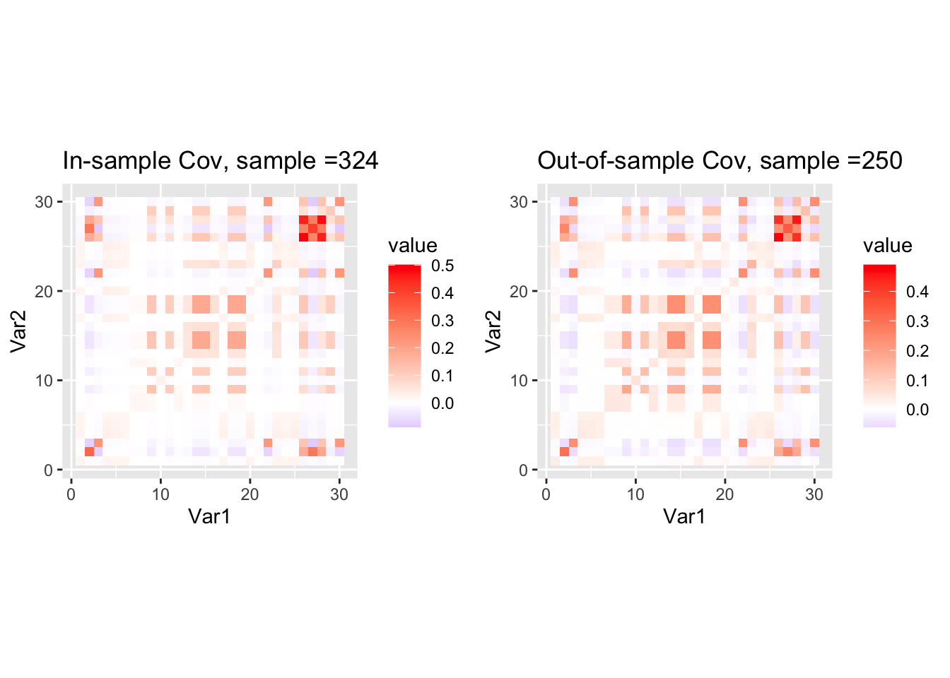
The in-sample R0 and out-of-sample Rp look pretty similar. Now let us plot the log density \(IW(R_0 | \nu R', \nu + p + 1)\) for various \(\nu\)
#### log IW(R0 | nu0 * Rp, nu0 + J + 1)
log_multigamma_vec <- function(a, p) {
  # vectorized multivariate gamma
  j <- 1:p
  # sum over j, but broadcasting a over j
  (p*(p-1)/4)*log(pi) +
    rowSums(matrix(lgamma(a), nrow=length(a), ncol=p, byrow=FALSE) +
              matrix((1 - j)/2, nrow=length(a), ncol=p, byrow=TRUE))
}

log_iw <- function(R0, Rp, nu_vec) {
  p <- nrow(R0)
  jitter = 1e-6
  R0 = R0 + jitter * diag(rep(1, p))
  Rp = Rp + jitter * diag(rep(1, p))
  # Precompute expensive shared quantities
  logdet_nu_Rp <- determinant(Rp, logarithm = TRUE)$modulus + p * log(nu_vec)
  logdetR0   <- determinant(R0,   logarithm = TRUE)$modulus
  tr_term   <- nu_vec * sum(t(Rp) * solve(R0))
  llhs = (.5 * (nu_vec + p + 1) * logdet_nu_Rp
          - .5 * (nu_vec + p + 1) * p * log(2)
          - log_multigamma_vec((nu_vec + p + 1) / 2, p)
          - .5 * (nu_vec + 2 * (p + 1)) * logdetR0
          - .5 * tr_term)
  as.numeric(llhs)
}

nu_vec = c(1:100) / 10
llhs = log_iw(R0, Rp, nu_vec)
plot(nu_vec, llhs, xlab = "nu value", ylab = "log-likelihood")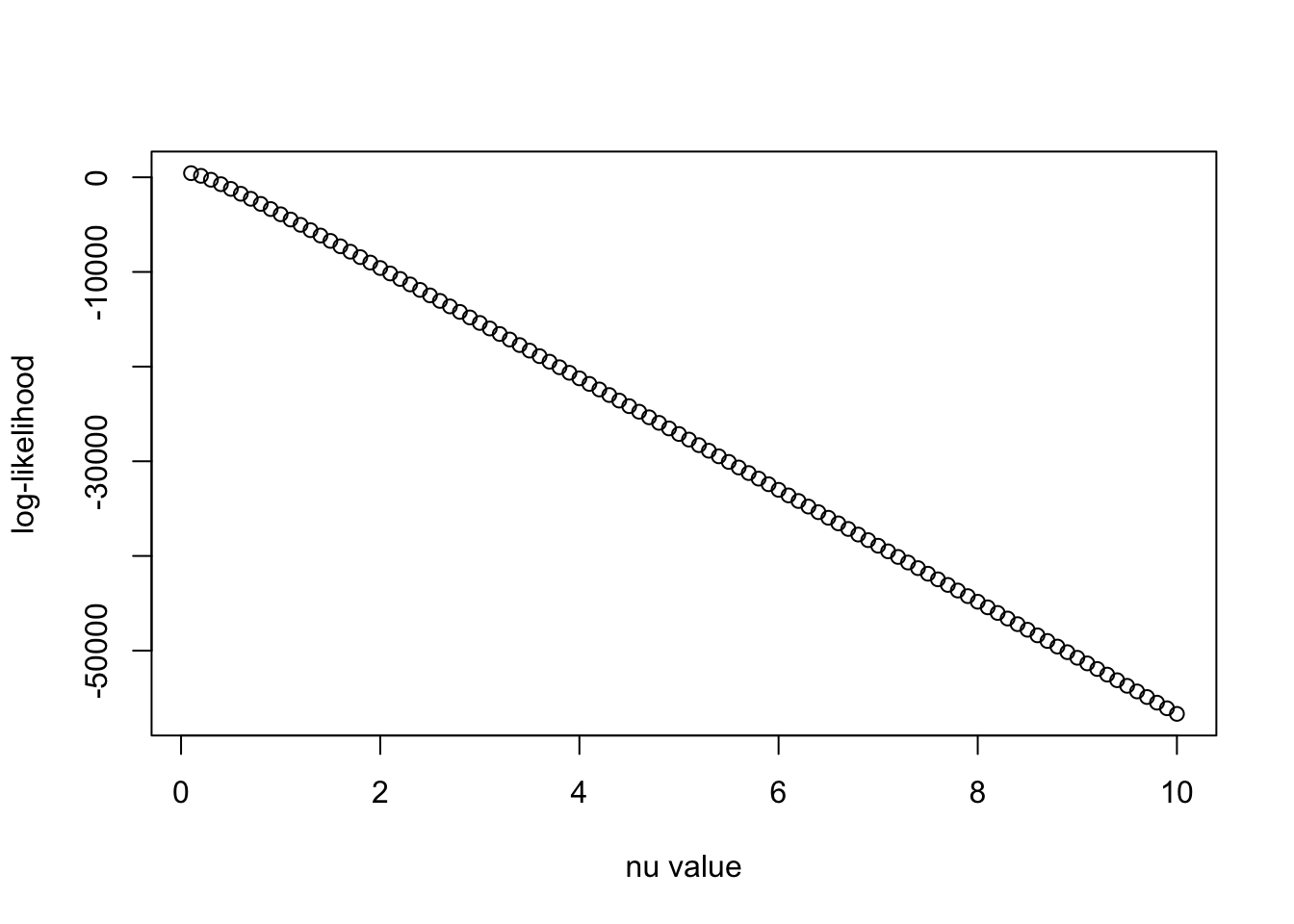
The trace term is too large compared to other term:
R0 = R0 + 1e-6 * diag(rep(1, p))
Rp = Rp + 1e-6 * diag(rep(1, p))
print(sum(t(Rp) * solve(R0))) ## trace term
[1] 11942.6determinant(R0, logarithm = TRUE)$modulus ## log det term[1] -202.9556
attr(,"logarithm")
[1] TRUEThis can be because both matrix R0 and Rp are almost low-rank (due to LD). Let us try two things (1) Plot the eigenvalues of R0 and Rp; (2) try this experiment again with full-rank population covariance matrix.
eig <- eigen(Rp)
plot(eig$values,
        main = "Eigenvalues of Rp",
        ylab = "Value",
        xlab = "Eigenvalue index")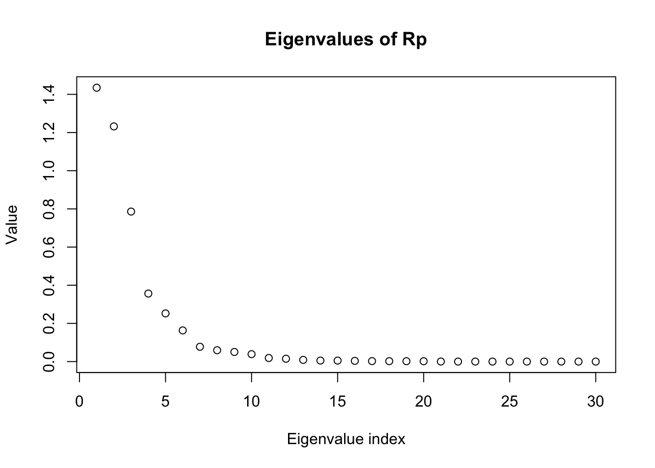
| Version | Author | Date |
|---|---|---|
| 701ab1e | dodat | 2025-11-24 |
print(eig$values) [1] 1.434889e+00 1.232171e+00 7.860183e-01 3.563626e-01 2.524908e-01
[6] 1.633243e-01 7.745190e-02 5.945554e-02 5.034201e-02 3.878367e-02
[11] 1.884320e-02 1.494342e-02 8.783745e-03 5.370828e-03 5.119441e-03
[16] 3.706699e-03 2.444832e-03 2.166237e-03 1.969695e-03 1.797069e-03
[21] 1.890547e-04 5.919595e-05 4.450706e-06 2.609377e-06 1.000000e-06
[26] 1.000000e-06 1.000000e-06 1.000000e-06 1.000000e-06 1.000000e-06- Let us try re-doing this experiment with the full-rank covariance matrix:
X_in = matrix(rnorm(N_in * p), nrow=N_in, ncol=p)
X_out = matrix(rnorm(N_out * p), nrow=N_out, ncol=p)
Rp = cov(X_out)
R0 = cov(X_in)
library(ggplot2)
library(reshape2)
df1 <- melt(R0)
df2 <- melt(Rp)
N_in = nrow(X_in)
N_out = nrow(X_out)
p1 <- ggplot(df1, aes(Var1, Var2, fill = value)) +
  geom_tile() +
  scale_fill_gradient2(low="blue", mid="white", high="red") +
  coord_fixed() +
  ggtitle(paste0("In-sample Cov, sample =", nrow(X_in)))
p2 <- ggplot(df2, aes(Var1, Var2, fill = value)) +
  geom_tile() +
  scale_fill_gradient2(low="blue", mid="white", high="red") +
  coord_fixed() +
  ggtitle(paste0("Out-of-sample Cov, sample =", nrow(X_out)))
library(gridExtra)
grid.arrange(p1, p2, ncol = 2)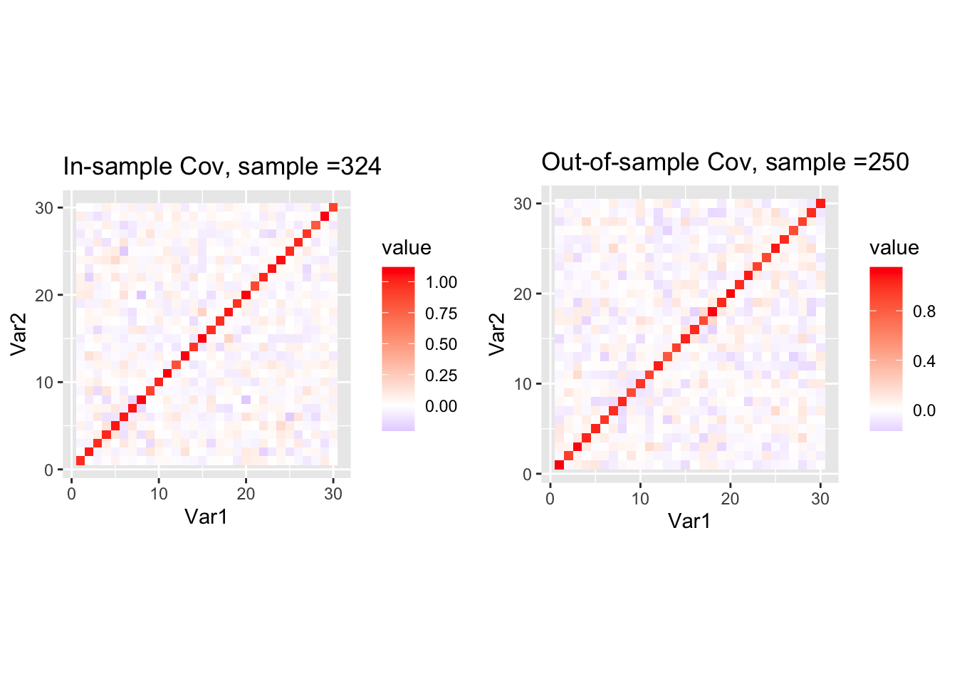
| Version | Author | Date |
|---|---|---|
| 701ab1e | dodat | 2025-11-24 |
nu_vec = c(1:100)
llhs = log_iw(R0, Rp, nu_vec)
plot(nu_vec, llhs, xlab = "nu value", ylab = "log-likelihood")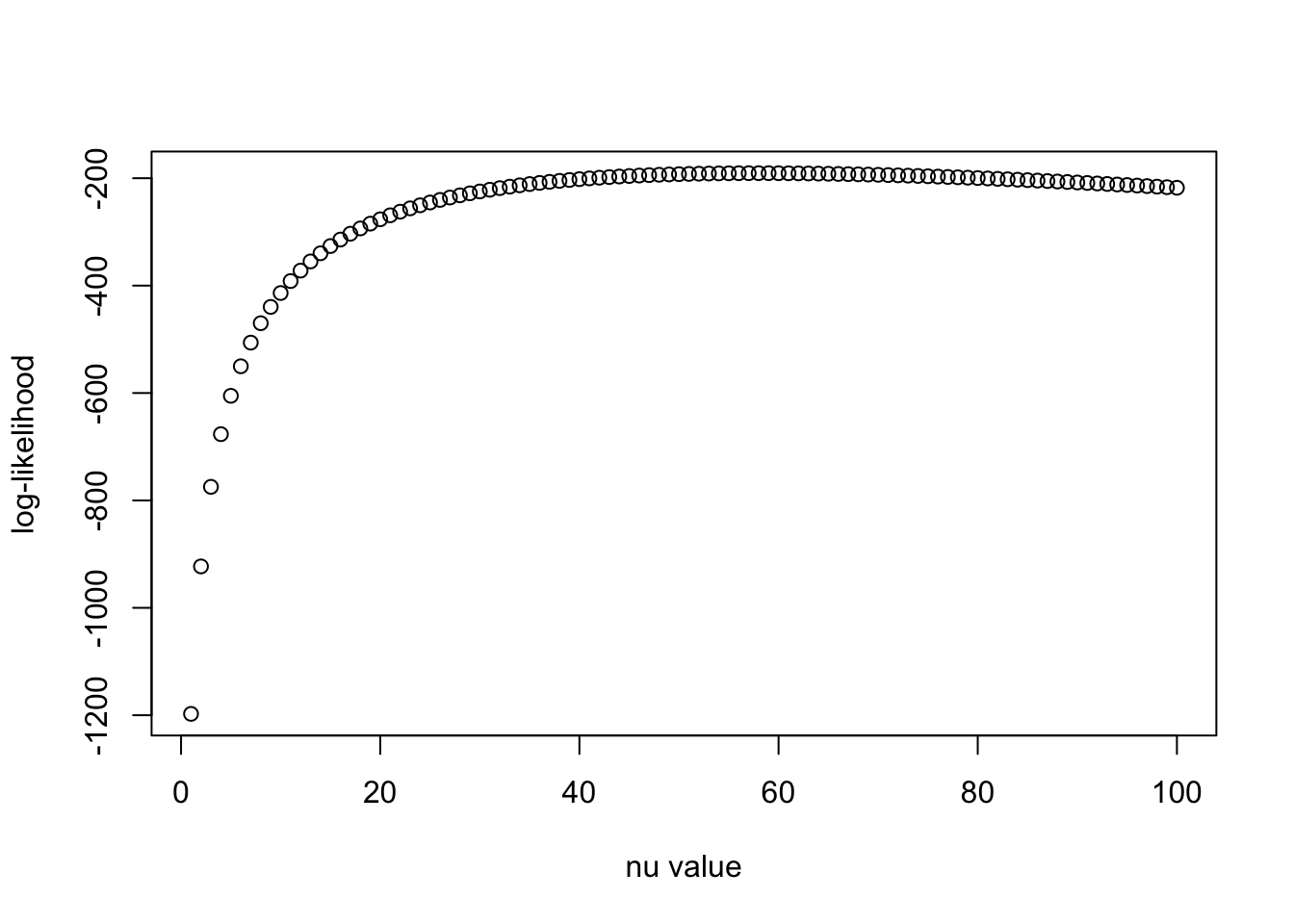
print(paste0("the optimal nu for full-rank R is ", nu_vec[which.max(llhs)]))[1] "the optimal nu for full-rank R is 58"TO-DO: (1) Try to vary rank \(r\) in the low-rank-plus-diag (2) Try to directly model the low-rank part of \(R\), i.e., set \(R = V C V^\top\) for \(R \in \mathbb{R}^{p\times r}\) and \(C \in \mathbb{R}^{r\times r}\) and model \(C\) by Inverse-Wishart instead of \(R\). (Does this corresponds to the generalized Inverse-Wishart?)
sessionInfo()R version 4.5.1 (2025-06-13)
Platform: aarch64-apple-darwin20
Running under: macOS Sequoia 15.6.1
Matrix products: default
BLAS: /Library/Frameworks/R.framework/Versions/4.5-arm64/Resources/lib/libRblas.0.dylib
LAPACK: /Library/Frameworks/R.framework/Versions/4.5-arm64/Resources/lib/libRlapack.dylib; LAPACK version 3.12.1
locale:
[1] en_US.UTF-8/en_US.UTF-8/en_US.UTF-8/C/en_US.UTF-8/en_US.UTF-8
time zone: America/Chicago
tzcode source: internal
attached base packages:
[1] stats graphics grDevices utils datasets methods base
other attached packages:
[1] gridExtra_2.3 reshape2_1.4.4 ggplot2_3.5.2 Matrix_1.7-3
[5] susieR_0.14.2 workflowr_1.7.1
loaded via a namespace (and not attached):
[1] sass_0.4.10 generics_0.1.4 stringi_1.8.7 lattice_0.22-7
[5] digest_0.6.37 magrittr_2.0.3 evaluate_1.0.4 grid_4.5.1
[9] RColorBrewer_1.1-3 fastmap_1.2.0 plyr_1.8.9 rprojroot_2.1.0
[13] jsonlite_2.0.0 processx_3.8.6 whisker_0.4.1 reshape_0.8.10
[17] ps_1.9.1 mixsqp_0.3-54 promises_1.3.3 httr_1.4.7
[21] scales_1.4.0 jquerylib_0.1.4 cli_3.6.5 rlang_1.1.6
[25] crayon_1.5.3 withr_3.0.2 cachem_1.1.0 yaml_2.3.10
[29] tools_4.5.1 dplyr_1.1.4 httpuv_1.6.16 vctrs_0.6.5
[33] R6_2.6.1 matrixStats_1.5.0 lifecycle_1.0.4 git2r_0.36.2
[37] stringr_1.5.1 fs_1.6.6 irlba_2.3.5.1 pkgconfig_2.0.3
[41] callr_3.7.6 pillar_1.11.0 bslib_0.9.0 later_1.4.2
[45] gtable_0.3.6 glue_1.8.0 Rcpp_1.1.0 xfun_0.52
[49] tibble_3.3.0 tidyselect_1.2.1 rstudioapi_0.17.1 knitr_1.50
[53] farver_2.1.2 htmltools_0.5.8.1 labeling_0.4.3 rmarkdown_2.29
[57] compiler_4.5.1 getPass_0.2-4