Last updated: 2025-08-31

Checks: 7 0

Knit directory: MTEB1Data/

This reproducible R Markdown analysis was created with workflowr (version 1.7.2). The Checks tab describes the reproducibility checks that were applied when the results were created. The Past versions tab lists the development history.

R Markdown file: up-to-date

Great! Since the R Markdown file has been committed to the Git repository, you know the exact version of the code that produced these results.

Environment: empty

Great job! The global environment was empty. Objects defined in the global environment can affect the analysis in your R Markdown file in unknown ways. For reproduciblity it’s best to always run the code in an empty environment.

Seed: set.seed(20250829)

The command set.seed(20250829) was run prior to running the code in the R Markdown file. Setting a seed ensures that any results that rely on randomness, e.g. subsampling or permutations, are reproducible.

Session information: recorded

Great job! Recording the operating system, R version, and package versions is critical for reproducibility.

Cache: none

Nice! There were no cached chunks for this analysis, so you can be confident that you successfully produced the results during this run.

File paths: relative

Great job! Using relative paths to the files within your workflowr project makes it easier to run your code on other machines.

Repository version: dc11ef4

Great! You are using Git for version control. Tracking code development and connecting the code version to the results is critical for reproducibility.

The results in this page were generated with repository version dc11ef4. See the Past versions tab to see a history of the changes made to the R Markdown and HTML files.

Note that you need to be careful to ensure that all relevant files for the analysis have been committed to Git prior to generating the results (you can use wflow_publish or wflow_git_commit). workflowr only checks the R Markdown file, but you know if there are other scripts or data files that it depends on. Below is the status of the Git repository when the results were generated:


Ignored files:
    Ignored:    .DS_Store
    Ignored:    .Rhistory
    Ignored:    .Rproj.user/
    Ignored:    analysis/.DS_Store
    Ignored:    data/.DS_Store

Untracked files:
    Untracked:  analysis/Introduction_to_CPLASS.Rmd
    Untracked:  analysis/figures/
    Untracked:  analysis/new_processed_stack.tif
    Untracked:  analysis/processed_stack.tif
    Untracked:  code/CPLASS.R
    Untracked:  code/Fill_missing_data.R
    Untracked:  code/PENALTY.R
    Untracked:  code/csa_functions.R
    Untracked:  code/msd_functions.R
    Untracked:  code/plot_functions.R
    Untracked:  code/postprocess.R
    Untracked:  data/CPLASS_MTEB1_1st.rds
    Untracked:  data/CPLASS_MTEB1_2nd.rds
    Untracked:  data/branch_points.csv
    Untracked:  data/branch_points.png
    Untracked:  data/first_approach_data.rds
    Untracked:  data/microtubles.png
    Untracked:  data/original_tracks_after_merging.rds
    Untracked:  data/processed_spots.csv
    Untracked:  data/second_approach_data.rds
    Untracked:  data/tracked_blobs.csv
    Untracked:  data/tracks_after_fill_in_missing_previous_method.rds

Note that any generated files, e.g. HTML, png, CSS, etc., are not included in this status report because it is ok for generated content to have uncommitted changes.

These are the previous versions of the repository in which changes were made to the R Markdown (analysis/Movement_analysis_on_MTEB1_data.Rmd) and HTML (docs/Movement_analysis_on_MTEB1_data.html) files. If you’ve configured a remote Git repository (see ?wflow_git_remote), click on the hyperlinks in the table below to view the files as they were in that past version.

File	Version	Author	Date	Message
html	466ea8e	Ldo3	2025-08-31	Build site.
Rmd	9449537	Ldo3	2025-08-31	wflow_publish(c("index.Rmd", "Movement_analysis_on_MTEB1_data.Rmd"))
html	1471d42	Ldo3	2025-08-31	Build site.
html	f71b1fa	Ldo3	2025-08-31	Build site.
Rmd	e8d611f	Ldo3	2025-08-31	wflow_publish(c("index.Rmd", "Movement_analysis_on_MTEB1_data.Rmd"))

After preprocessing the video and run TrackMate on ImageJ to get the tracks and .csv files on the positions of branch points and positions of tracked points, we run analysis on these collected information to study the movement of things on the microtuble.

Run CPLASS algorithm to get the segmented paths.
Run CSA algorithm to learn on distribution of inferred speeds.

Note The output from TrackMate contains lot of tracks. We notice an issue that some tracks may be accidently splited in small tracks due to the difficulty in observing the movement of materials on the microtubles, i.e., some blobs disappear for a while then appear again. This issue also leads to missing data points.

There are two approaches that we want to note in this report.

First approach: Keep all the tracks output from TrackMate
Second approach: Use a merging rule to merge the tracks that are close to each other.

For both approaches, the analysis procedure is

Run segmentation algorithm CPLASS to get the segmented path, inferred speed and time.
Run CSA algorithm to get the speed analysis.

Here is the data after running TrackMate/ImageJ

data <- read_csv(here("data","processed_spots.csv"))
df = data %>% select(ID,TRACK_ID, POSITION_X, POSITION_Y, POSITION_T)
df <- df[-c(1:3), ]
df[] <- lapply(df, as.numeric)
head(df)

# A tibble: 6 × 5
     ID TRACK_ID POSITION_X POSITION_Y POSITION_T
  <dbl>    <dbl>      <dbl>      <dbl>      <dbl>
1 93569        0       612.       176.          2
2 93505        0       616.       175.          0
3 95109        0       582.       178.         25
4 97733        0       534.       218.         66
5 97412        0       534.       209.         61
6 93639        0       611.       176.          3

branch_points <- read_csv(here("data","branch_points.csv"), 
    col_types = cols(x = col_number(), y = col_number()))

1. First approach

first = list()
list_tracks = unique(df$TRACK_ID)
for (i in 1:length(unique(df$TRACK_ID)))
{

  subdf = df %>% filter(TRACK_ID == list_tracks[i])

# sort by POSITION_T
subdf = subdf %>% arrange(POSITION_T)

first[[i]] = list(
  t = subdf$POSITION_T,
  x = subdf$POSITION_X,
  y = subdf$POSITION_Y,
  track_id = subdf$TRACK_ID
)

}

af_first = list()
for(i in 1:length(first))
{
  path = first[[i]]
  t = path$t
  x = path$x
  y = path$y
  track_id = path$track_id
  af_first[[i]] = fill_missing_data(t,x,y, unique(track_id))
}
# saveRDS(af_first,here("data","first_approach_data.rds"))

1.1. Run CPLASS to get segmented paths

# cplass_paths = CPLASS_paths(af_first, time_rate = 1,iter_max = 4000, PARALLEL = FALSE, speed_pen = FALSE)
# saveRDS(cplass_paths,file="data/CPLASS_MTEB1_1st.rds")

1.2. Visualization

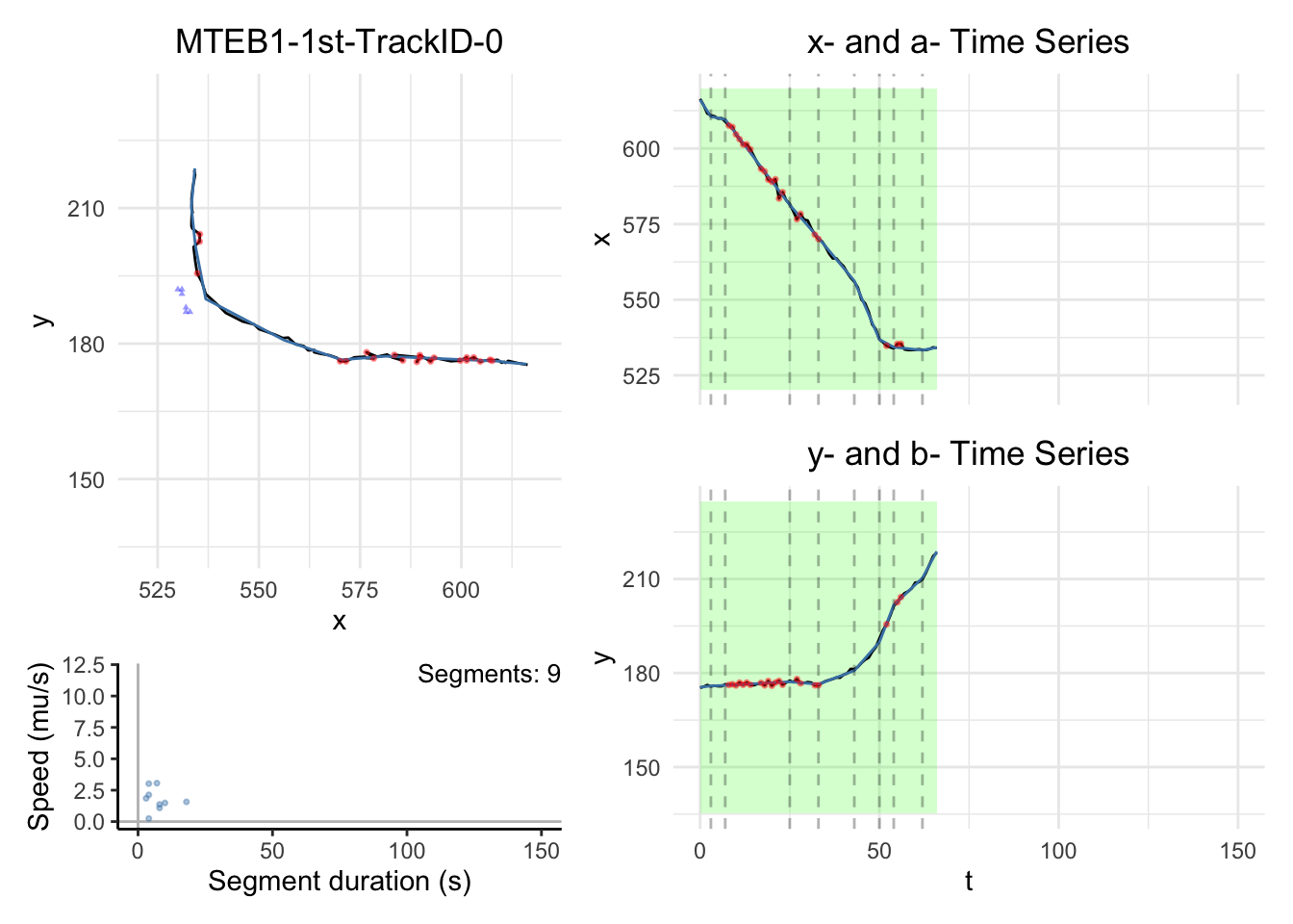
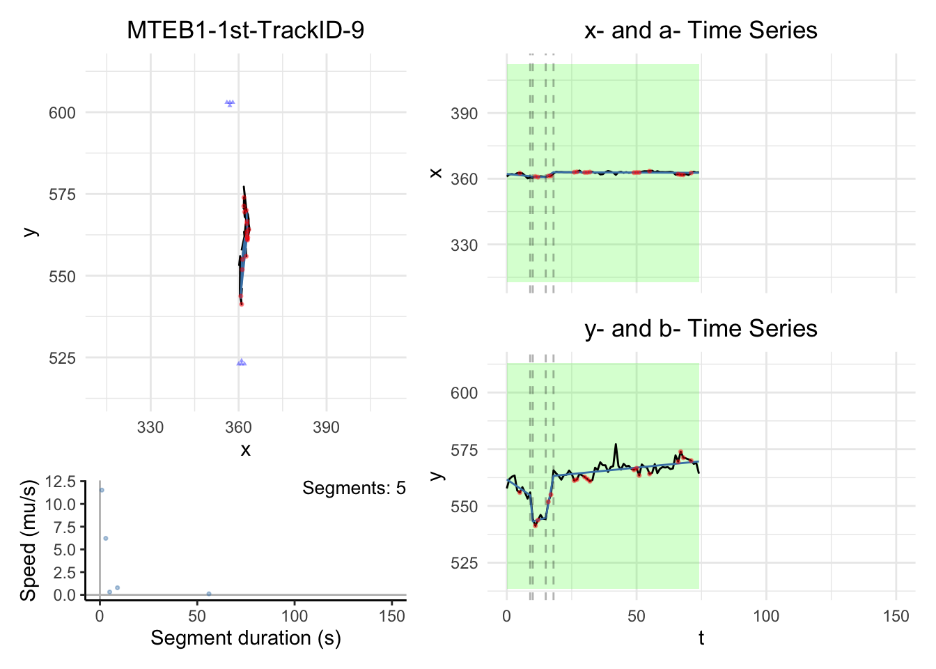
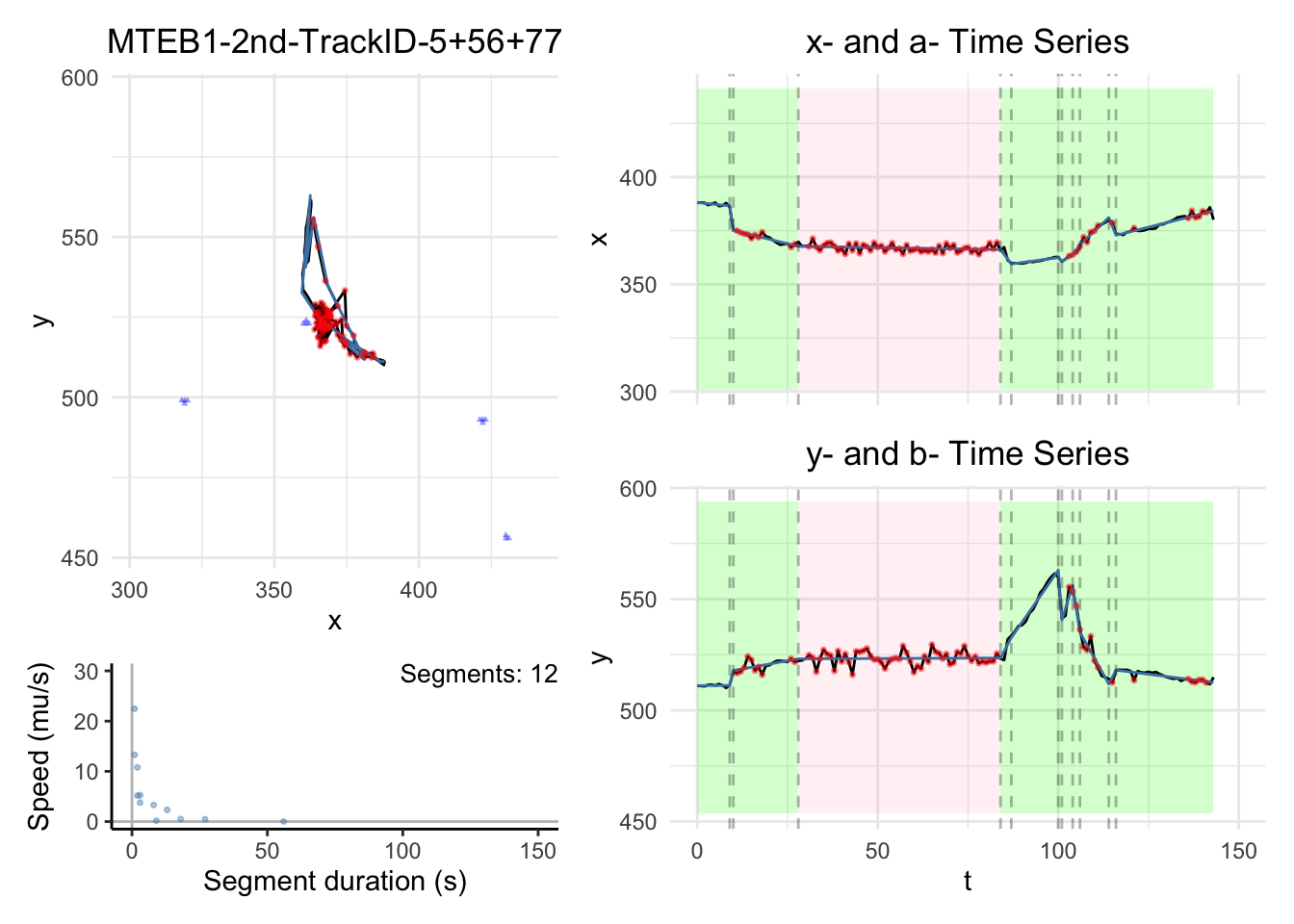
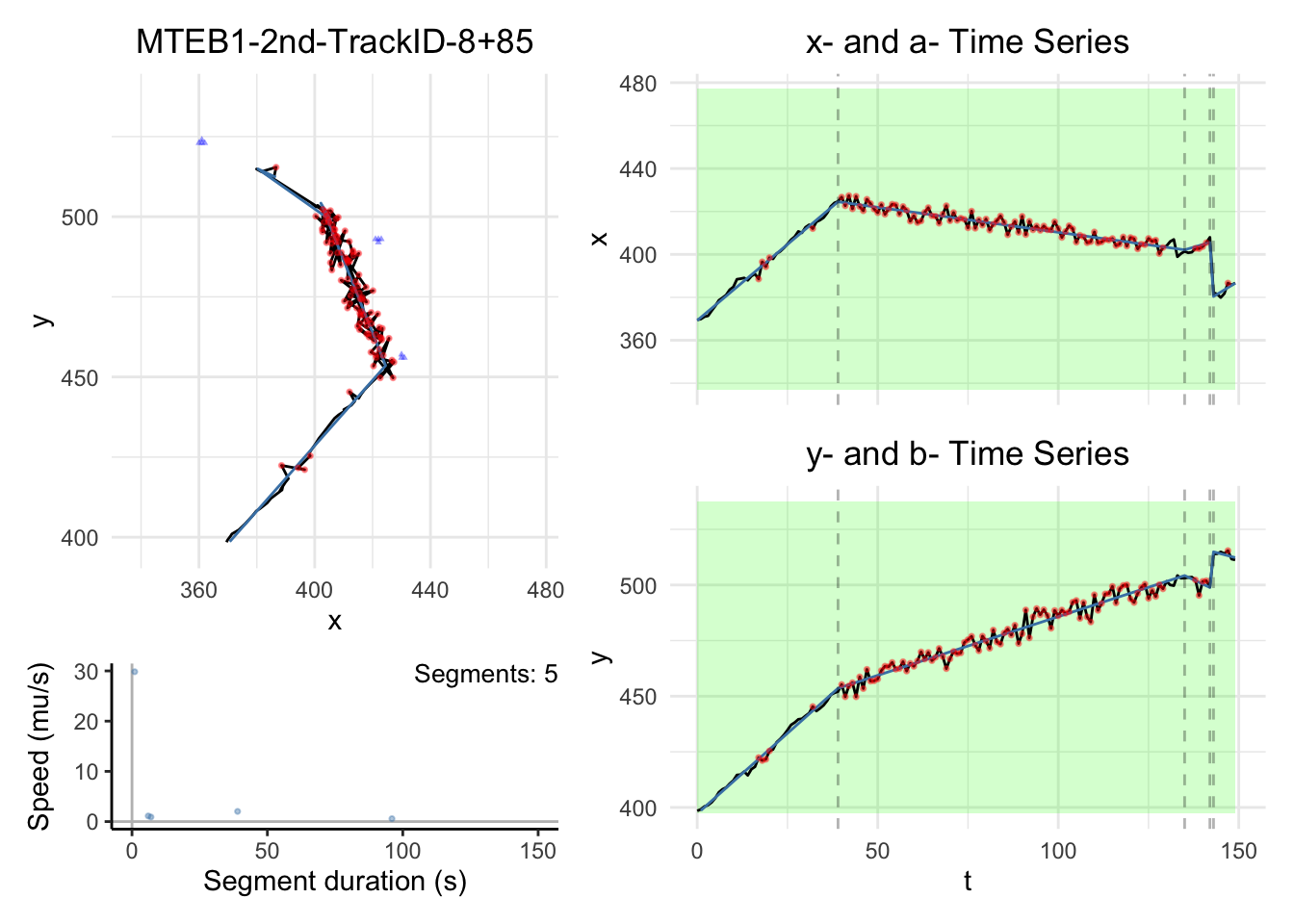
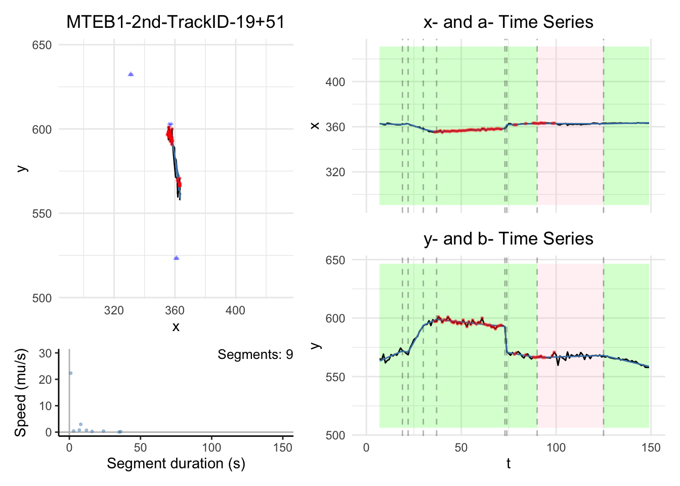
We will have some plots for the two tracks here. For the full gallary, please visit analysis/figures.

Note:

the black dashed-lines are for detected changepoint times.
The triangle blue dots are for the branch points.
The red dots are for the fill-in position.
The green areas show the motile segments while the pink areas show the stationary segments.

path_list = readRDS(here("data","CPLASS_MTEB1_1st.rds"))
#######################
motor = "MTEB1-1st" #change the name to the name of your data
dist_max = c()
t_max = c()
speed_max = c()

for (i in c(1,6)){
  path = path_list[[i]]$path_inferred
  segments = path_list[[i]]$segments_inferred
  speed_max = c(speed_max,max(path_list[[i]]$segments_inferred$speeds))
  
  dist_max = c(dist_max,max(c(max(path$x)-min(path$x)),
                            max((path$y)-min(path$y))))
  t_max = c(t_max,max(path$t) - min(path$t))
}
xy_width = 1.2*max(dist_max)
# t_lim = c(0,ceiling(max(t_max)))
t_lim = c(0,150)
max_speed = ceiling(max(speed_max))

for (i in c(1,6))
{
dashboard = plot_path_inferred_fill_in(path_list[[i]],xy_width,t_lim, motor, max_speed, branch_points = branch_points)
  print(dashboard)
}

Version	Author	Date
f71b1fa	Ldo3	2025-08-31

Version	Author	Date
f71b1fa	Ldo3	2025-08-31

# path_list = readRDS(here("data","CPLASS_MTEB1_1st.rds"))
# #######################
# # for REAL DATA use the lines below.
# file_list = c("MTEB1-1st")
# filestub = paste0("figures/Real",file_list[1])
# # infile = paste0(filestub,"_cplass.rds")
# outfile = paste0(filestub,"_gallery.pdf")
# # path_list = readRDS(infile)
# # 
# motor = "MTEB1-1st" #change the name to the name of your data
# 
# #######################
# # #for SIMULATED DATA use the lines below.
# # filestub = paste0("OFR Final/Sim",experiment_num,"_",theta$motor,"_",Hz,"Hz_cplass_",sp)
# # infile = paste0(filestub,".rds")
# # outfile = paste0(filestub,"_gallery_",sp,".pdf")
# # path_list = readRDS(infile)
# # 
# # if(theta$motor == "CKP"){
# #     motor = "Base"
# #   }else if(theta$motor == "kin1"){
# #     motor = "Contrast"
# #   }else if(theta$motor == "Mimic"){
# #     motor = "Mimic"
# # }
# 
# 
# pdf_output = TRUE
# 
# if (pdf_output == TRUE){
#   pdf(outfile,onefile = TRUE,width=7,height=5)
# }
# 
# dist_max = c()
# t_max = c()
# speed_max = c()
# 
# for (i in 1:length(path_list)){
#   if (i %% 20 == 0){
#     print(paste("Working on path",i))
#   }
#   path = path_list[[i]]$path_inferred
#   segments = path_list[[i]]$segments_inferred
#   speed_max = c(speed_max,max(path_list[[i]]$segments_inferred$speeds))
#   
#   dist_max = c(dist_max,max(c(max(path$x)-min(path$x)),
#                             max((path$y)-min(path$y))))
#   t_max = c(t_max,max(path$t) - min(path$t))
# }
# xy_width = 1.2*max(dist_max)
# # t_lim = c(0,ceiling(max(t_max)))
# t_lim = c(0,150)
# max_speed = ceiling(max(speed_max))
# 
# for (i in 1:length(path_list)){
#   if (i %% 20 == 0){
#     print(paste("Working on path",i))
#   }
#   
#   # #REAL DATA PLOTS (dashboard)
#   # dashboard = plot_path_real(path_list[[i]],xy_width,t_lim)
#   # print(dashboard)
# 
#   # SIMULATION PLOTS (dashboard)
#   dashboard = plot_path_inferred_fill_in(path_list[[i]],xy_width,t_lim, motor, max_speed, branch_points = branch_points)
#   print(dashboard)
# 
#   # SIMULATION PLOTS (only x-y plot)
#   # plot_xy = plot_path_inferred_xy(path_list[[i]],xy_width,t_lim, motor, max_speed)
#   # print(plot_xy)
#   
# }
# 
# if (pdf_output == TRUE){
#   dev.off()
# }

2. Second approach

A path \(j\) is considered as a potential candidate to merge to the \(i\)th-path if: \(t_{end}\) of \(i\)th-path \(< t_{start}\) of \(j\)th-path. For all potential candidates, calculate the Euclidean distance between the endpoint of path \(i\) and the start point of path \(j\), i.e., \[\sqrt{(x_{i_{end}}-x_{j_{start}})^2+(y_{i_{end}}-y_{j_{start}})^2}\] Among those candidates, select the one with the minimum distance value. Return the final candidate to merge. In the final round, we look at the video to confirm which case looks like a good merge.

With this strategy, we return 18 paths. The following shows the index of merged tracks corresponding to each path. For example, path 1 in this second approach is the output after merging TRACK 0 and TRACK 73.

oam = readRDS(here("data","original_tracks_after_merging.rds"))
chains = list()
for (i in 1:length(oam))
{
  chains[[i]] = unique(oam[[i]]$TRACK_ID)
}
# Build edges from consecutive nodes in each chain
edges <- do.call(rbind, lapply(chains, function(chain) {
  if (length(chain) > 1) {
    cbind(head(as.character(chain), -1),
          tail(as.character(chain), -1))
  } else NULL
}))

g <- graph_from_edgelist(edges, directed = TRUE)

plot(g,
     vertex.size = 17,
     vertex.label.cex = 1,
     vertex.color = "skyblue",
     edge.width = 2,            # make edges thicker
     edge.color = "darkred",    # change edge color
     edge.arrow.size = 1,     # make arrows bigger
     layout = layout_with_fr)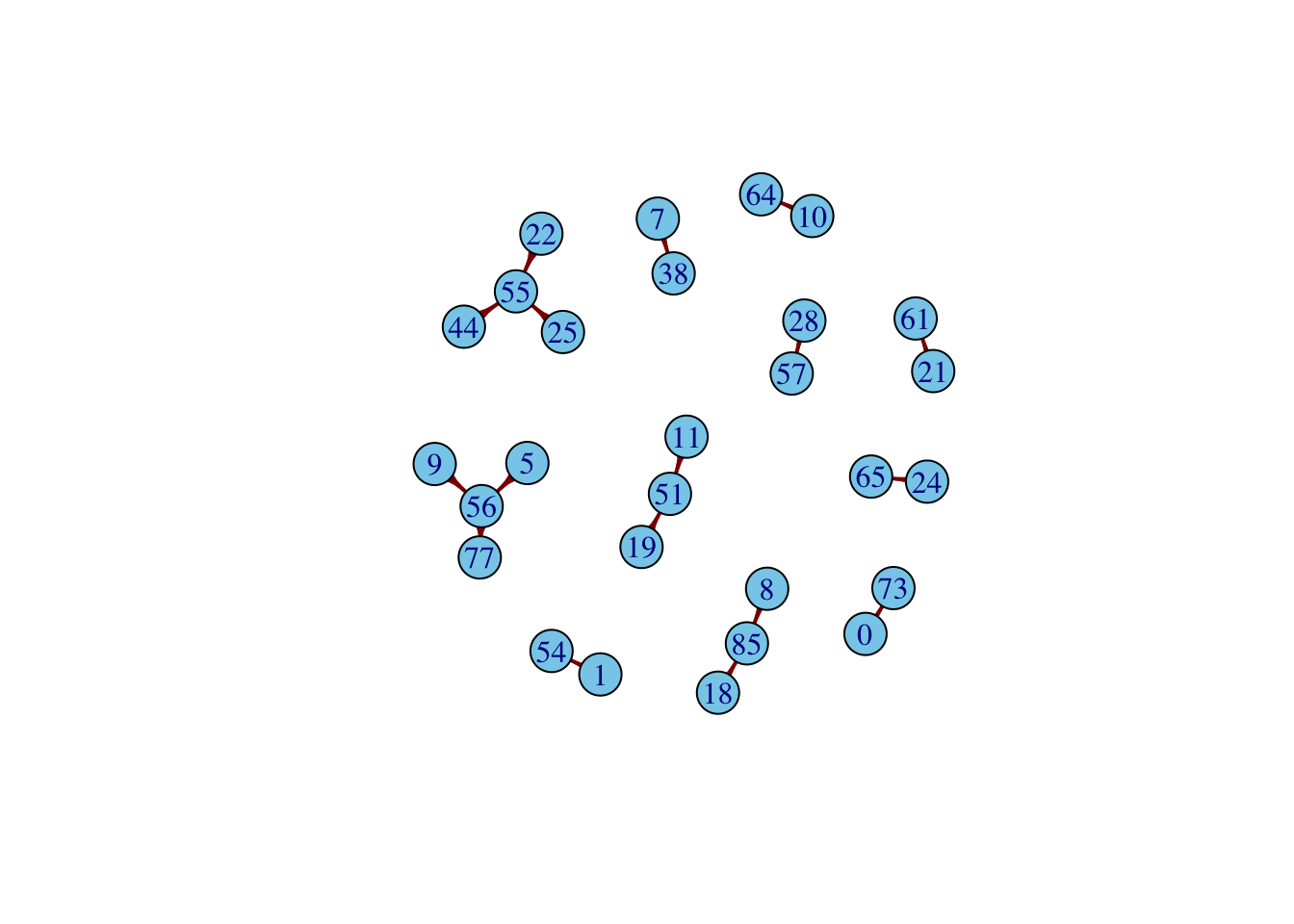

Version	Author	Date
f71b1fa	Ldo3	2025-08-31

There are missing time steps, we need to fill in those missing

af = list() #after fill-in
for (i in 1:length(oam))
{
  t = oam[[i]]$POSITION_T
  x = oam[[i]]$POSITION_X
  y = oam[[i]]$POSITION_Y
  track_id = unique(oam[[i]]$TRACK_ID)
  af[[i]] = fill_missing_data(t,x,y,track_id = track_id)
}
# saveRDS(af,here("data","second_approach_data.rds"))

2.1. Run CPLASS

# cplass_paths = CPLASS_paths(af, time_rate = 1,iter_max = 4000, PARALLEL = FALSE, speed_pen = FALSE)
# saveRDS(cplass_paths,file="data/CPLASS_MTEB1_2nd.rds")

2.2. Visualization

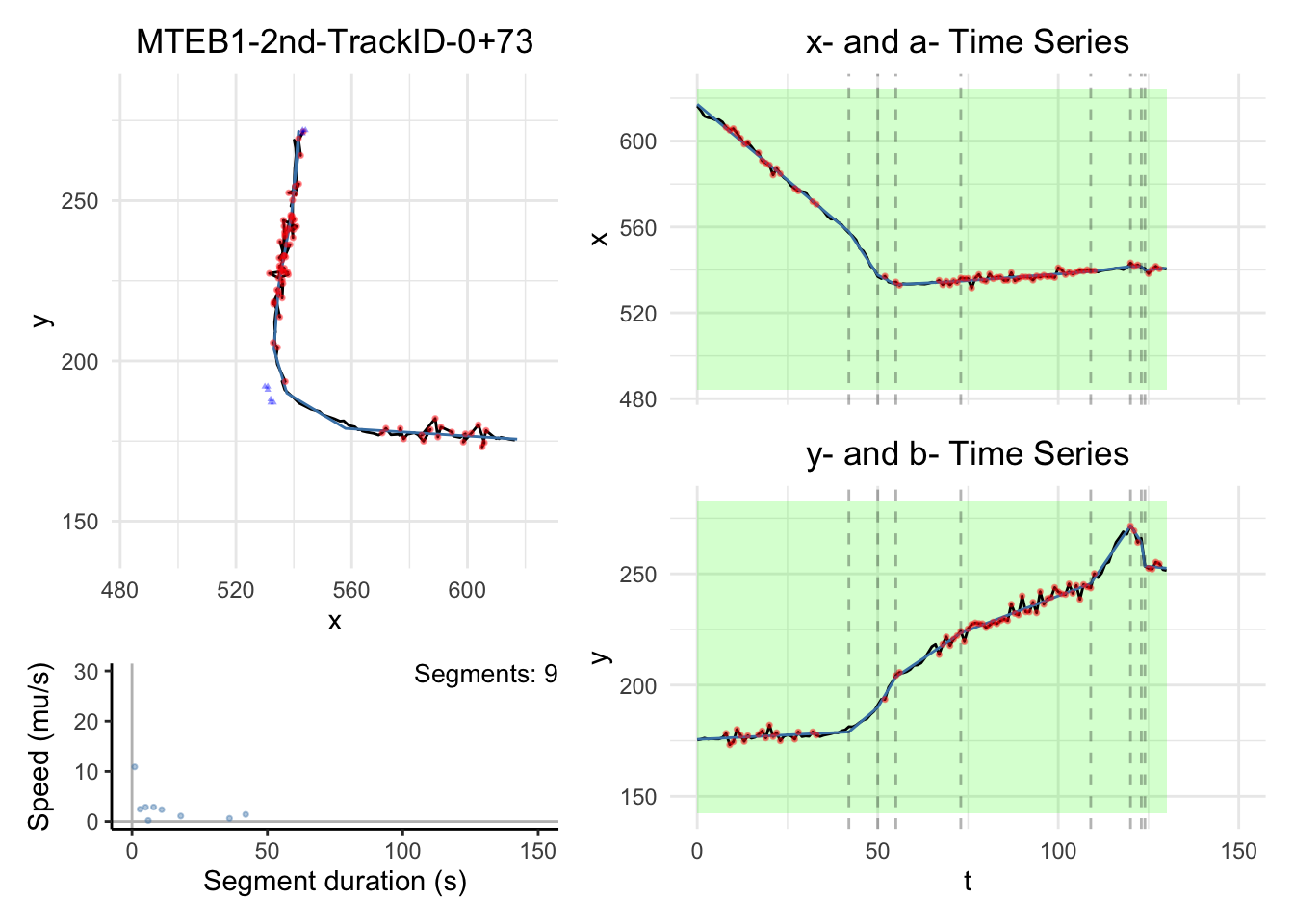
We will have some plots for some tracks here. For the full gallary, please visit analysis/figures.

Note:

the black dashed-lines are for detected changepoint times.
The triangle blue dots are for the branch points.
The red dots are for the fill-in position.
The green areas show the motile segments while the pink areas show the stationary segments.

path_list = readRDS(here("data","CPLASS_MTEB1_2nd.rds"))
#######################
# for REAL DATA use the lines below.
file_list = c("MTEB1-2nd")
filestub = paste0("figures/Real",file_list[1])
# infile = paste0(filestub,"_cplass.rds")
outfile = paste0(filestub,"_gallery.pdf")
# path_list = readRDS(infile)
# 
motor = "MTEB1-2nd" #change the name to the name of your data
dist_max = c()
t_max = c()
speed_max = c()

for (i in c(1,3,5,10)){
  path = path_list[[i]]$path_inferred
  segments = path_list[[i]]$segments_inferred
  speed_max = c(speed_max,max(path_list[[i]]$segments_inferred$speeds))
  
  dist_max = c(dist_max,max(c(max(path$x)-min(path$x)),
                            max((path$y)-min(path$y))))
  t_max = c(t_max,max(path$t) - min(path$t))
}
xy_width = 1.2*max(dist_max)
# t_lim = c(0,ceiling(max(t_max)))
t_lim = c(0,150)
max_speed = ceiling(max(speed_max))

for (i in c(1,3,5,10))
{
dashboard = plot_path_inferred_fill_in(path_list[[i]],xy_width,t_lim, motor, max_speed, branch_points = branch_points)
  print(dashboard)
}

Version	Author	Date
f71b1fa	Ldo3	2025-08-31

Version	Author	Date
f71b1fa	Ldo3	2025-08-31

Version	Author	Date
f71b1fa	Ldo3	2025-08-31

Version	Author	Date
f71b1fa	Ldo3	2025-08-31

# path_list = readRDS(here("data","CPLASS_MTEB1_2nd.rds"))
# #######################
# # for REAL DATA use the lines below.
# file_list = c("MTEB1-2nd")
# filestub = paste0("figures/Real",file_list[1])
# # infile = paste0(filestub,"_cplass.rds")
# outfile = paste0(filestub,"_gallery.pdf")
# # path_list = readRDS(infile)
# # 
# motor = "MTEB1-2nd" #change the name to the name of your data
# 
# #######################
# # #for SIMULATED DATA use the lines below.
# # filestub = paste0("OFR Final/Sim",experiment_num,"_",theta$motor,"_",Hz,"Hz_cplass_",sp)
# # infile = paste0(filestub,".rds")
# # outfile = paste0(filestub,"_gallery_",sp,".pdf")
# # path_list = readRDS(infile)
# # 
# # if(theta$motor == "CKP"){
# #     motor = "Base"
# #   }else if(theta$motor == "kin1"){
# #     motor = "Contrast"
# #   }else if(theta$motor == "Mimic"){
# #     motor = "Mimic"
# # }
# 
# 
# pdf_output = TRUE
# 
# if (pdf_output == TRUE){
#   pdf(outfile,onefile = TRUE,width=7,height=5)
# }
# 
# dist_max = c()
# t_max = c()
# speed_max = c()
# 
# for (i in 1:length(path_list)){
#   if (i %% 20 == 0){
#     print(paste("Working on path",i))
#   }
#   path = path_list[[i]]$path_inferred
#   segments = path_list[[i]]$segments_inferred
#   speed_max = c(speed_max,max(path_list[[i]]$segments_inferred$speeds))
#   
#   dist_max = c(dist_max,max(c(max(path$x)-min(path$x)),
#                             max((path$y)-min(path$y))))
#   t_max = c(t_max,max(path$t) - min(path$t))
# }
# xy_width = 1.2*max(dist_max)
# # t_lim = c(0,ceiling(max(t_max)))
# t_lim = c(0,150)
# max_speed = ceiling(max(speed_max))
# 
# for (i in 1:length(path_list)){
#   if (i %% 20 == 0){
#     print(paste("Working on path",i))
#   }
#   
#   # #REAL DATA PLOTS (dashboard)
#   # dashboard = plot_path_real(path_list[[i]],xy_width,t_lim)
#   # print(dashboard)
# 
#   # SIMULATION PLOTS (dashboard)
#   dashboard = plot_path_inferred_fill_in(path_list[[i]],xy_width,t_lim, motor, max_speed, branch_points = branch_points)
#   print(dashboard)
# 
#   # SIMULATION PLOTS (only x-y plot)
#   # plot_xy = plot_path_inferred_xy(path_list[[i]],xy_width,t_lim, motor, max_speed)
#   # print(plot_xy)
#   
# }
# 
# if (pdf_output == TRUE){
#   dev.off()
# }

Run CSA for both approaches

pdf_output = TRUE

real_data_not_merged_file = c(here("data","CPLASS_MTEB1_1st.rds"))
real_data_merged_file = c(here("data","CPLASS_MTEB1_2nd.rds"))

real_path_not_merged_list = readRDS(real_data_not_merged_file)
real_path_merged_list = readRDS(real_data_merged_file)


cohort_list = c("MTEB1: 1st approach", 
                "MTEB1: 2nd approach")
color_list = c("MTEB1: 1st approach" = "grey", 
               "MTEB1: 2nd approach" = "lightblue") 

pdf_output = TRUE


##### Create Segment Summary ####
segment_summary = summarize_segments_inferred(real_path_not_merged_list,cohort_list[1])
segment_summary = bind_rows(segment_summary,
                            summarize_segments(real_path_merged_list,cohort_list[2]))

max_speed = min(15,max(segment_summary$speeds))

# Assumes theta is the same for all frame rates involved
speed_mesh = seq(0,max_speed,length = 200)
ds = speed_mesh[2] - speed_mesh[1]
subsample_size = 200
num_subsamples = 30

csa = tibble()
#### Bootstrap CSA for Real Data 1st approach ####
for (m in 1:num_subsamples){
    subsample = sample(1:length(real_path_not_merged_list),subsample_size,replace = TRUE)
    path_subsample = list()
    for (i in 1:length(subsample)){
      path_subsample[[i]] = real_path_not_merged_list[[subsample[i]]]
    }
    this_segments_summary = summarize_segments_inferred(path_subsample,"Sample")
    this_csa = compute_csa(this_segments_summary, speed_mesh)$csa
    csa = bind_rows(csa,
                tibble(
                  s = speed_mesh,
                  csa = this_csa,
                  dcsa = c(diff(this_csa)/ds,0),
                  error = NA,
                  error_pct = NA,
                  label = cohort_list[1],
                  Hz = NA,
                  subsample = m
                ))
}


#### Bootstrap CSA for Real Data 2nd approach ####
for (m in 1:num_subsamples){
    subsample = sample(1:length(real_path_merged_list),subsample_size,replace = TRUE)
    path_subsample = list()
    for (i in 1:length(subsample)){
      path_subsample[[i]] = real_path_merged_list[[subsample[i]]]
    }
    this_segments_summary = summarize_segments_inferred(path_subsample,"Sample")
    this_csa = compute_csa(this_segments_summary, speed_mesh)$csa
    csa = bind_rows(csa,
                tibble(
                  s = speed_mesh,
                  csa = this_csa,
                  dcsa = c(diff(this_csa)/ds,0),
                  error = NA,
                  error_pct = NA,
                  label = cohort_list[2],
                  Hz = NA,
                  subsample = m
                ))
}


csa = csa %>% mutate(cohort = paste(label,subsample))


p_csa = ggplot(csa %>% filter(label == cohort_list[1] | 
                                      label == cohort_list[2]))+
  geom_line(aes(x = s, y = csa, col = label, group = cohort))+
  ggtitle("MTEB1")+
  ylab("Cumulative Speed Allocation")+xlab(expression(paste("Speed (",mu,"m/sec)")))+
  scale_color_manual(values = color_list)+
  theme_minimal()
# +
  # theme(legend.position = "none")

print(p_csa)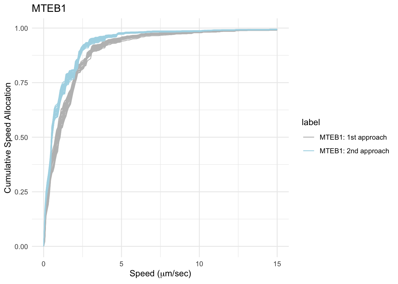

Version	Author	Date
f71b1fa	Ldo3	2025-08-31

speed_df1 = segment_summary%>% filter(label=="MTEB1: 1st approach")
speed_df2 = segment_summary%>% filter(label=="MTEB1: 2nd approach")

print("The highest speed value in the first approach is")

[1] "The highest speed value in the first approach is"

speed_df1%>% filter(speeds ==max(speeds))

# A tibble: 1 × 5
  durations states speeds label               path_id
      <dbl>  <dbl>  <dbl> <chr>                 <int>
1         1      1   28.4 MTEB1: 1st approach      34

print("The highest speed value in the second approach is")

[1] "The highest speed value in the second approach is"

speed_df2%>% filter(speeds ==max(speeds))

# A tibble: 1 × 5
  durations states speeds label               path_id
      <dbl>  <dbl>  <dbl> <chr>                 <int>
1         1      1   30.8 MTEB1: 2nd approach       9

ggplot(segment_summary, aes(x = speeds, fill = label)) +
  geom_density(alpha = 0.4) +
  labs(title = "KDE of inferred speed in different approaches", x = "Speed (mu/s)", y = "Density") +
  theme_minimal()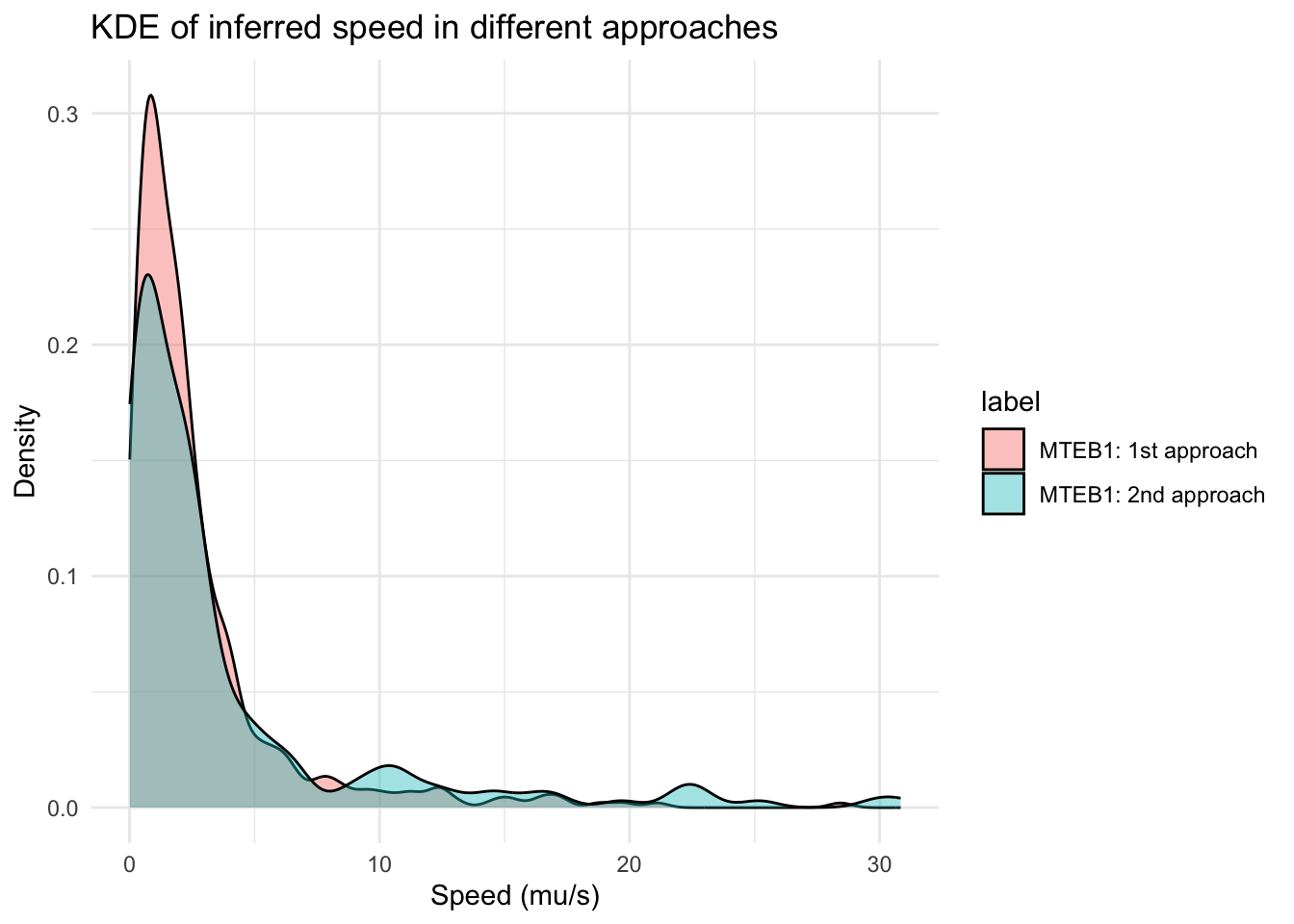

Version	Author	Date
f71b1fa	Ldo3	2025-08-31

From the CSA plot, the second approach provide more segments will speed between 0 -5 \(\mu m/s\) than in the first approach.

Merged tracks in the second approach provide us clearer picture where a blob pass branch points, e.g., paths we plotted above.

We also want to point out that CPLASS does not work well with too short path such as 10-20 time steps (see the plot gallery for the first approach), i.e., for too short path, the algorithm will detect a lot of changepoints. In the CPLASS, we discussed the consistency theory of CPLASS when we have the sample size is large enough.

sessionInfo()

R version 4.5.1 (2025-06-13)
Platform: aarch64-apple-darwin20
Running under: macOS Ventura 13.1

Matrix products: default
BLAS:   /Library/Frameworks/R.framework/Versions/4.5-arm64/Resources/lib/libRblas.0.dylib 
LAPACK: /Library/Frameworks/R.framework/Versions/4.5-arm64/Resources/lib/libRlapack.dylib;  LAPACK version 3.12.1

locale:
[1] en_US.UTF-8/en_US.UTF-8/en_US.UTF-8/C/en_US.UTF-8/en_US.UTF-8

time zone: America/Chicago
tzcode source: internal

attached base packages:
[1] parallel  stats     graphics  grDevices utils     datasets  methods  
[8] base     

other attached packages:
 [1] igraph_2.1.4      doParallel_1.0.17 iterators_1.0.14  foreach_1.5.2    
 [5] patchwork_1.3.2   lubridate_1.9.4   forcats_1.0.0     stringr_1.5.1    
 [9] dplyr_1.1.4       purrr_1.1.0       readr_2.1.5       tidyr_1.3.1      
[13] tibble_3.3.0      ggplot2_3.5.2     tidyverse_2.0.0   limSolve_2.0.1   
[17] pracma_2.4.4      matrixcalc_1.0-6  Rlab_4.0          here_1.0.1       

loaded via a namespace (and not attached):
 [1] gtable_0.3.6       xfun_0.53          bslib_0.9.0        tzdb_0.5.0        
 [5] quadprog_1.5-8     vctrs_0.6.5        tools_4.5.1        generics_0.1.4    
 [9] pkgconfig_2.0.3    RColorBrewer_1.1-3 lifecycle_1.0.4    compiler_4.5.1    
[13] farver_2.1.2       git2r_0.36.2       codetools_0.2-20   httpuv_1.6.16     
[17] htmltools_0.5.8.1  sass_0.4.10        yaml_2.3.10        crayon_1.5.3      
[21] later_1.4.3        pillar_1.11.0      jquerylib_0.1.4    whisker_0.4.1     
[25] MASS_7.3-65        cachem_1.1.0       tidyselect_1.2.1   digest_0.6.37     
[29] stringi_1.8.7      labeling_0.4.3     rprojroot_2.1.1    fastmap_1.2.0     
[33] grid_4.5.1         cli_3.6.5          magrittr_2.0.3     utf8_1.2.6        
[37] withr_3.0.2        scales_1.4.0       promises_1.3.3     bit64_4.6.0-1     
[41] timechange_0.3.0   rmarkdown_2.29     bit_4.6.0          workflowr_1.7.2   
[45] hms_1.1.3          evaluate_1.0.4     lpSolve_5.6.23     knitr_1.50        
[49] rlang_1.1.6        Rcpp_1.1.0         glue_1.8.0         rstudioapi_0.17.1 
[53] vroom_1.6.5        jsonlite_2.0.0     R6_2.6.1           fs_1.6.6