E18 mLN pLN EYFP+
A.DeMartin
2025-05-23
Last updated: 2025-07-15
Checks: 6 1
Knit directory: LNdevMouse24.2/
This reproducible R Markdown analysis was created with workflowr (version 1.7.1). The Checks tab describes the reproducibility checks that were applied when the results were created. The Past versions tab lists the development history.
The R Markdown is untracked by Git. To know which version of the R
Markdown file created these results, you’ll want to first commit it to
the Git repo. If you’re still working on the analysis, you can ignore
this warning. When you’re finished, you can run
wflow_publish to commit the R Markdown file and build the
HTML.
Great job! The global environment was empty. Objects defined in the global environment can affect the analysis in your R Markdown file in unknown ways. For reproduciblity it’s best to always run the code in an empty environment.
The command set.seed(20250625) was run prior to running
the code in the R Markdown file. Setting a seed ensures that any results
that rely on randomness, e.g. subsampling or permutations, are
reproducible.
Great job! Recording the operating system, R version, and package versions is critical for reproducibility.
Nice! There were no cached chunks for this analysis, so you can be confident that you successfully produced the results during this run.
Great job! Using relative paths to the files within your workflowr project makes it easier to run your code on other machines.
Great! You are using Git for version control. Tracking code development and connecting the code version to the results is critical for reproducibility.
The results in this page were generated with repository version a9ff376. See the Past versions tab to see a history of the changes made to the R Markdown and HTML files.
Note that you need to be careful to ensure that all relevant files for
the analysis have been committed to Git prior to generating the results
(you can use wflow_publish or
wflow_git_commit). workflowr only checks the R Markdown
file, but you know if there are other scripts or data files that it
depends on. Below is the status of the Git repository when the results
were generated:
Ignored files:
    Ignored:    .DS_Store
    Ignored:    .Rhistory
    Ignored:    .Rproj.user/
    Ignored:    analysis/.DS_Store
    Ignored:    data/to figshare/
    Ignored:    data/tradeSEQ/

Untracked files:
    Untracked:  analysis/E18_mLN_iLN_EYFPonly_marker.Rmd

Unstaged changes:
    Modified:   analysis/index.Rmd
Note that any generated files, e.g. HTML, png, CSS, etc., are not included in this status report because it is ok for generated content to have uncommitted changes.
There are no past versions. Publish this analysis with
wflow_publish() to start tracking its development.
reprocess
load packages
set color vectors
coltimepoint <- c("#440154FF", "#3B528BFF", "#21908CFF", "#5DC863FF")
names(coltimepoint) <- c("E18", "P7", "3w", "8w")

collocation <- c("#61baba", "#ba6161")
names(collocation) <- c("iLN", "mLN")
load object all
basedir <- here()
fileNam <- paste0(basedir, "/data/LNmLToRev_allmerged_seurat.rds")
seuratM <- readRDS(fileNam)
table(seuratM$timepoint)
  E18    P7    3w    8w
42711 44836 29577 23167
table(seuratM$orig.ident)
140291 subset E18
seuratA <- subset(seuratM, timepoint == "E18")
table(seuratA$timepoint)
  E18
42711
seuratA <- JoinLayers(seuratA)
#rerun seurat
seuratA <- NormalizeData (object = seuratA)
seuratA <- FindVariableFeatures(object = seuratA)
seuratA <- ScaleData(object = seuratA, verbose = TRUE)
seuratA <- RunPCA(object=seuratA, npcs = 30, verbose = FALSE)
seuratA <- RunTSNE(object=seuratA, reduction="pca", dims = 1:20)
seuratA <- RunUMAP(object=seuratA, reduction="pca", dims = 1:20)
seuratA <- FindNeighbors(object = seuratA, reduction = "pca", dims= 1:20)
res <- c(0.25, 0.6, 0.8, 0.4)
for (i in 1:length(res)) {
seuratA <- FindClusters(object = seuratA, resolution = res[i], random.seed = 1234)
}Modularity Optimizer version 1.3.0 by Ludo Waltman and Nees Jan van Eck
Number of nodes: 42711
Number of edges: 1412581
Running Louvain algorithm...
Maximum modularity in 10 random starts: 0.9485
Number of communities: 15
Elapsed time: 7 seconds
Modularity Optimizer version 1.3.0 by Ludo Waltman and Nees Jan van Eck
Number of nodes: 42711
Number of edges: 1412581
Running Louvain algorithm...
Maximum modularity in 10 random starts: 0.9170
Number of communities: 21
Elapsed time: 9 seconds
Modularity Optimizer version 1.3.0 by Ludo Waltman and Nees Jan van Eck
Number of nodes: 42711
Number of edges: 1412581
Running Louvain algorithm...
Maximum modularity in 10 random starts: 0.9042
Number of communities: 25
Elapsed time: 9 seconds
Modularity Optimizer version 1.3.0 by Ludo Waltman and Nees Jan van Eck
Number of nodes: 42711
Number of edges: 1412581
Running Louvain algorithm...
Maximum modularity in 10 random starts: 0.9329
Number of communities: 17
Elapsed time: 8 secondsdimplot all
clustering
Idents(seuratA) <- seuratA$RNA_snn_res.0.25
DimPlot(seuratA, reduction = "umap", group.by = "RNA_snn_res.0.25" ,
        pt.size = 0.1, label = T, shuffle = T) +
  theme_bw() +
  theme(axis.text = element_blank(), axis.ticks = element_blank(),
        panel.grid.minor = element_blank()) +
  xlab("umap1") +
  ylab("umap2")
location
DimPlot(seuratA, reduction = "umap", group.by = "location" ,
pt.size = 0.1, label = T, shuffle = T) +
theme_bw() +
theme(axis.text = element_blank(), axis.ticks = element_blank(),
panel.grid.minor = element_blank()) +
xlab("umap1") +
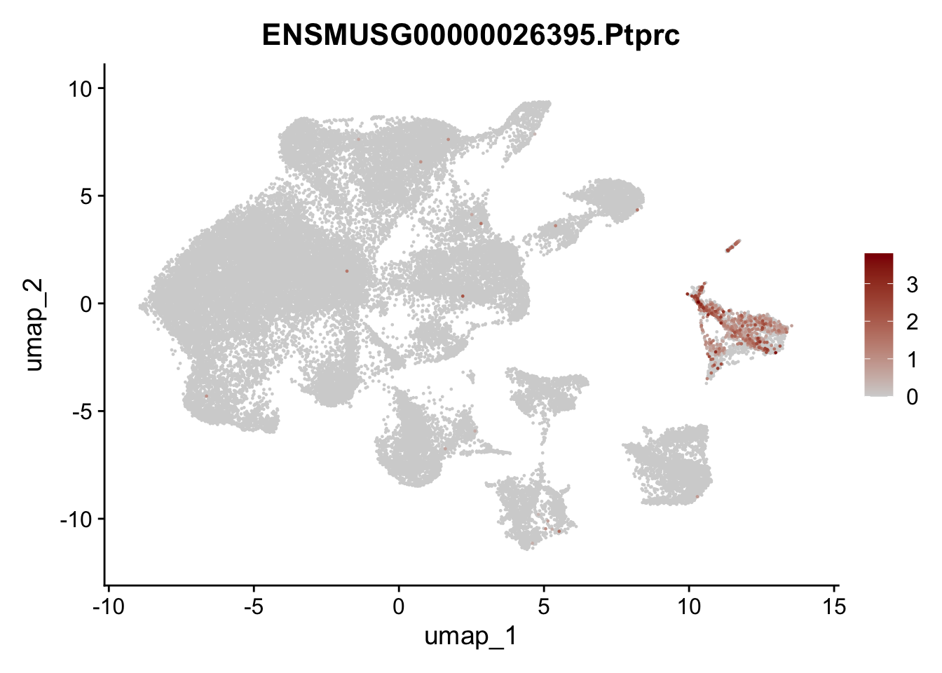
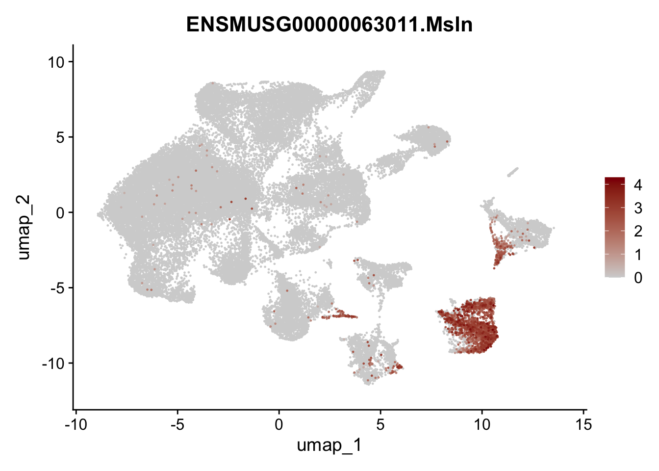
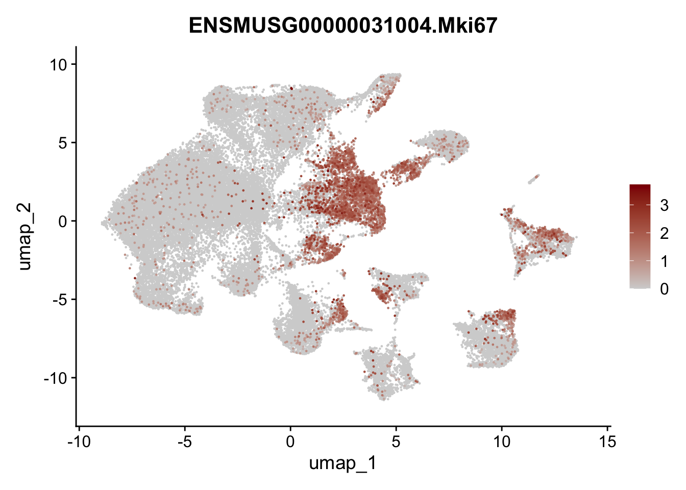
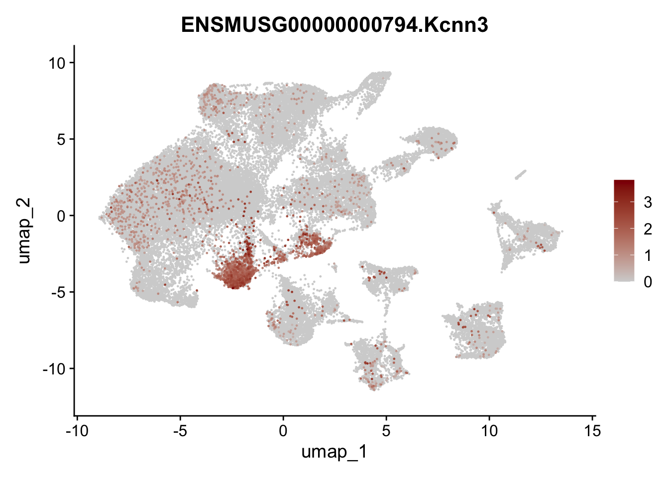
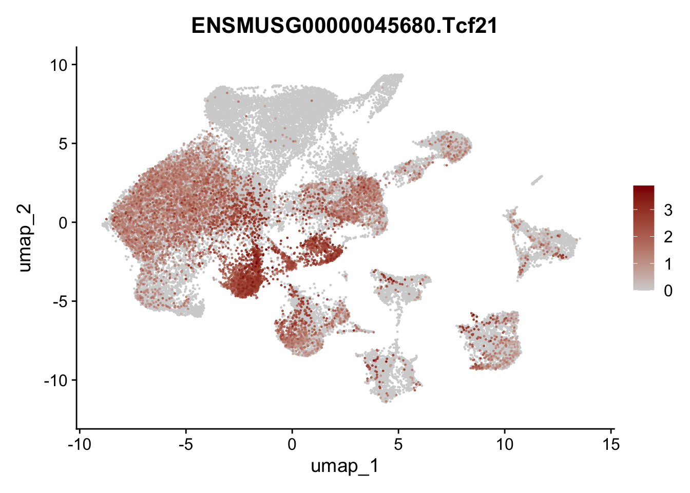
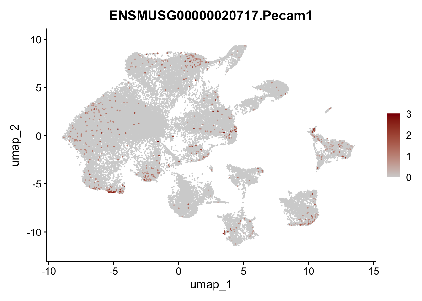
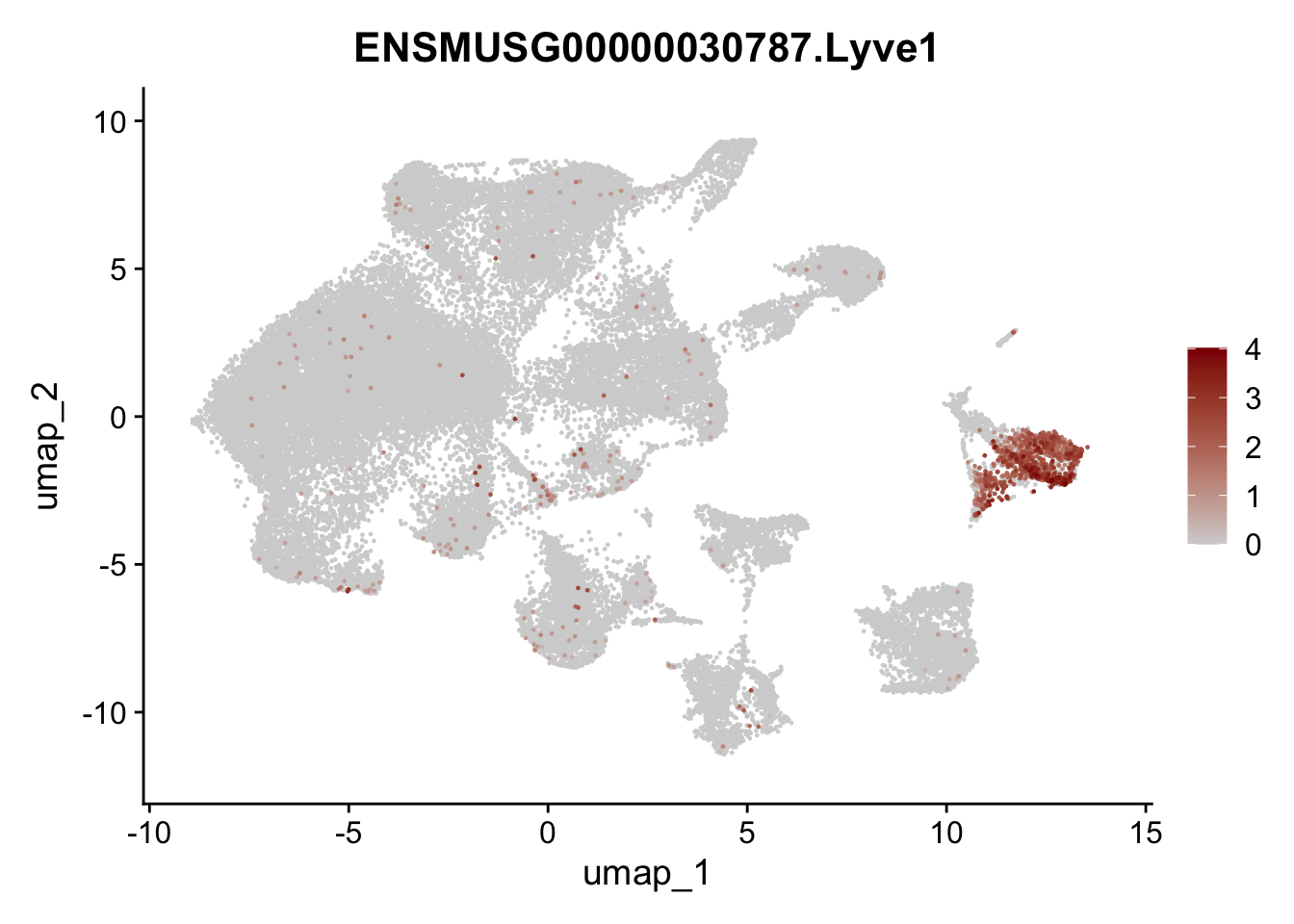
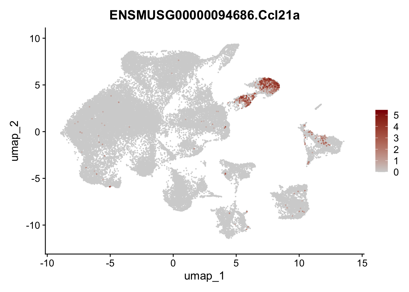
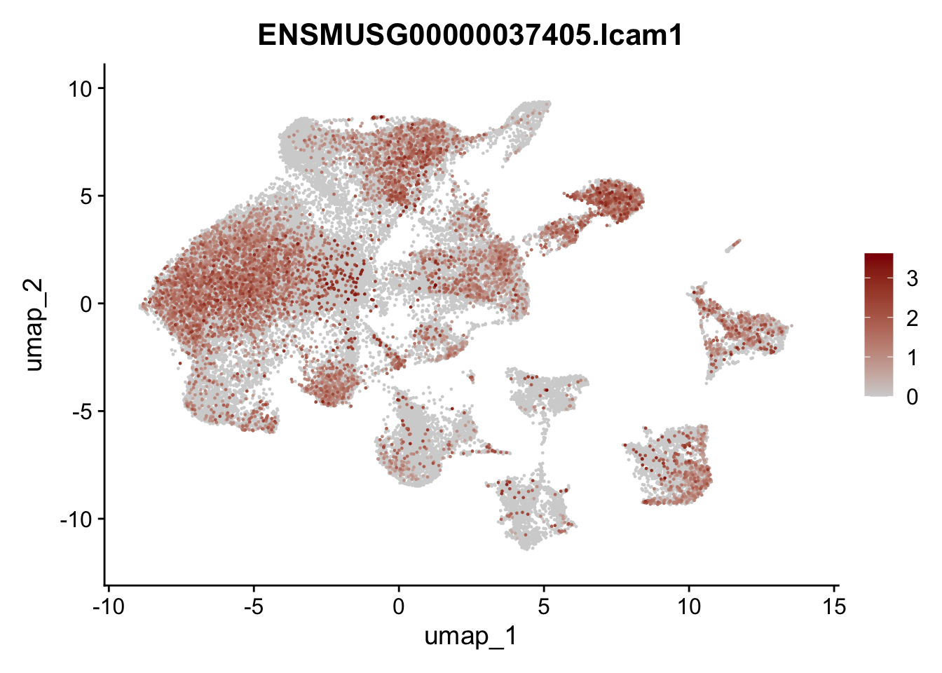
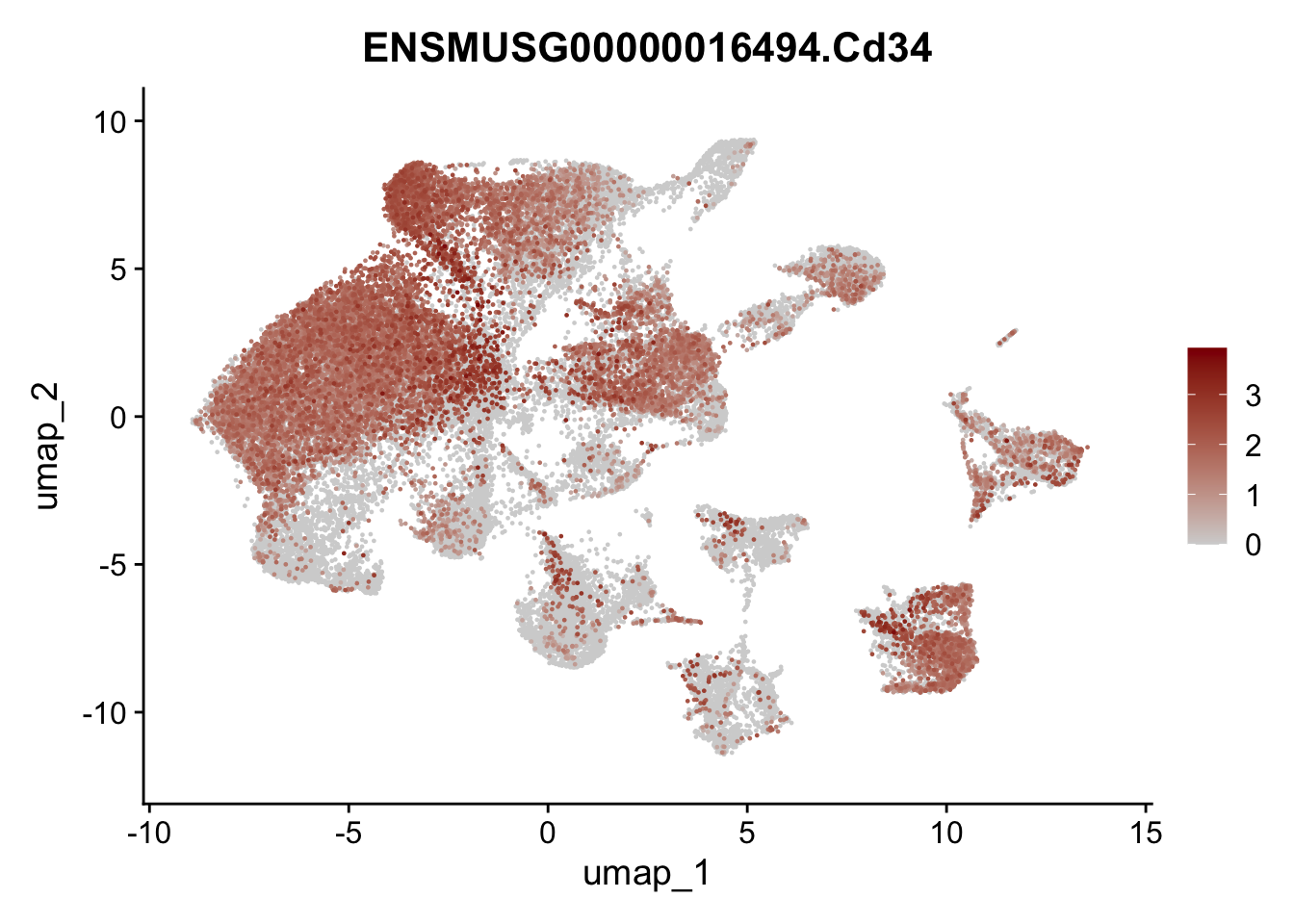
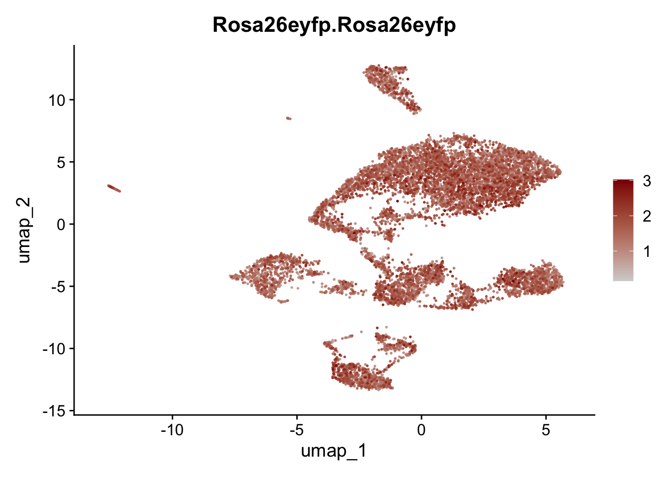
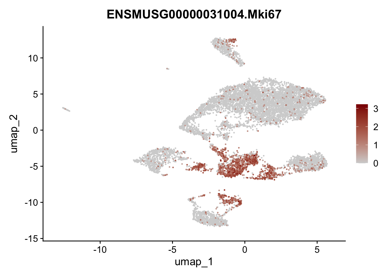
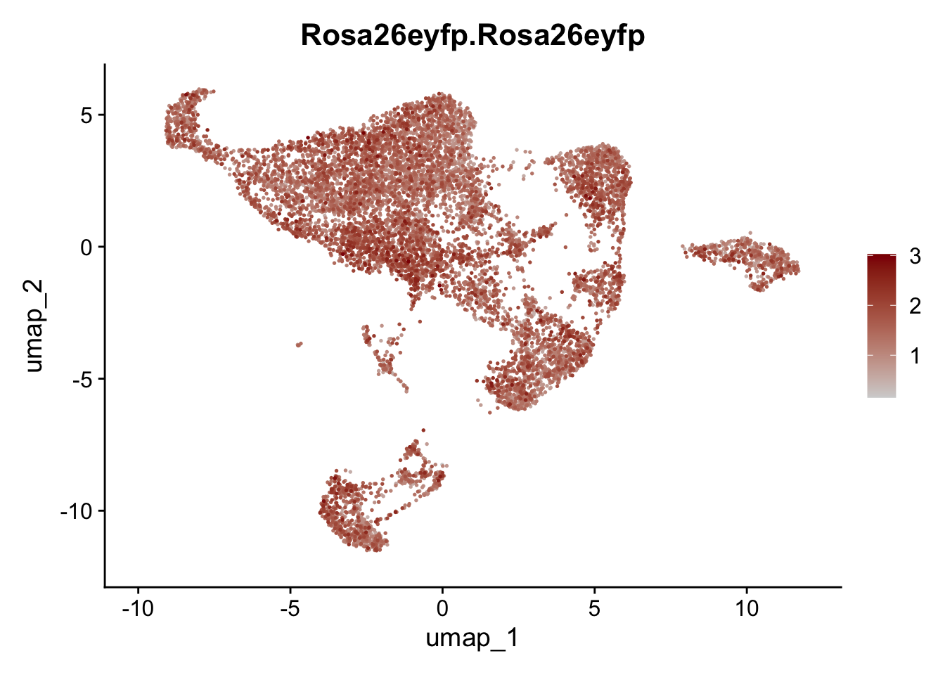
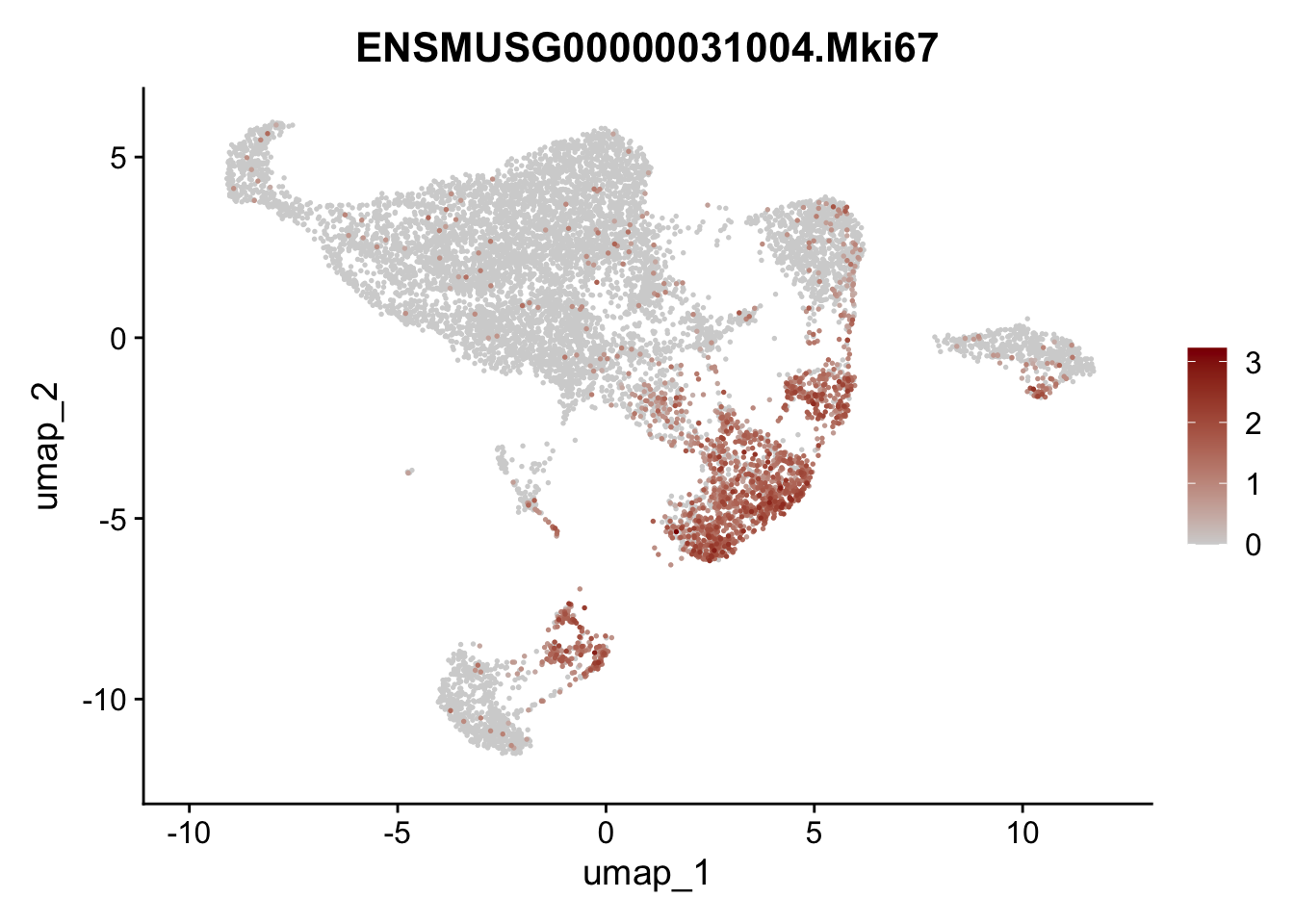
ylab("umap2")features
genes <- data.frame(gene=rownames(seuratA)) %>%
    mutate(geneID=gsub("^.*\\.", "", gene))

selGenes <- data.frame(geneID=c("Ptprc", "Msln", "Mki67", "Kcnn3", "Tcf21", "Pecam1", "Lyve1", "Ccl21a", "Icam1", "Cd34")) %>%
  left_join(., genes, by = "geneID")

pList <- sapply(selGenes$gene, function(x){
  p <- FeaturePlot(seuratA, reduction = "umap",
            features = x,
            cols=c("lightgrey","darkred"),
            order = T)+
  theme(legend.position="right")
  plot(p)
})
filter
## filter Ptprc+ cells (cluster #7 and #14)
table(seuratA$RNA_snn_res.0.25)
seuratF <- subset(seuratA, RNA_snn_res.0.25 %in% c("7", "14"), invert = TRUE)
table(seuratF$RNA_snn_res.0.25)

seuratE18fil <- seuratF
remove(seuratF)
rerun after fil
#rerun seurat
seuratE18fil <- NormalizeData (object = seuratE18fil)
seuratE18fil <- FindVariableFeatures(object = seuratE18fil)
seuratE18fil <- ScaleData(object = seuratE18fil, verbose = TRUE)
seuratE18fil <- RunPCA(object=seuratE18fil, npcs = 30, verbose = FALSE)
seuratE18fil <- RunTSNE(object=seuratE18fil, reduction="pca", dims = 1:20)
seuratE18fil <- RunUMAP(object=seuratE18fil, reduction="pca", dims = 1:20)
seuratE18fil <- FindNeighbors(object = seuratE18fil, reduction = "pca", dims= 1:20)

res <- c(0.25, 0.6, 0.8, 0.4)
for (i in 1:length(res)) {
  seuratE18fil <- FindClusters(object = seuratE18fil, resolution = res[i], random.seed = 1234)
}
load object fil
fileNam <- paste0(basedir, "/data/LNmLToRev_E18fil_seurat.rds")
seuratE18fil <- readRDS(fileNam)
dimplot E18 fil
clustering
Idents(seuratE18fil) <- seuratE18fil$RNA_snn_res.0.25
colPal <- c("#DAF7A6", "#FFC300", "#FF5733", "#C70039", "#900C3F", "#b66e8d",
            "#61a4ba", "#6178ba", "#54a87f",  "#25328a",
            "#b6856e", "#0073C2FF", "#EFC000FF", "#868686FF", "#CD534CFF",
            "#7AA6DCFF", "#003C67FF", "#8F7700FF", "#3B3B3BFF", "#A73030FF",
            "#4A6990FF")[1:length(unique(seuratE18fil$RNA_snn_res.0.25))]
names(colPal) <- unique(seuratE18fil$RNA_snn_res.0.25)

DimPlot(seuratE18fil, reduction = "umap", group.by = "RNA_snn_res.0.25",
        cols = colPal, label = TRUE)+
  theme_bw() +
  theme(axis.text = element_blank(), axis.ticks = element_blank(),
        panel.grid.minor = element_blank()) +
  xlab("UMAP1") +
  ylab("UMAP2")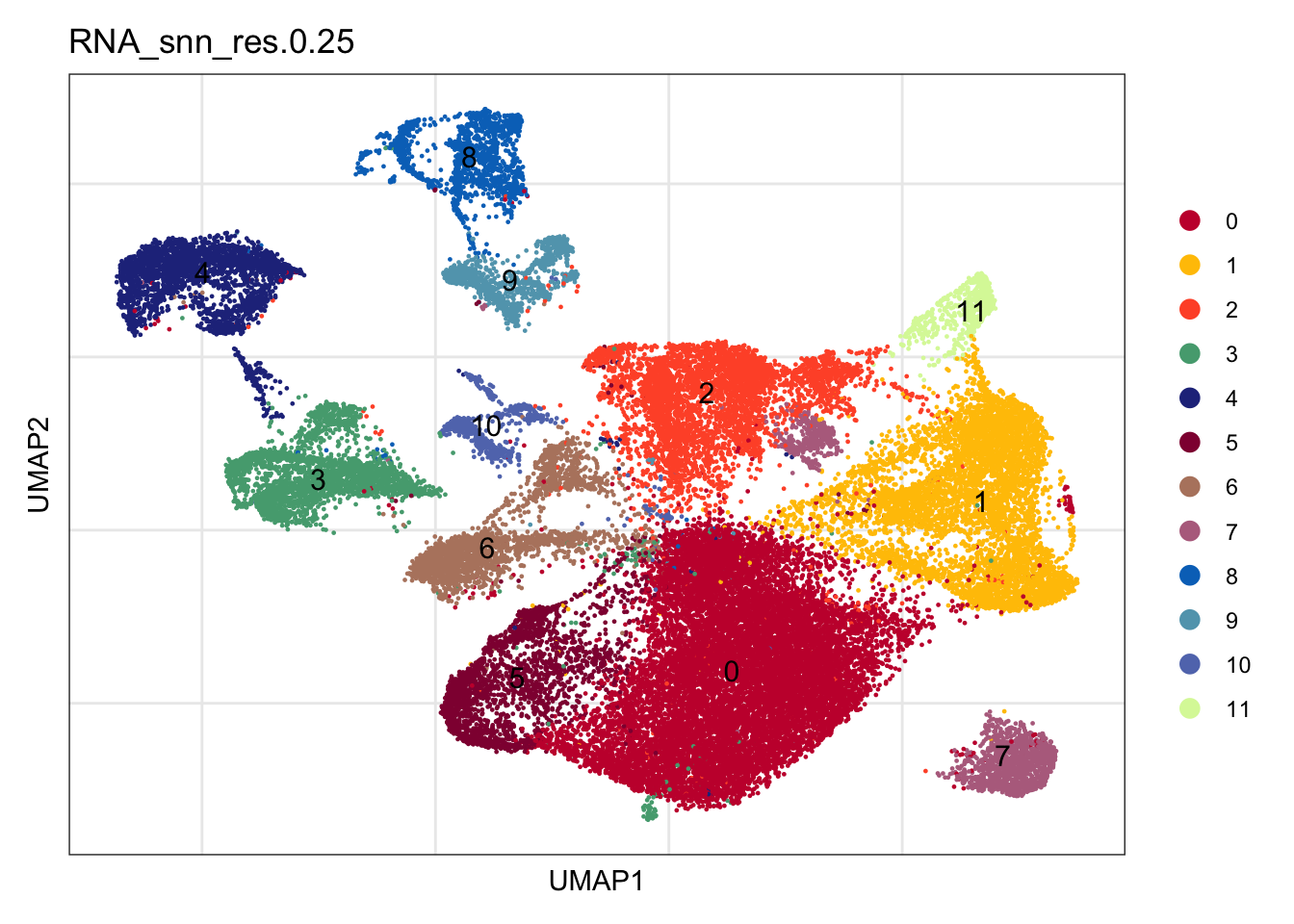
location
DimPlot(seuratE18fil, reduction = "umap", group.by = "location",
        cols = collocation)+
  theme_bw() +
  theme(axis.text = element_blank(), axis.ticks = element_blank(),
        panel.grid.minor = element_blank()) +
  xlab("UMAP1") +
  ylab("UMAP2")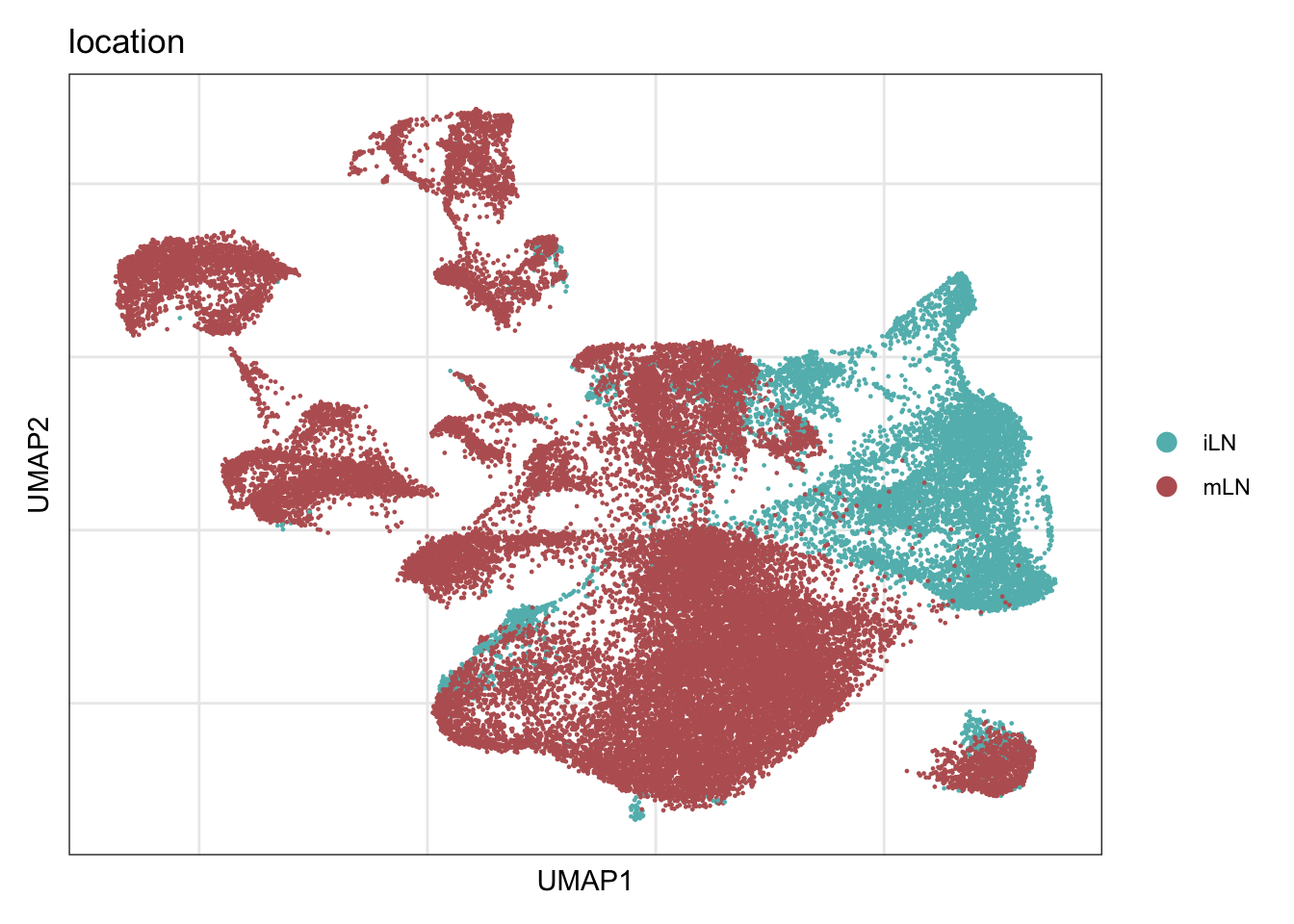
saveRDS(seuratE18fil, file=paste0(basedir,"/data/LNmLToRev_E18fil_seurat.rds"))subset EYFP expressing cells
seuratSub <- subset(seuratE18fil, Rosa26eyfp.Rosa26eyfp>0)
eyfpPos <- colnames(seuratSub)

seuratE18fil$EYFP <- "neg"
seuratE18fil$EYFP[which(colnames(seuratE18fil)%in%eyfpPos)] <- "pos"
table(seuratE18fil$dataset, seuratE18fil$EYFP)

table(seuratE18fil$EYFP)
seuratE18EYFPv2 <- subset(seuratE18fil, EYFP == "pos")
table(seuratE18EYFPv2$EYFP)

DimPlot(seuratE18EYFPv2, reduction = "umap", group.by = "RNA_snn_res.0.25",
        cols = colPal, label = TRUE)

#rerun seurat
seuratE18EYFPv2 <- NormalizeData (object = seuratE18EYFPv2)
seuratE18EYFPv2<- FindVariableFeatures(object = seuratE18EYFPv2)
seuratE18EYFPv2 <- ScaleData(object = seuratE18EYFPv2, verbose = TRUE)
seuratE18EYFPv2 <- RunPCA(object=seuratE18EYFPv2, npcs = 30, verbose = FALSE)
seuratE18EYFPv2 <- RunTSNE(object=seuratE18EYFPv2, reduction="pca", dims = 1:20)
seuratE18EYFPv2 <- RunUMAP(object=seuratE18EYFPv2, reduction="pca", dims = 1:20)
seuratE18EYFPv2 <- FindNeighbors(object = seuratE18EYFPv2, reduction = "pca", dims= 1:20)

res <- c(0.25, 0.6, 0.8, 0.4)
for (i in 1:length(res)) {
  seuratE18EYFPv2 <- FindClusters(object = seuratE18EYFPv2, resolution = res[i], random.seed = 1234)
}
saveRDS(seuratE18EYFPv2, file=paste0(basedir,"/data/E18_EYFPv2_seurat.rds")load object E18 EYFP+
fileNam <- paste0(basedir, "/data/E18_EYFPv2_seurat.rds")
seuratE18EYFPv2 <- readRDS(fileNam)
dimplot E18 EYFP+
clustering
Idents(seuratE18EYFPv2) <- seuratE18EYFPv2$RNA_snn_res.0.25
colPal <- c("#DAF7A6", "#FFC300", "#FF5733", "#C70039", "#900C3F", "#b66e8d",
            "#61a4ba", "#6178ba", "#54a87f",  "#25328a",
            "#b6856e", "#0073C2FF", "#EFC000FF", "#868686FF", "#CD534CFF",
            "#7AA6DCFF", "#003C67FF", "#8F7700FF", "#3B3B3BFF", "#A73030FF",
            "#4A6990FF")[1:length(unique(seuratE18EYFPv2$RNA_snn_res.0.25))]
names(colPal) <- unique(seuratE18EYFPv2$RNA_snn_res.0.25)

DimPlot(seuratE18EYFPv2, reduction = "umap", group.by = "RNA_snn_res.0.25",
        cols = colPal, label = TRUE)+
  theme_bw() +
  theme(axis.text = element_blank(), axis.ticks = element_blank(),
        panel.grid.minor = element_blank()) +
  xlab("UMAP1") +
  ylab("UMAP2")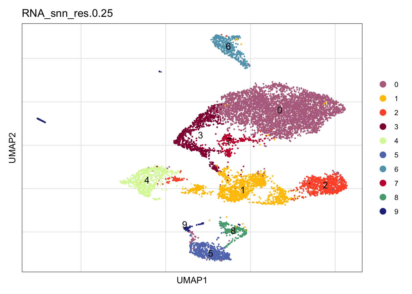
location
DimPlot(seuratE18EYFPv2, reduction = "umap", group.by = "location",
        cols = collocation)+
  theme_bw() +
  theme(axis.text = element_blank(), axis.ticks = element_blank(),
        panel.grid.minor = element_blank()) +
  xlab("UMAP1") +
  ylab("UMAP2")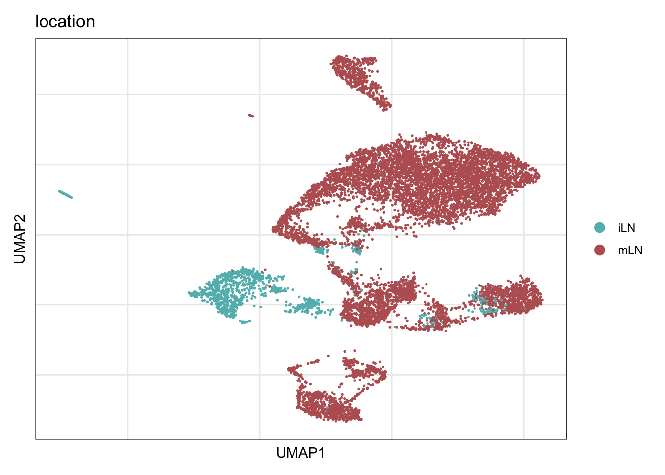
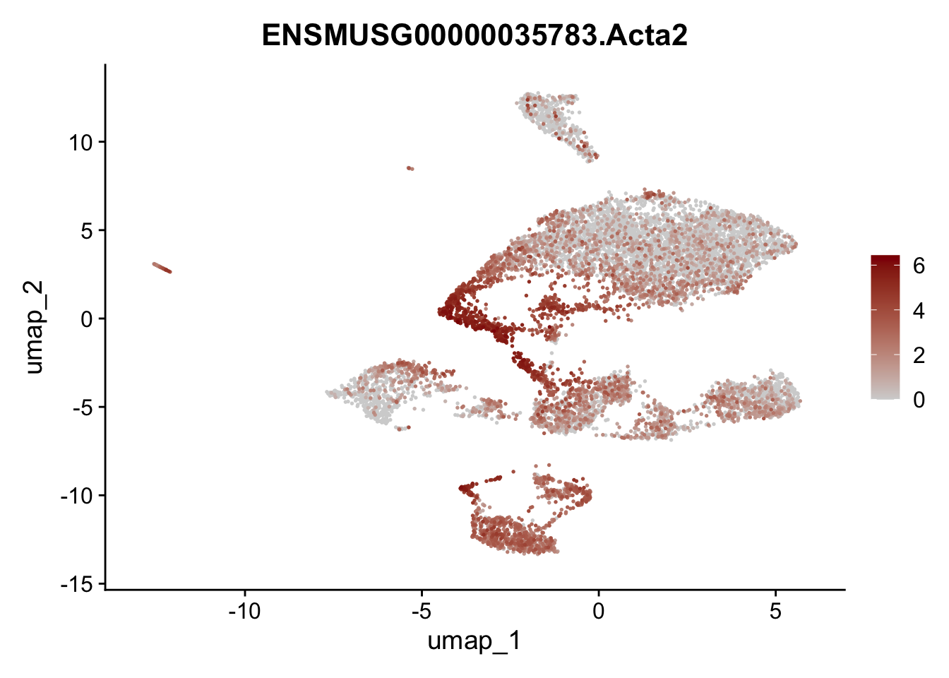
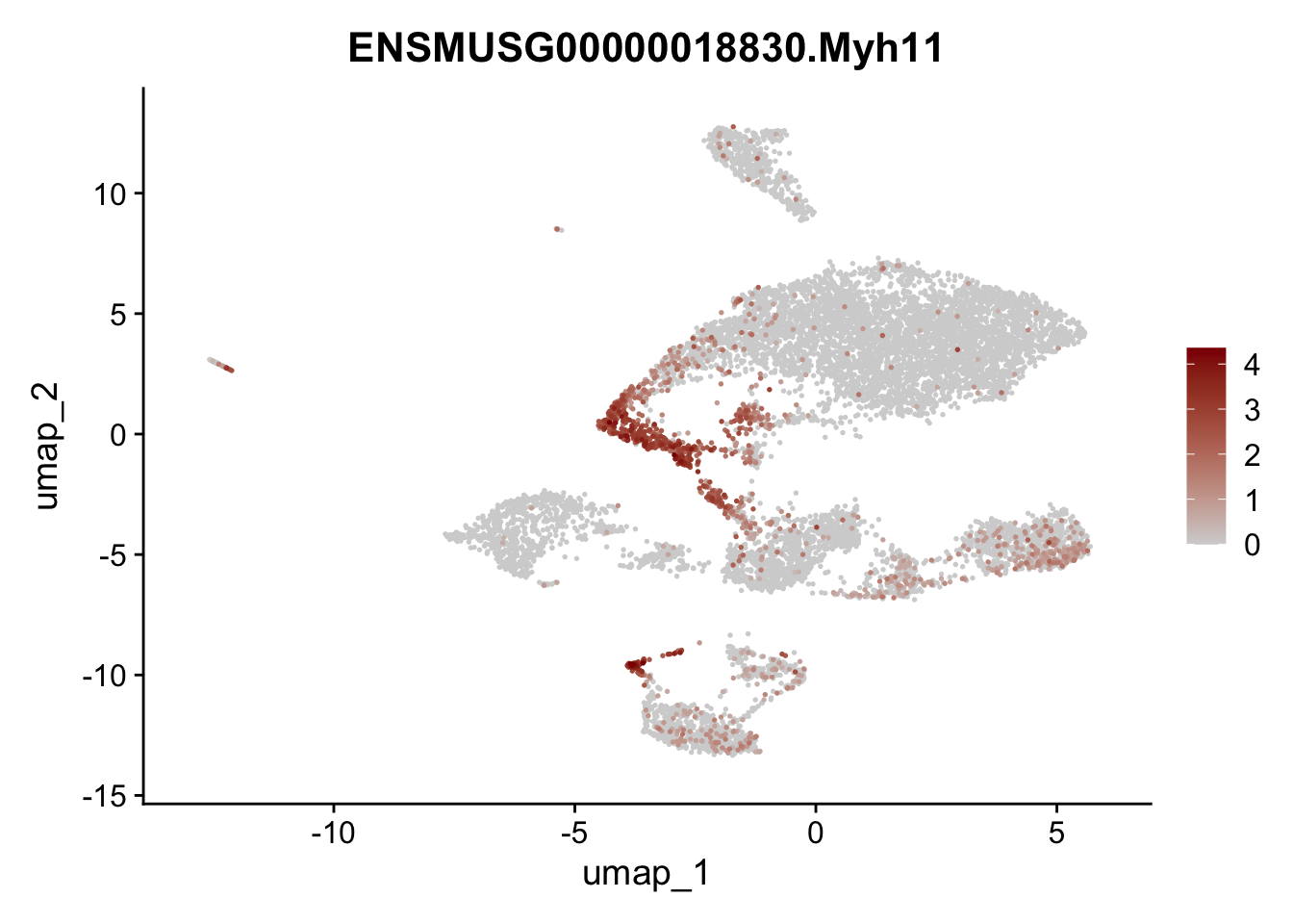
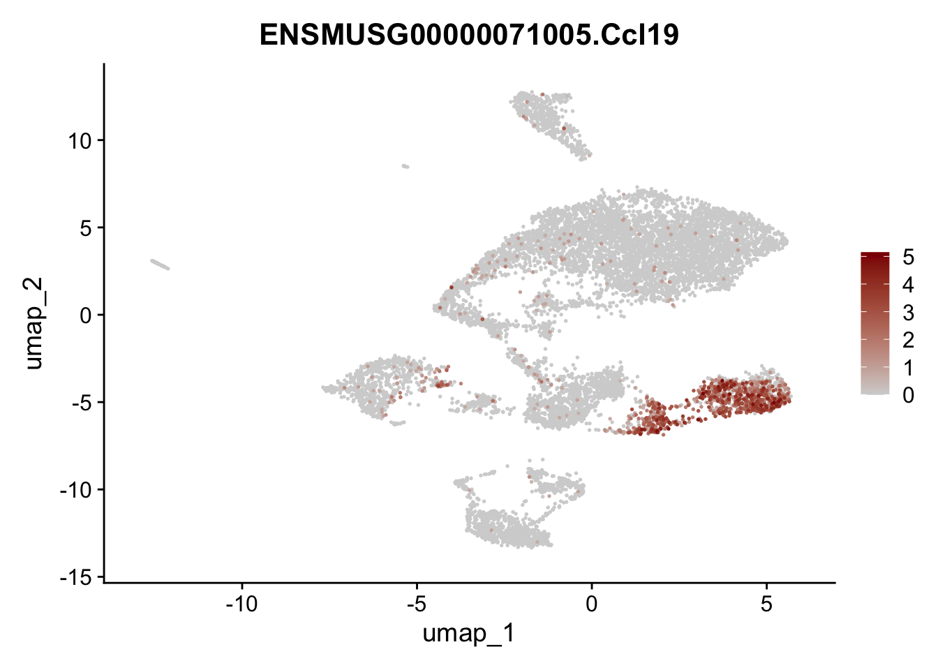
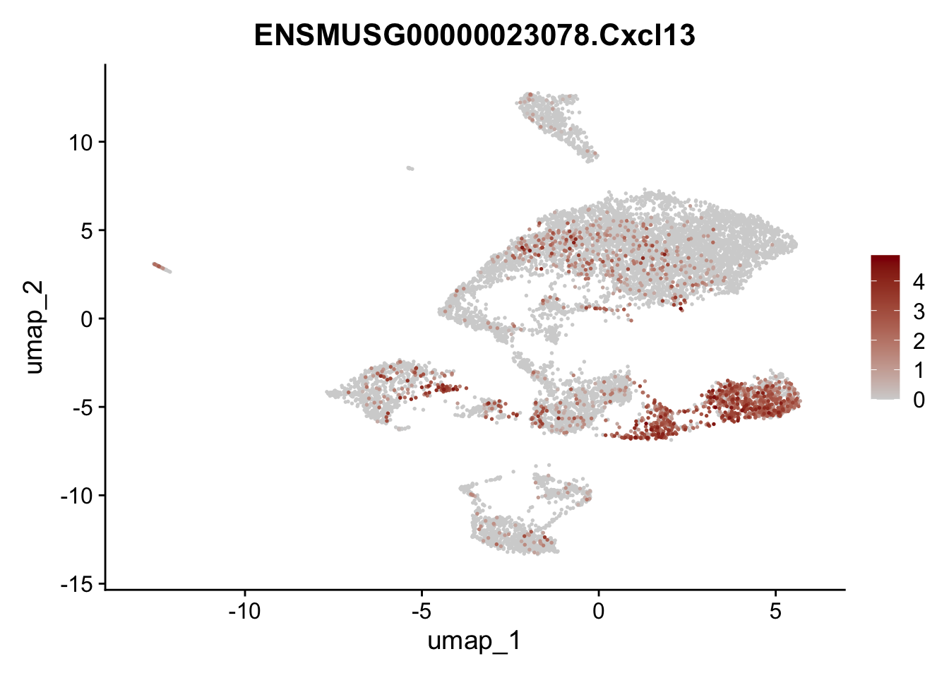
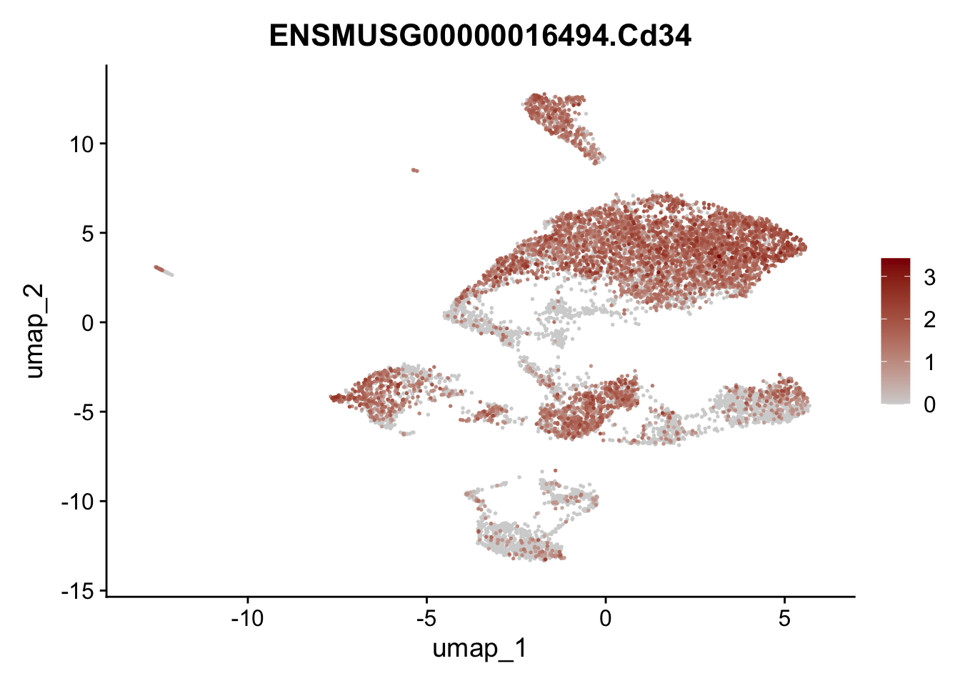
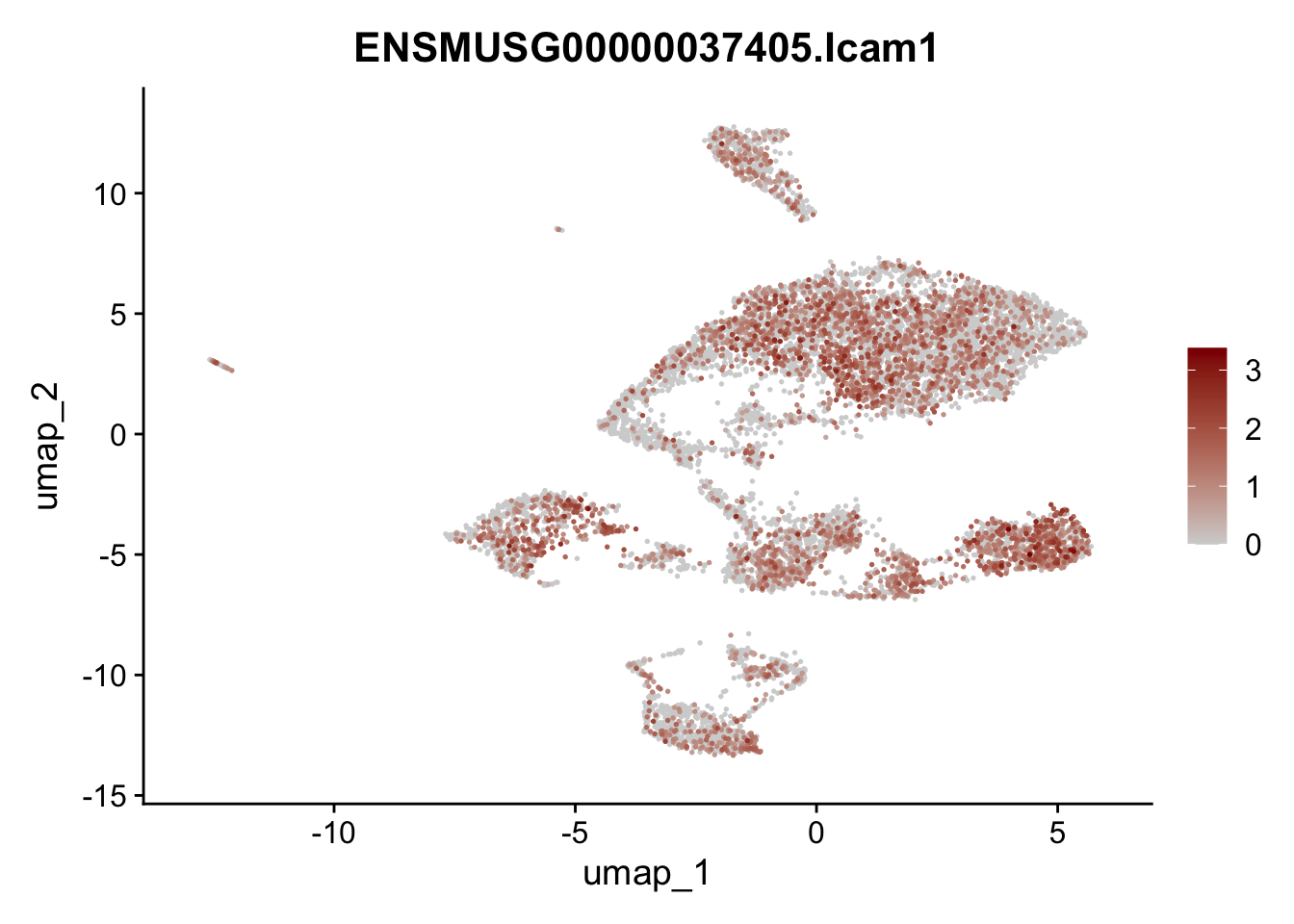
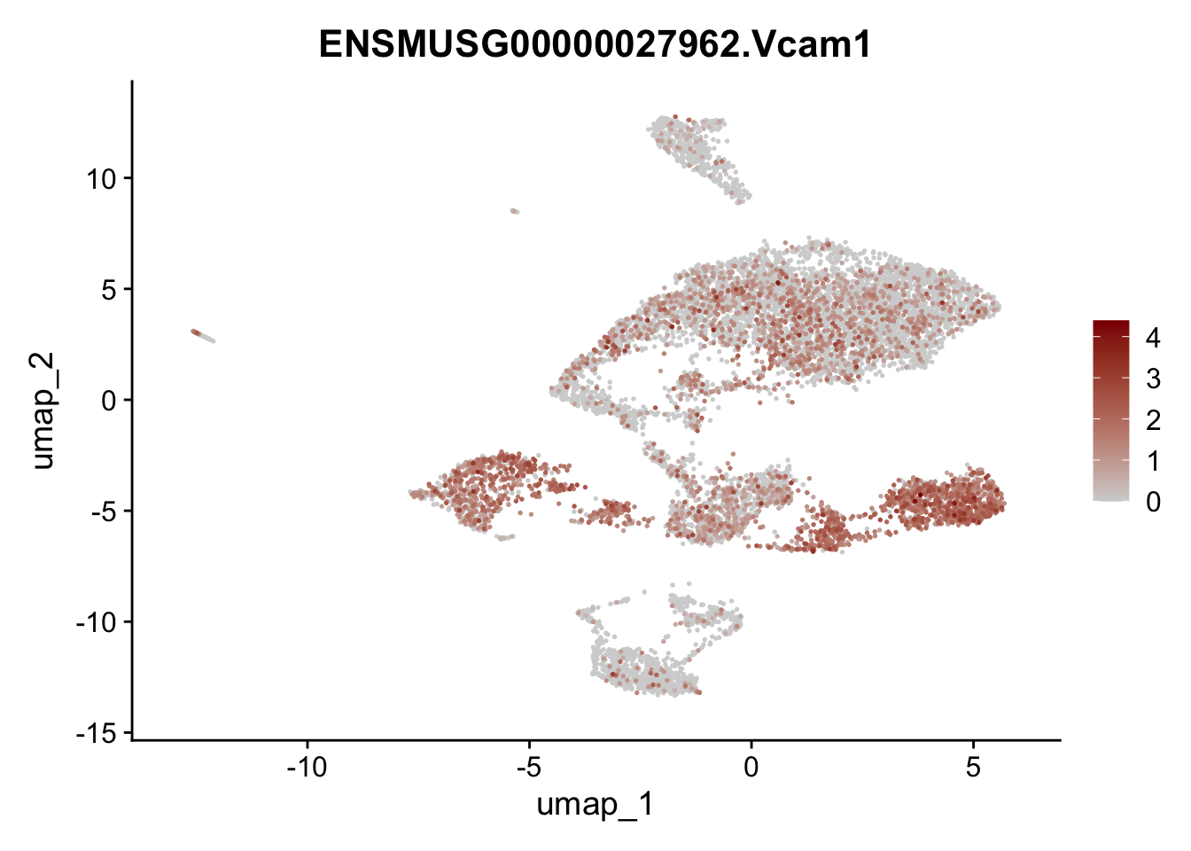
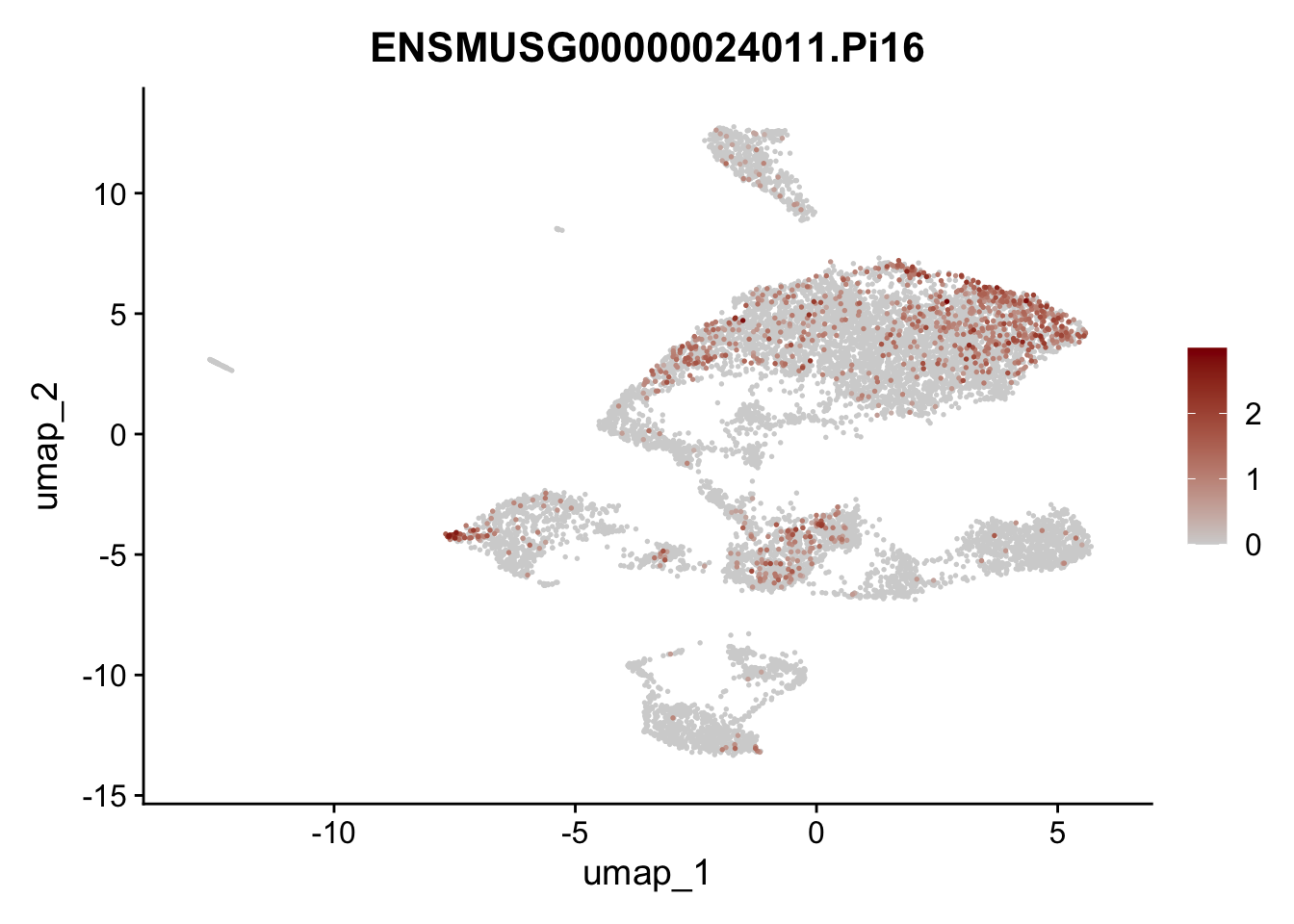
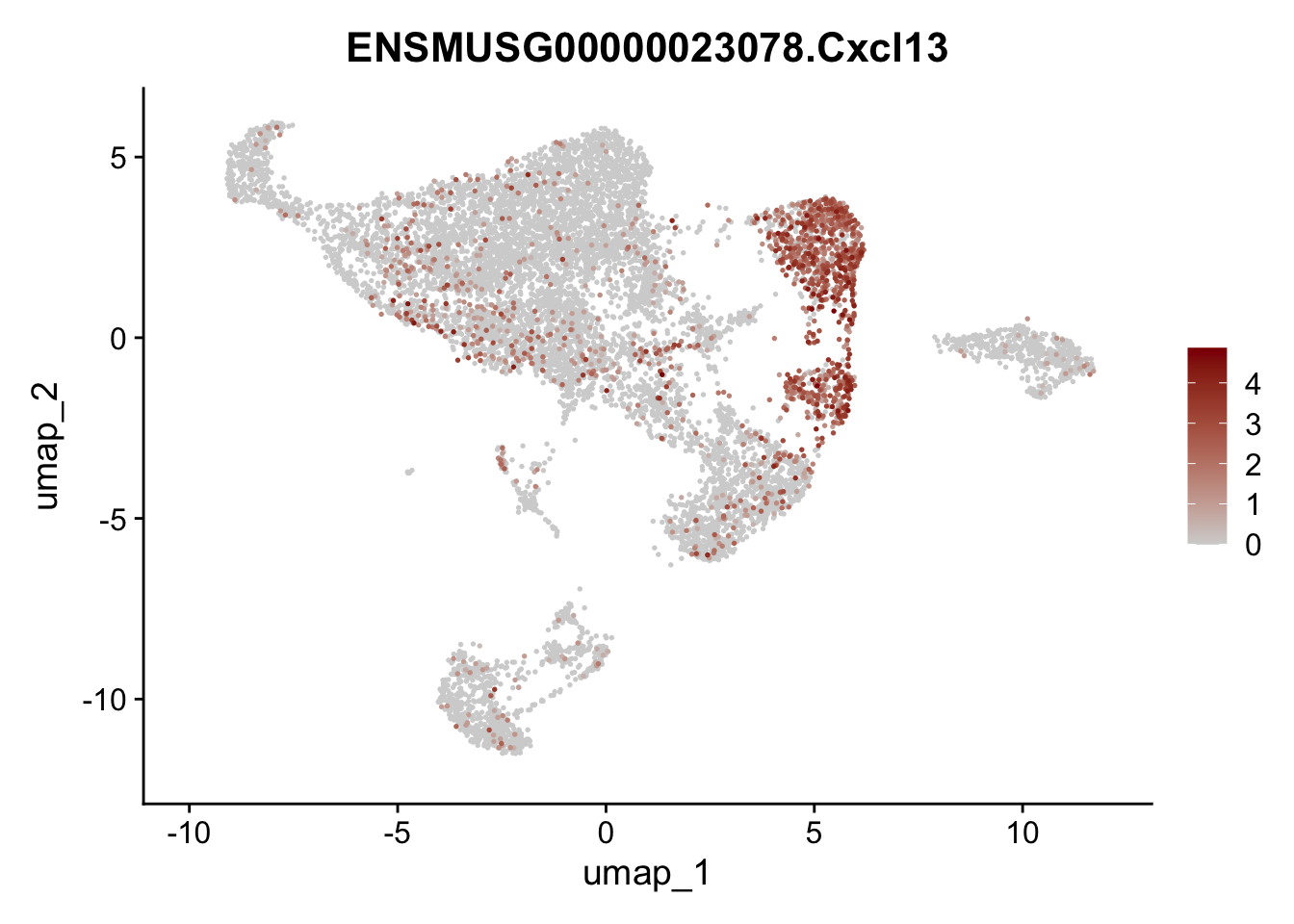
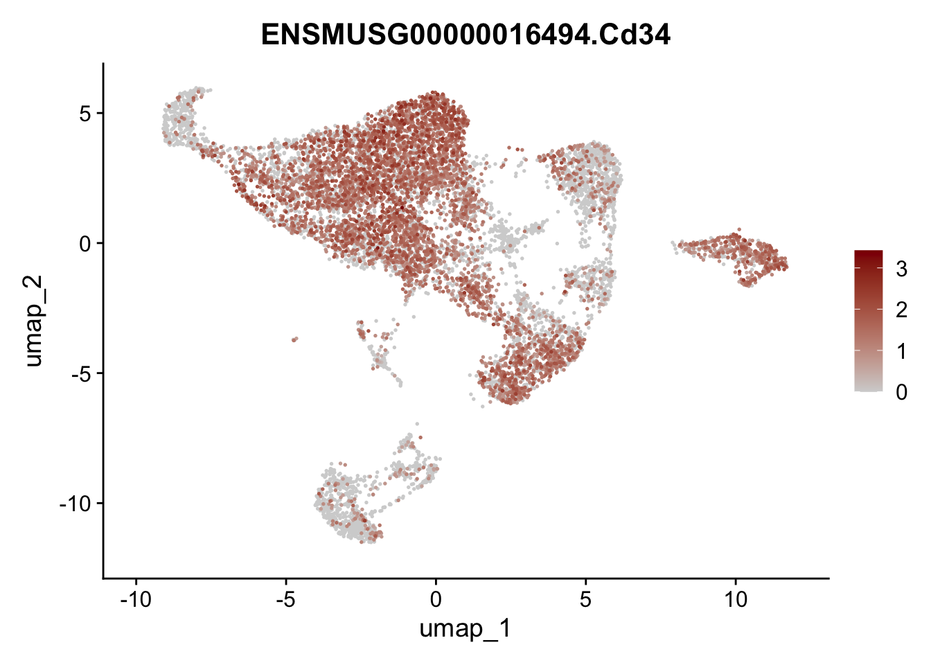
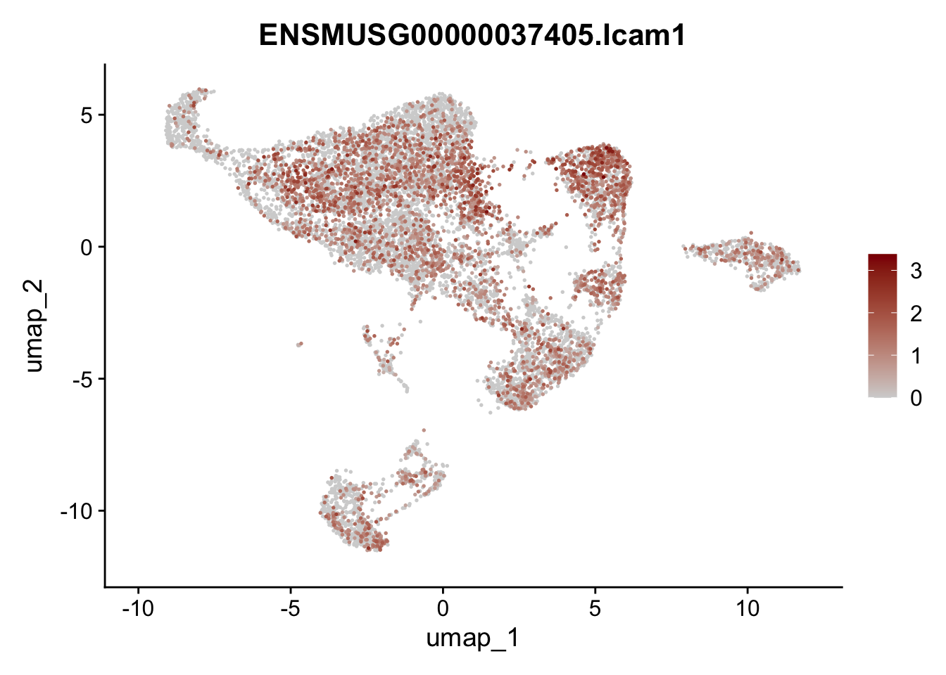
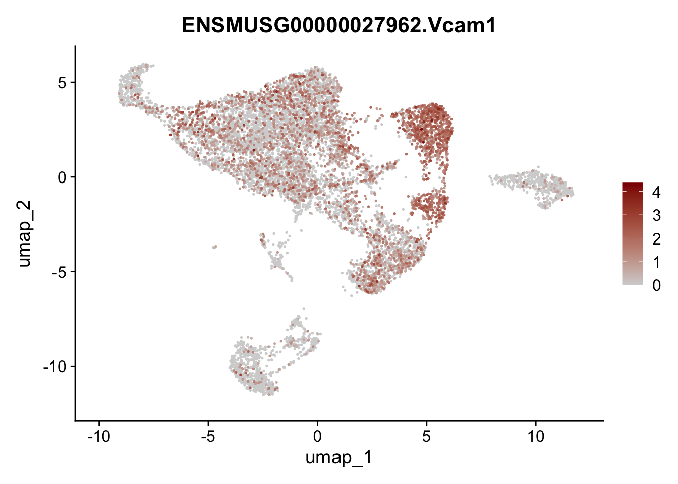
features E18 EYFP+
genes <- data.frame(gene=rownames(seuratE18EYFPv2)) %>%
    mutate(geneID=gsub("^.*\\.", "", gene))

selGenes <- data.frame(geneID=c("Rosa26eyfp", "Mki67", "Acta2", "Myh11", "Ccl19", "Cxcl13", "Cd34", "Icam1","Vcam1", "Pi16")) %>%
  left_join(., genes, by = "geneID")

pList <- sapply(selGenes$gene, function(x){
  p <- FeaturePlot(seuratE18EYFPv2, reduction = "umap",
            features = x,
            cols=c("lightgrey","darkred"),
            order = T)+
  theme(legend.position="right")
  plot(p)
})
integrate data across location
Idents(seuratE18EYFPv2) <- seuratE18EYFPv2$location

seurat.list <- SplitObject(object = seuratE18EYFPv2, split.by = "location")
for (i in 1:length(x = seurat.list)) {
    seurat.list[[i]] <- NormalizeData(object = seurat.list[[i]],
                                      verbose = FALSE)
    seurat.list[[i]] <- FindVariableFeatures(object = seurat.list[[i]],
        selection.method = "vst", nfeatures = 2000, verbose = FALSE)
}

seurat.anchors <- FindIntegrationAnchors(object.list = seurat.list, dims = 1:20)
seuratE18EYFPv2.int <- IntegrateData(anchorset = seurat.anchors, dims = 1:20)
DefaultAssay(object = seuratE18EYFPv2.int) <- "integrated"

## rerun seurat
seuratE18EYFPv2.int <- ScaleData(object = seuratE18EYFPv2.int, verbose = FALSE,
                         features = rownames(seuratE18EYFPv2.int))
seuratE18EYFPv2.int <- RunPCA(object = seuratE18EYFPv2.int, npcs = 20, verbose = FALSE)
seuratE18EYFPv2.int <- RunTSNE(object = seuratE18EYFPv2.int, recuction = "pca", dims = 1:20)
seuratE18EYFPv2.int <- RunUMAP(object = seuratE18EYFPv2.int, recuction = "pca", dims = 1:20)

seuratE18EYFPv2.int <- FindNeighbors(object = seuratE18EYFPv2.int, reduction = "pca", dims = 1:20)
res <- c(0.6, 0.8, 0.4, 0.25)
for (i in 1:length(res)){
  seuratE18EYFPv2.int <- FindClusters(object = seuratE18EYFPv2.int, resolution = res[i],
                              random.seed = 1234)
}
load object E18 EYFP+ integrated
fileNam <- paste0(basedir, "/data/E18EYFPv2_integrated_seurat.rds")
seuratE18EYFPv2.int <- readRDS(fileNam)
DefaultAssay(object = seuratE18EYFPv2.int) <- "RNA"
seuratE18EYFPv2.int$intCluster <- seuratE18EYFPv2.int$integrated_snn_res.0.25
Idents(seuratE18EYFPv2.int) <- seuratE18EYFPv2.int$intCluster
colPal <- c("#DAF7A6", "#FFC300", "#FF5733", "#C70039", "#900C3F", "#b66e8d",
"#61a4ba", "#6178ba", "#54a87f", "#25328a", "#b6856e",
"#ba6161", "#20714a", "#0073C2FF", "#EFC000FF", "#868686FF",
"#CD534CFF","#7AA6DCFF", "#003C67FF", "#8F7700FF", "#3B3B3BFF",
"#A73030FF", "#4A6990FF")[1:length(unique(seuratE18EYFPv2.int$intCluster))]
names(colPal) <- unique(seuratE18EYFPv2.int$intCluster)dimplot E18 EYFP+ int
clustering
DimPlot(seuratE18EYFPv2.int, reduction = "umap",
        label = T, shuffle = T, cols = colPal) +
  theme_bw() +
  theme(axis.text = element_blank(), axis.ticks = element_blank(),
        panel.grid.minor = element_blank()) +
  xlab("umap1") +
  ylab("umap2")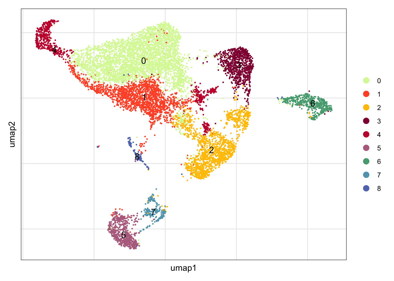
location
DimPlot(seuratE18EYFPv2.int, reduction = "umap", group.by = "location", cols = collocation,
        shuffle = T) +
  theme_bw() +
  theme(axis.text = element_blank(), axis.ticks = element_blank(),
        panel.grid.minor = element_blank()) +
  xlab("umap1") +
  ylab("umap2")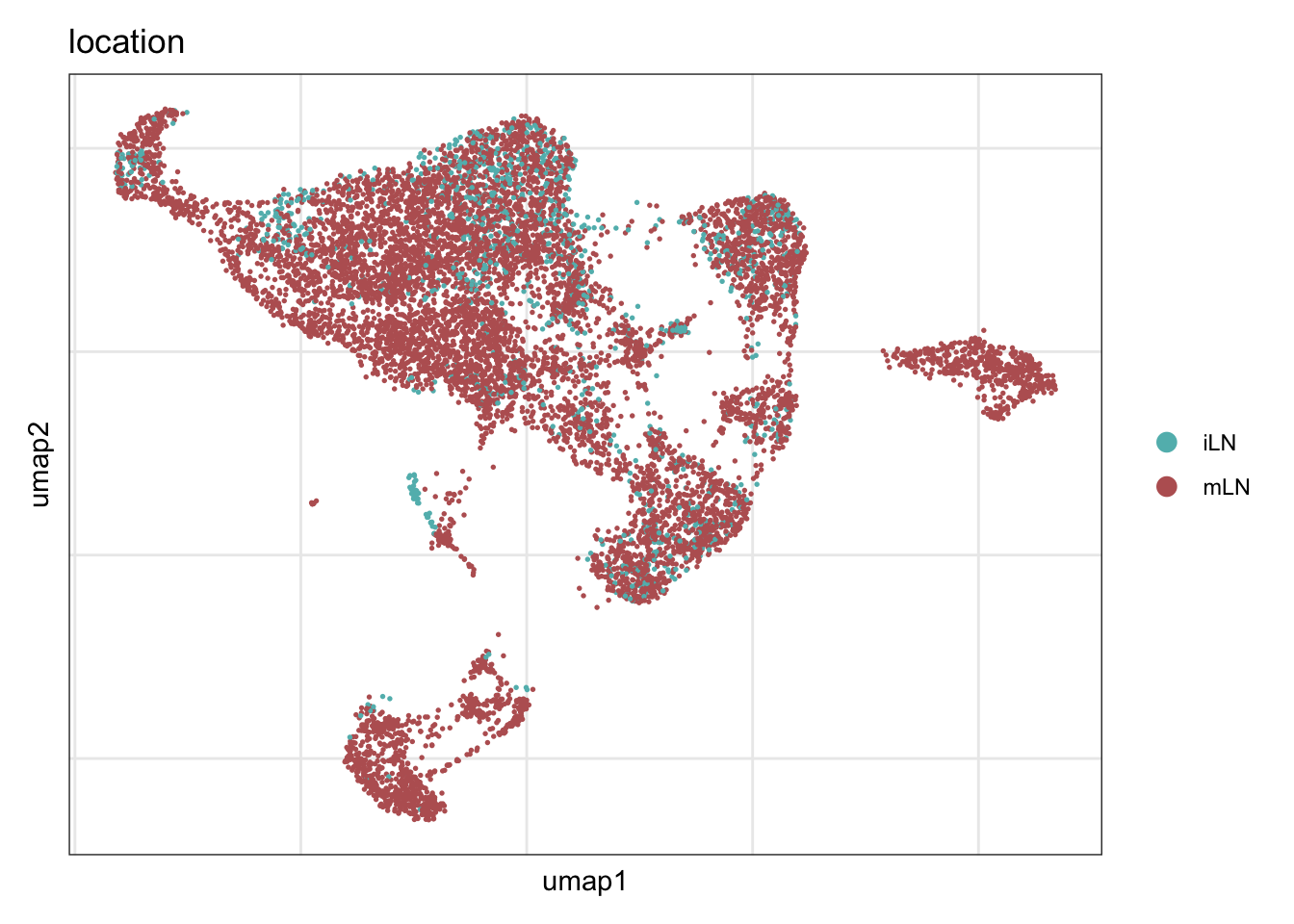
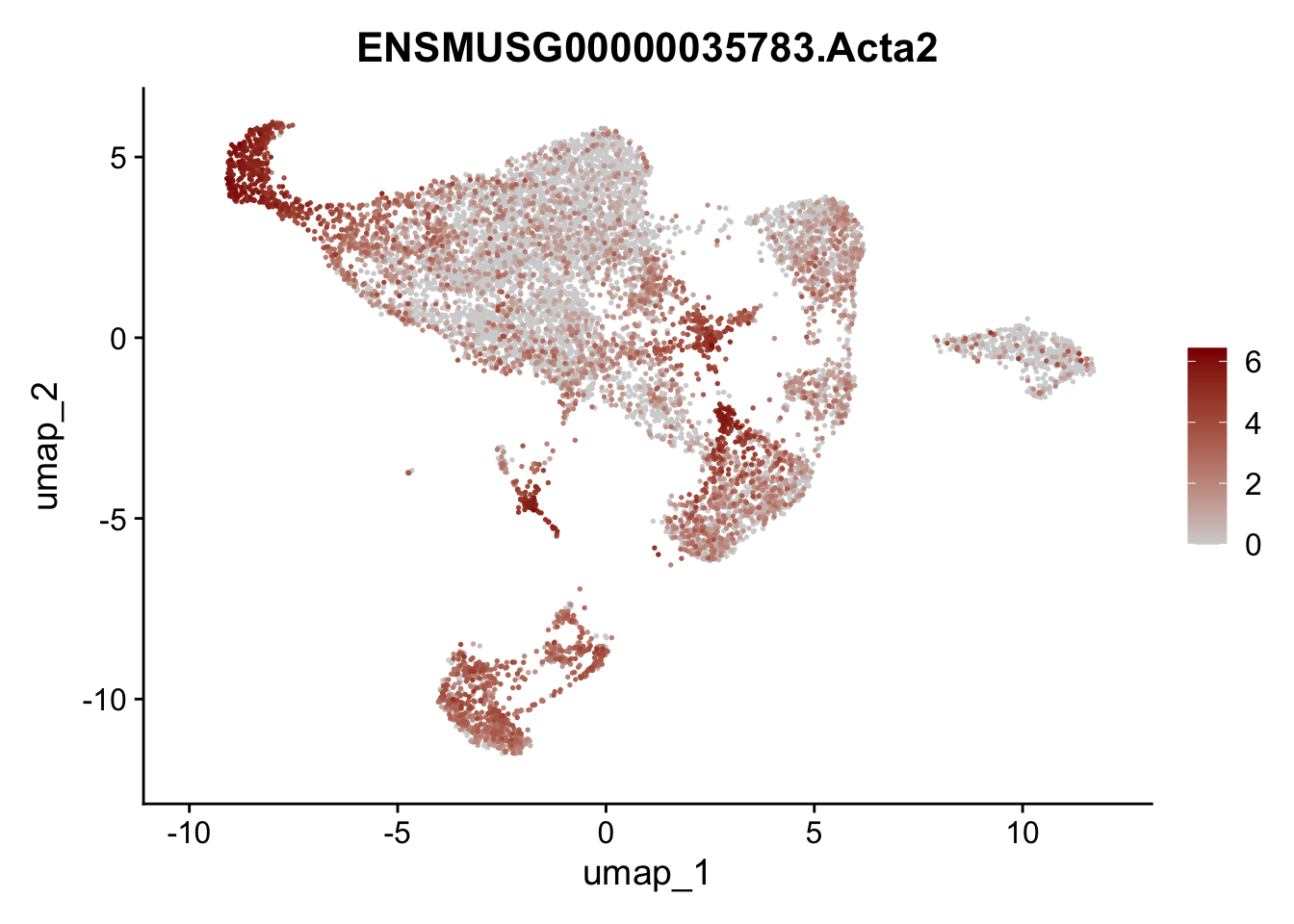
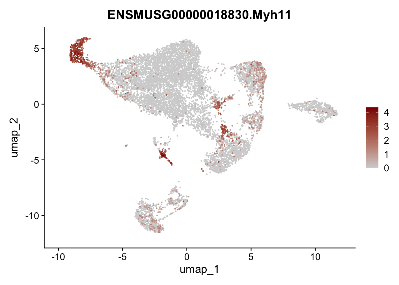
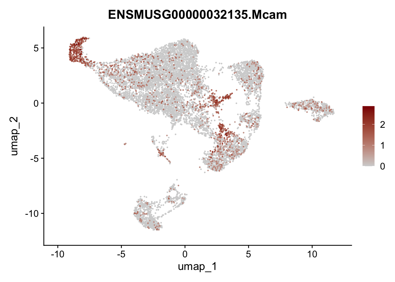
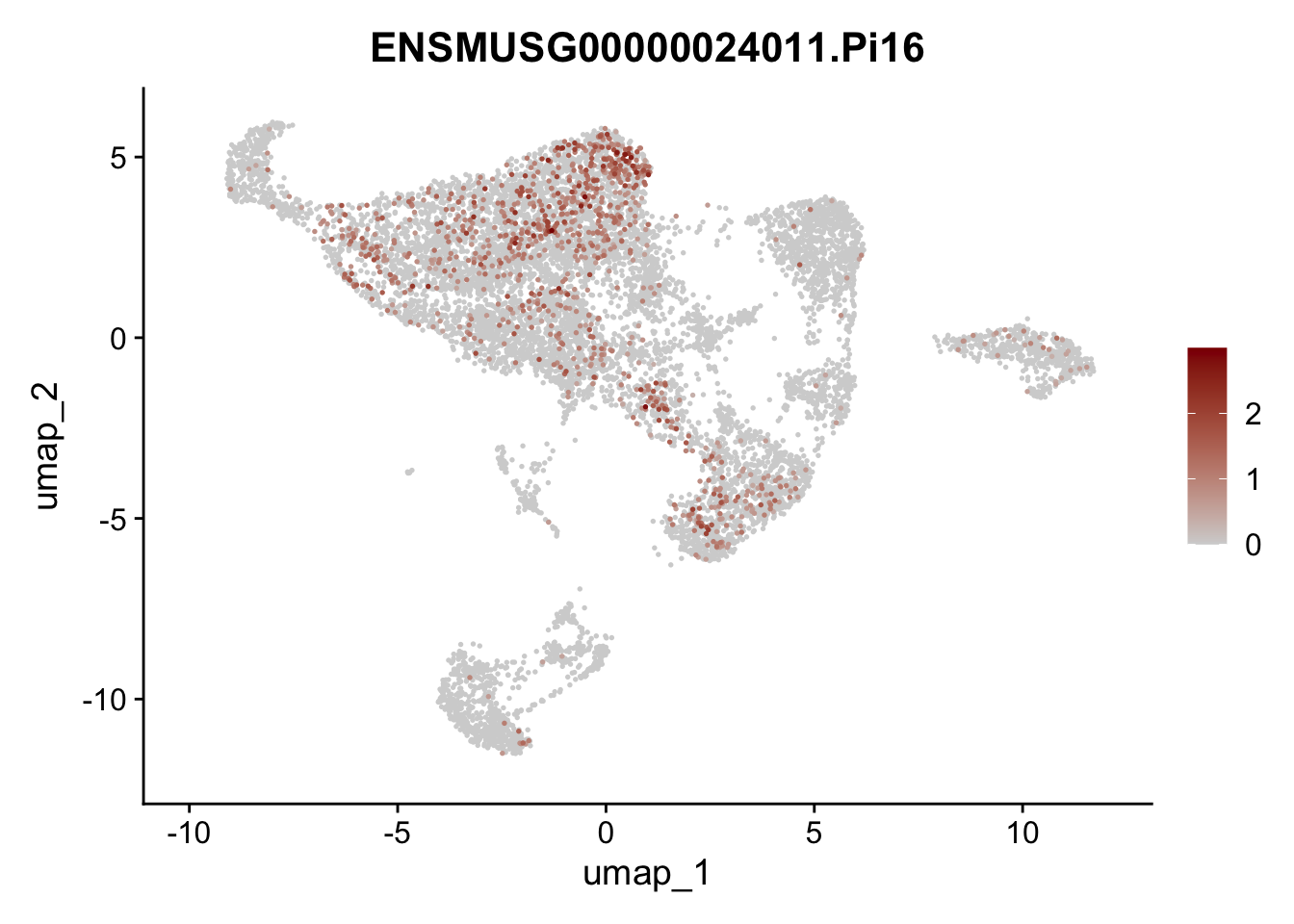
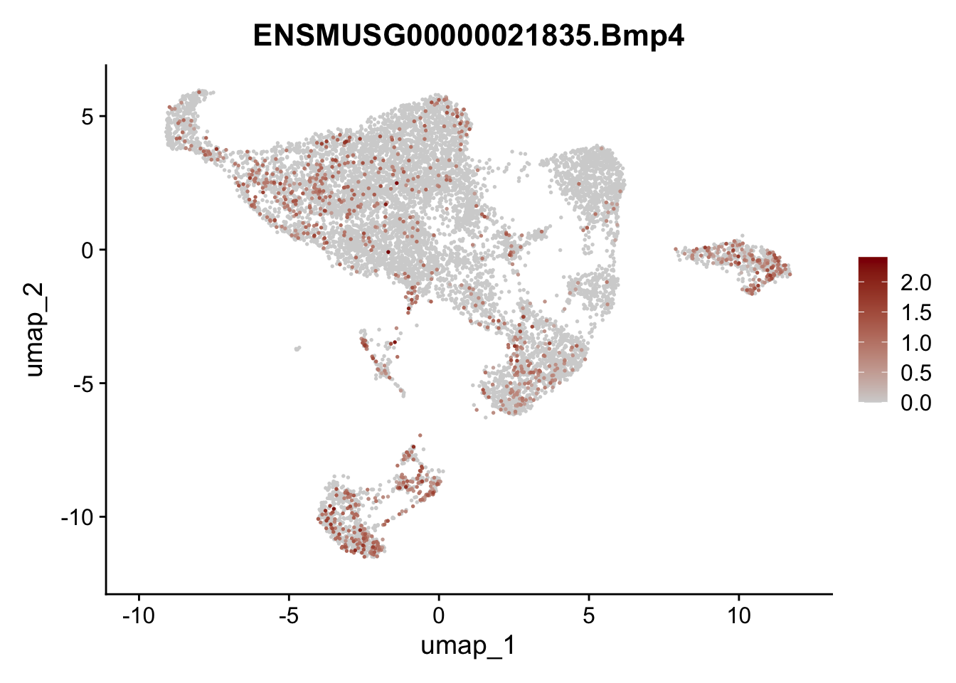
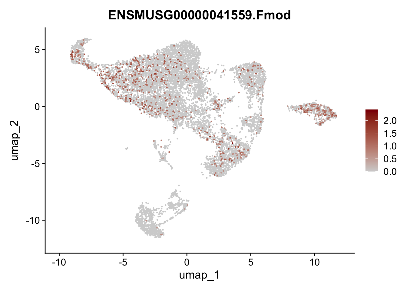
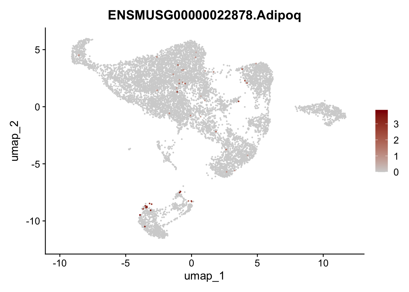
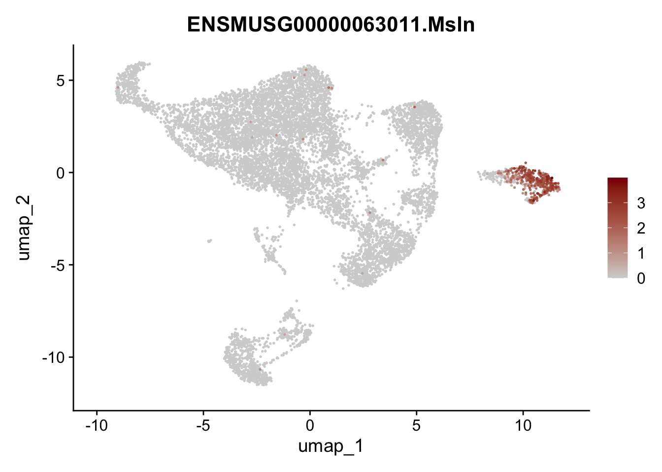
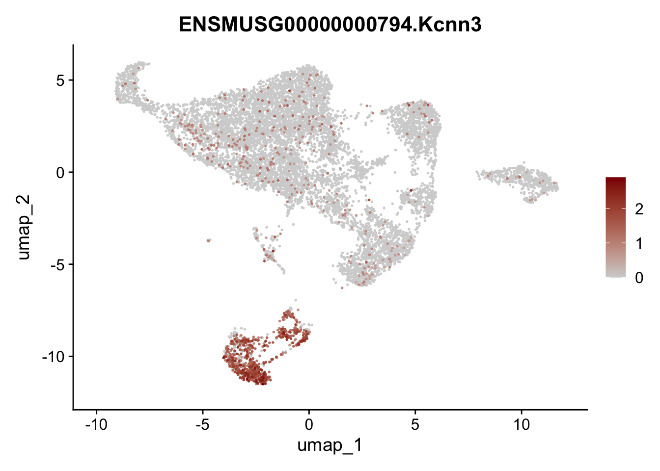
features E18 EYFP int
genes <- data.frame(gene=rownames(seuratE18EYFPv2.int)) %>%
    mutate(geneID=gsub("^.*\\.", "", gene))

selGenes <- data.frame(geneID=c("Rosa26eyfp", "Mki67", "Acta2", "Myh11", "Mcam", "Ccl19", "Cxcl13", "Cd34", "Icam1","Vcam1", "Pi16", "Bmp4", "Fmod", "Adipoq", "Msln", "Kcnn3")) %>%
  left_join(., genes, by = "geneID")

pList <- sapply(selGenes$gene, function(x){
  p <- FeaturePlot(seuratE18EYFPv2.int, reduction = "umap",
            features = x,
            cols=c("lightgrey","darkred"),
            order = T)+
  theme(legend.position="right")
  plot(p)
})
assign label
seuratE18EYFPv2.int$label <- "label"
seuratE18EYFPv2.int$label[which(seuratE18EYFPv2.int$intCluster == "0")] <- "cluster2"
seuratE18EYFPv2.int$label[which(seuratE18EYFPv2.int$intCluster == "1")] <- "cluster3"
seuratE18EYFPv2.int$label[which(seuratE18EYFPv2.int$intCluster == "2")] <- "Prolif"
seuratE18EYFPv2.int$label[which(seuratE18EYFPv2.int$intCluster == "3")] <- "cluster1"
seuratE18EYFPv2.int$label[which(seuratE18EYFPv2.int$intCluster == "4")] <- "cluster4"
seuratE18EYFPv2.int$label[which(seuratE18EYFPv2.int$intCluster == "5")] <- "Neuronal1"
seuratE18EYFPv2.int$label[which(seuratE18EYFPv2.int$intCluster == "6")] <- "Mesothelial"
seuratE18EYFPv2.int$label[which(seuratE18EYFPv2.int$intCluster == "7")] <- "Neuronal2"
seuratE18EYFPv2.int$label[which(seuratE18EYFPv2.int$intCluster == "8")] <- "cluster5"
table(seuratE18EYFPv2.int$label)
   cluster1    cluster2    cluster3    cluster4    cluster5 Mesothelial   Neuronal1   Neuronal2
        846        3781        1768         709         126         504         613         235
     Prolif
       1557
##order
seuratE18EYFPv2.int$label <- factor(seuratE18EYFPv2.int$label, levels = c("cluster1", "cluster2", "cluster3", "cluster4", "cluster5", "Neuronal1","Neuronal2", "Mesothelial", "Prolif"))
table(seuratE18EYFPv2.int$label)
   cluster1    cluster2    cluster3    cluster4    cluster5   Neuronal1   Neuronal2 Mesothelial
        846        3781        1768         709         126         613         235         504
     Prolif
       1557
colLab <- c("#900C3F","#b66e8d", "#003C67FF",
"#e3953d", "#714542", "#b6856e", "lightblue","grey", "black")
names(colLab) <- c("cluster1", "cluster2", "cluster3", "cluster4", "cluster5", "Neuronal1","Neuronal2", "Mesothelial", "Prolif")label
DimPlot(seuratE18EYFPv2.int, reduction = "umap", group.by = "label", cols = colLab)+
  theme_bw() +
  theme(axis.text = element_blank(), axis.ticks = element_blank(),
        panel.grid.minor = element_blank()) +
  xlab("UMAP1") +
  ylab("UMAP2")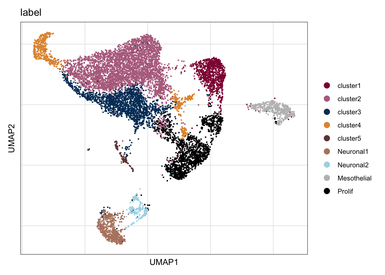
DimPlot(seuratE18EYFPv2.int, reduction = "umap", group.by = "label", pt.size=0.5,
        cols = colLab, shuffle = T)+
  theme_void()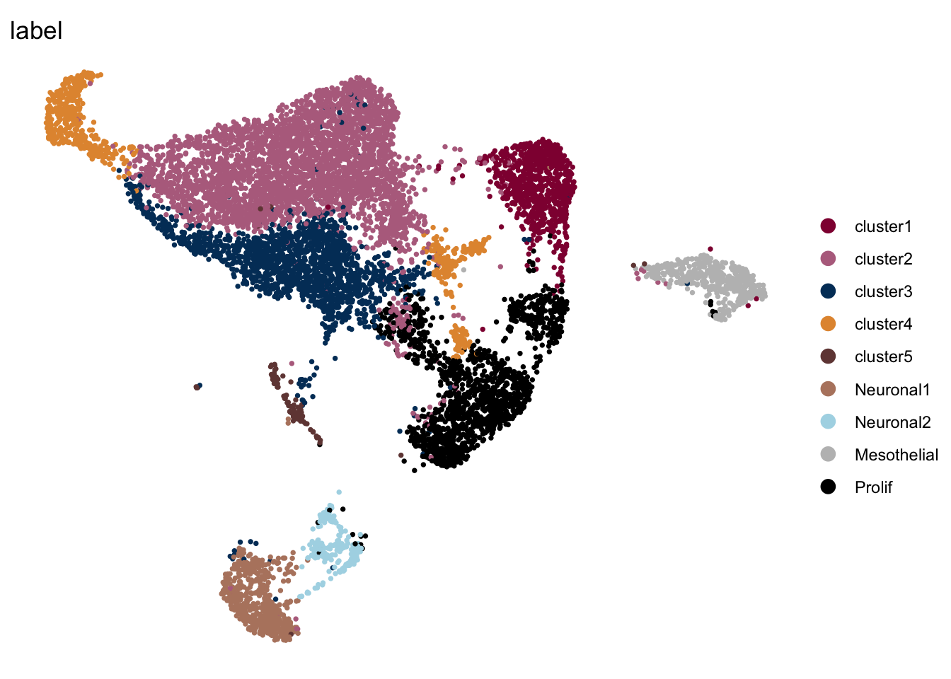
DimPlot(seuratE18EYFPv2.int, reduction = "umap", group.by = "label", pt.size=0.5,
        cols = colLab, shuffle = T)+
  theme_void() +
theme(legend.position = "none") 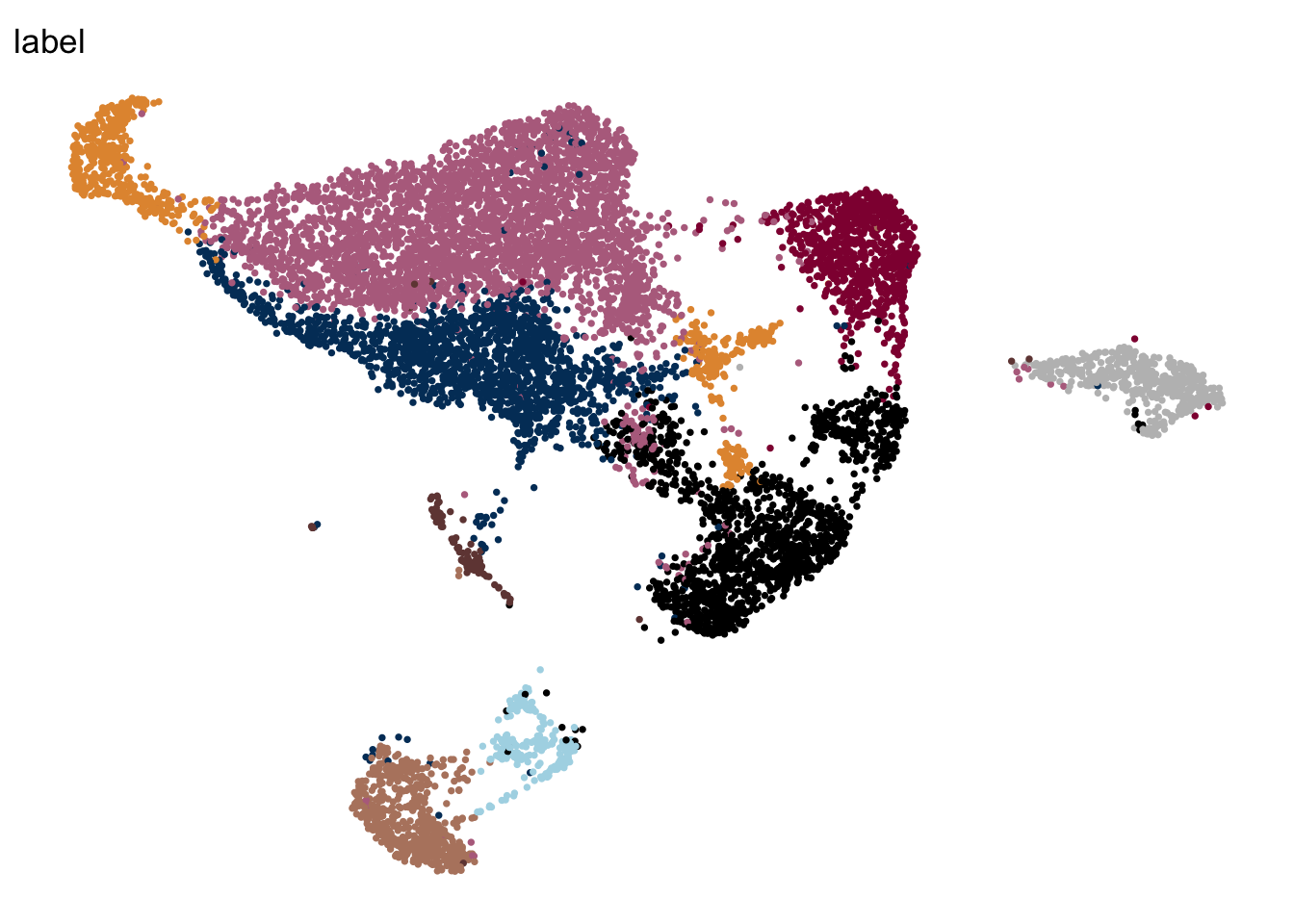
dotplot FRC marker E18 EYFP+ int
seurat_markers <- data.frame(gene=c("Fcgr2b","Fcer2a","Cr2","Cxcl13",
                                    "Slc7a11", "Ccl19",
                                    "Ccl21a", "Fmod", "Grem1", "Bmp4",
                                    "Tnfsf11", "Fbn2",
                                    "Pltp" ,"C1rb", "Lepr", "Ptn",
                                     "Nr4a1", "Cxcl10", "Cxcl9",
                                    "F3", "Fbln1", "Gdf10", "Adamtsl1",
                                    "Col15a1",  "Cd34",
                                    "Igfbp6", "Pi16", "Thy1", "Dpp4", "Sema3c",
                                    "Acta2", "Myh11", "Mcam", "Itga7", "Esam", "Rgs4", "Adipoq", "Mki67", "Msln", "Kcnn3", "Tcf21"
                                    ))

genes <- data.frame(geneID=rownames(seuratE18EYFPv2.int)) %>%
  mutate(gene=gsub(".*\\.", "",  geneID))

markerAll <- seurat_markers %>% left_join(., genes, by="gene")


## Dotplot all
Idents(seuratE18EYFPv2.int) <- seuratE18EYFPv2.int$label

DotPlot(seuratE18EYFPv2.int, assay="RNA", features = rev(markerAll$geneID), scale =T,
        cluster.idents = F) +
  scale_color_viridis_c() +
  coord_flip() +
  theme(axis.text.x = element_text(angle = 90, hjust = 1)) +
  scale_x_discrete(breaks=rev(markerAll$geneID), labels=rev(markerAll$gene)) +
  xlab("") + ylab("")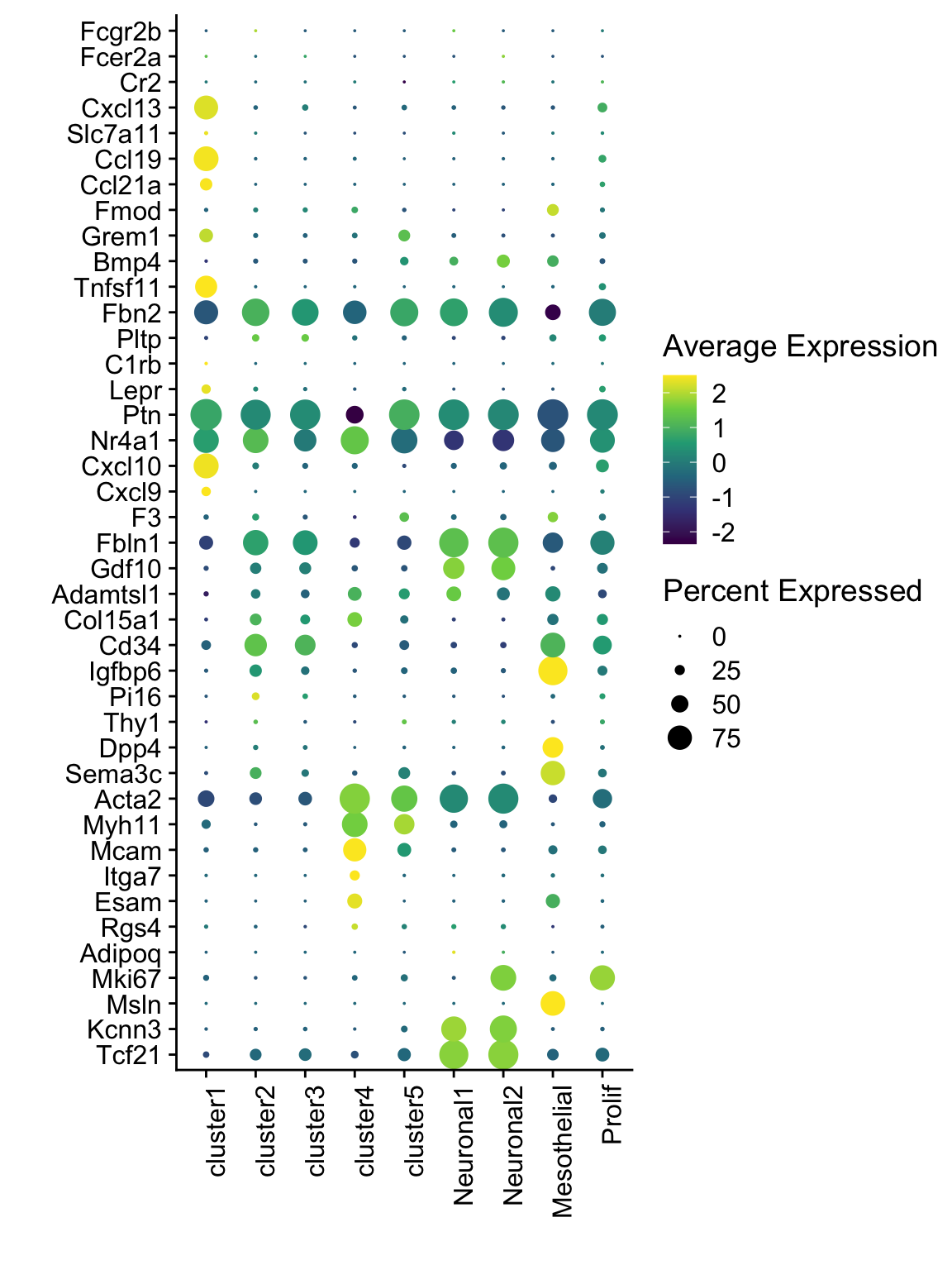
saveRDS(seuratE18EYFPv2.int, file=paste0(basedir,"/data/E18EYFPv2_integrated_seurat.rds")subset FRCs and rerun
table(seuratE18EYFPv2.int$label)
   cluster1    cluster2    cluster3    cluster4    cluster5   Neuronal1   Neuronal2 Mesothelial
        846        3781        1768         709         126         613         235         504
     Prolif
       1557
seuratE18EYFPv2.int <- subset(seuratE18EYFPv2.int, label %in% c("Neuronal1", "Neuronal2", "Mesothelial"), invert = TRUE)
table(seuratE18EYFPv2.int$label)
cluster1 cluster2 cluster3 cluster4 cluster5   Prolif
     846     3781     1768      709      126     1557
## rerun seurat
DefaultAssay(object = seuratE18EYFPv2.int) <- "integrated"
seuratE18EYFPv2.int <- ScaleData(object = seuratE18EYFPv2.int, verbose = FALSE,
features = rownames(seuratE18EYFPv2.int))
seuratE18EYFPv2.int <- RunPCA(object = seuratE18EYFPv2.int, npcs = 20, verbose = FALSE)
seuratE18EYFPv2.int <- RunTSNE(object = seuratE18EYFPv2.int, recuction = "pca", dims = 1:20)
seuratE18EYFPv2.int <- RunUMAP(object = seuratE18EYFPv2.int, recuction = "pca", dims = 1:20)
seuratE18EYFPv2.int <- FindNeighbors(object = seuratE18EYFPv2.int, reduction = "pca", dims = 1:20)
res <- c(0.1, 0.6, 0.8, 0.4, 0.25)
for (i in 1:length(res)){
seuratE18EYFPv2.int <- FindClusters(object = seuratE18EYFPv2.int, resolution = res[i],
random.seed = 1234)
}Modularity Optimizer version 1.3.0 by Ludo Waltman and Nees Jan van Eck
Number of nodes: 8787
Number of edges: 284718
Running Louvain algorithm...
Maximum modularity in 10 random starts: 0.9414
Number of communities: 5
Elapsed time: 1 seconds
Modularity Optimizer version 1.3.0 by Ludo Waltman and Nees Jan van Eck
Number of nodes: 8787
Number of edges: 284718
Running Louvain algorithm...
Maximum modularity in 10 random starts: 0.8396
Number of communities: 11
Elapsed time: 1 seconds
Modularity Optimizer version 1.3.0 by Ludo Waltman and Nees Jan van Eck
Number of nodes: 8787
Number of edges: 284718
Running Louvain algorithm...
Maximum modularity in 10 random starts: 0.8161
Number of communities: 13
Elapsed time: 1 seconds
Modularity Optimizer version 1.3.0 by Ludo Waltman and Nees Jan van Eck
Number of nodes: 8787
Number of edges: 284718
Running Louvain algorithm...
Maximum modularity in 10 random starts: 0.8664
Number of communities: 10
Elapsed time: 0 seconds
Modularity Optimizer version 1.3.0 by Ludo Waltman and Nees Jan van Eck
Number of nodes: 8787
Number of edges: 284718
Running Louvain algorithm...
Maximum modularity in 10 random starts: 0.8921
Number of communities: 8
Elapsed time: 1 secondsDefaultAssay(object = seuratE18EYFPv2.int) <- "RNA"
seuratE18EYFPv2.int$intCluster <- seuratE18EYFPv2.int$integrated_snn_res.0.1
Idents(seuratE18EYFPv2.int) <- seuratE18EYFPv2.int$intCluster
colPal <- c("#DAF7A6", "#FFC300", "#FF5733", "#C70039", "#900C3F", "#b66e8d",
"#61a4ba", "#6178ba", "#54a87f", "#25328a", "#b6856e",
"#ba6161", "#20714a", "#0073C2FF", "#EFC000FF", "#868686FF",
"#CD534CFF","#7AA6DCFF", "#003C67FF", "#8F7700FF", "#3B3B3BFF",
"#A73030FF", "#4A6990FF")[1:length(unique(seuratE18EYFPv2.int$intCluster))]
names(colPal) <- unique(seuratE18EYFPv2.int$intCluster)dimplot E18 EYFP+ fil
clustering
DimPlot(seuratE18EYFPv2.int, reduction = "umap",
        label = T, shuffle = T, cols = colPal) +
  theme_bw() +
  theme(axis.text = element_blank(), axis.ticks = element_blank(),
        panel.grid.minor = element_blank()) +
  xlab("umap1") +
  ylab("umap2")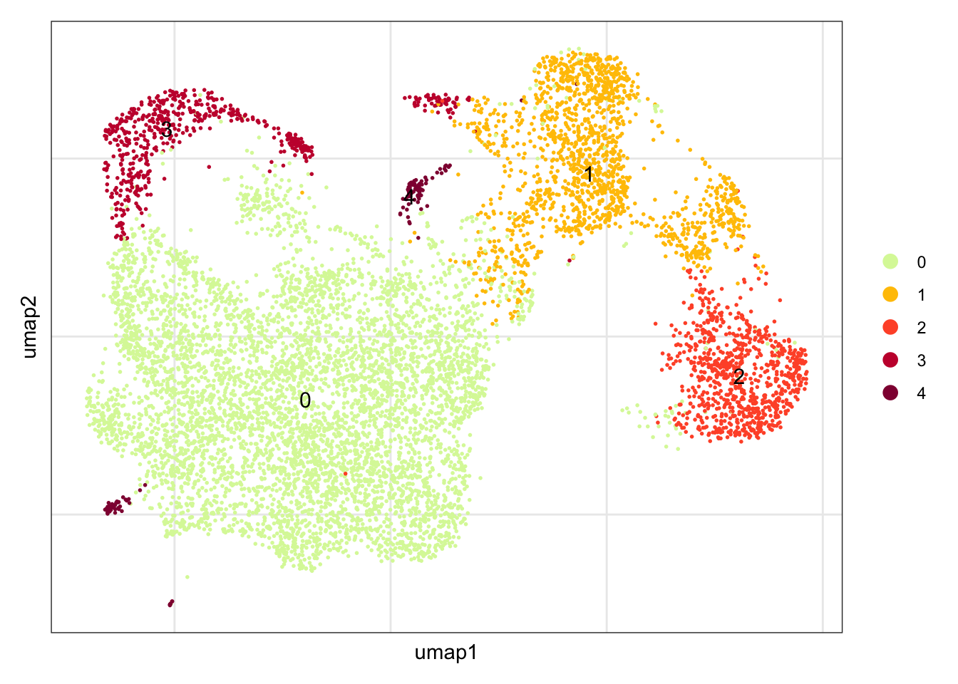
location
DimPlot(seuratE18EYFPv2.int, reduction = "umap", group.by = "location", cols = collocation,
        shuffle = T) +
  theme_bw() +
  theme(axis.text = element_blank(), axis.ticks = element_blank(),
        panel.grid.minor = element_blank()) +
  xlab("umap1") +
  ylab("umap2")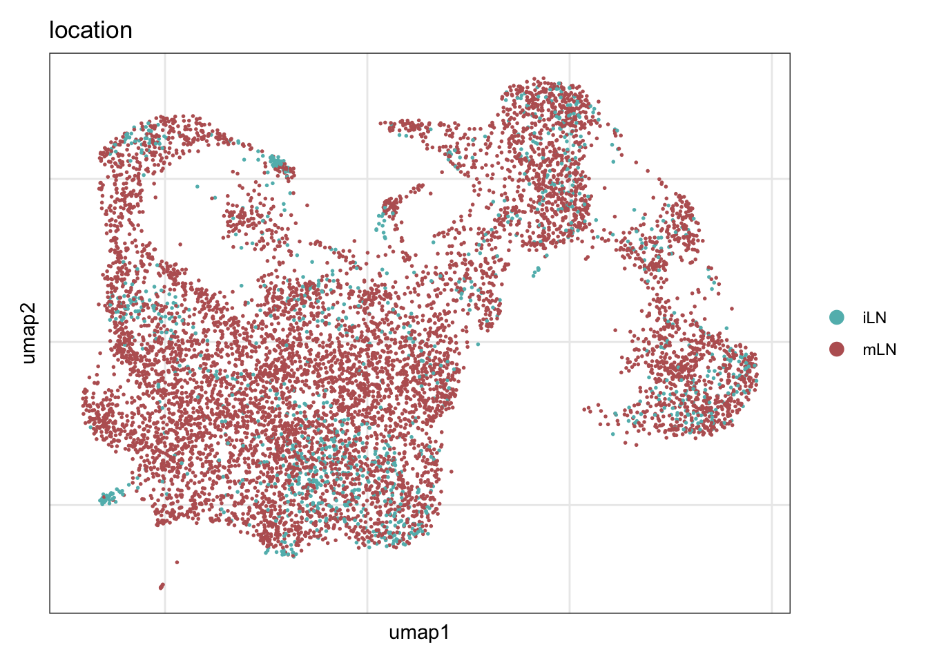
assign label
seuratE18EYFPv2.int$label <- "label"
seuratE18EYFPv2.int$label[which(seuratE18EYFPv2.int$intCluster == "0")] <- "cluster3"
seuratE18EYFPv2.int$label[which(seuratE18EYFPv2.int$intCluster == "1")] <- "cluster1"
seuratE18EYFPv2.int$label[which(seuratE18EYFPv2.int$intCluster == "2")] <- "cluster2"
seuratE18EYFPv2.int$label[which(seuratE18EYFPv2.int$intCluster == "3")] <- "cluster4"
seuratE18EYFPv2.int$label[which(seuratE18EYFPv2.int$intCluster == "4")] <- "cluster5"
table(seuratE18EYFPv2.int$label)
cluster1 cluster2 cluster3 cluster4 cluster5
    1523      843     5735      563      123
##order
seuratE18EYFPv2.int$label <- factor(seuratE18EYFPv2.int$label, levels = c("cluster2", "cluster3", "cluster4", "cluster5", "cluster1"))
table(seuratE18EYFPv2.int$label)
cluster2 cluster3 cluster4 cluster5 cluster1
     843     5735      563      123     1523
colLab <- c("#900C3F","#b66e8d", "#003C67FF",
"#e3953d", "#714542", "#b6856e")
names(colLab) <- c("cluster2", "cluster3", "cluster1", "cluster4", "cluster5")label
DimPlot(seuratE18EYFPv2.int, reduction = "umap", group.by = "label", cols = colLab)+
  theme_bw() +
  theme(axis.text = element_blank(), axis.ticks = element_blank(),
        panel.grid.minor = element_blank()) +
  xlab("UMAP1") +
  ylab("UMAP2")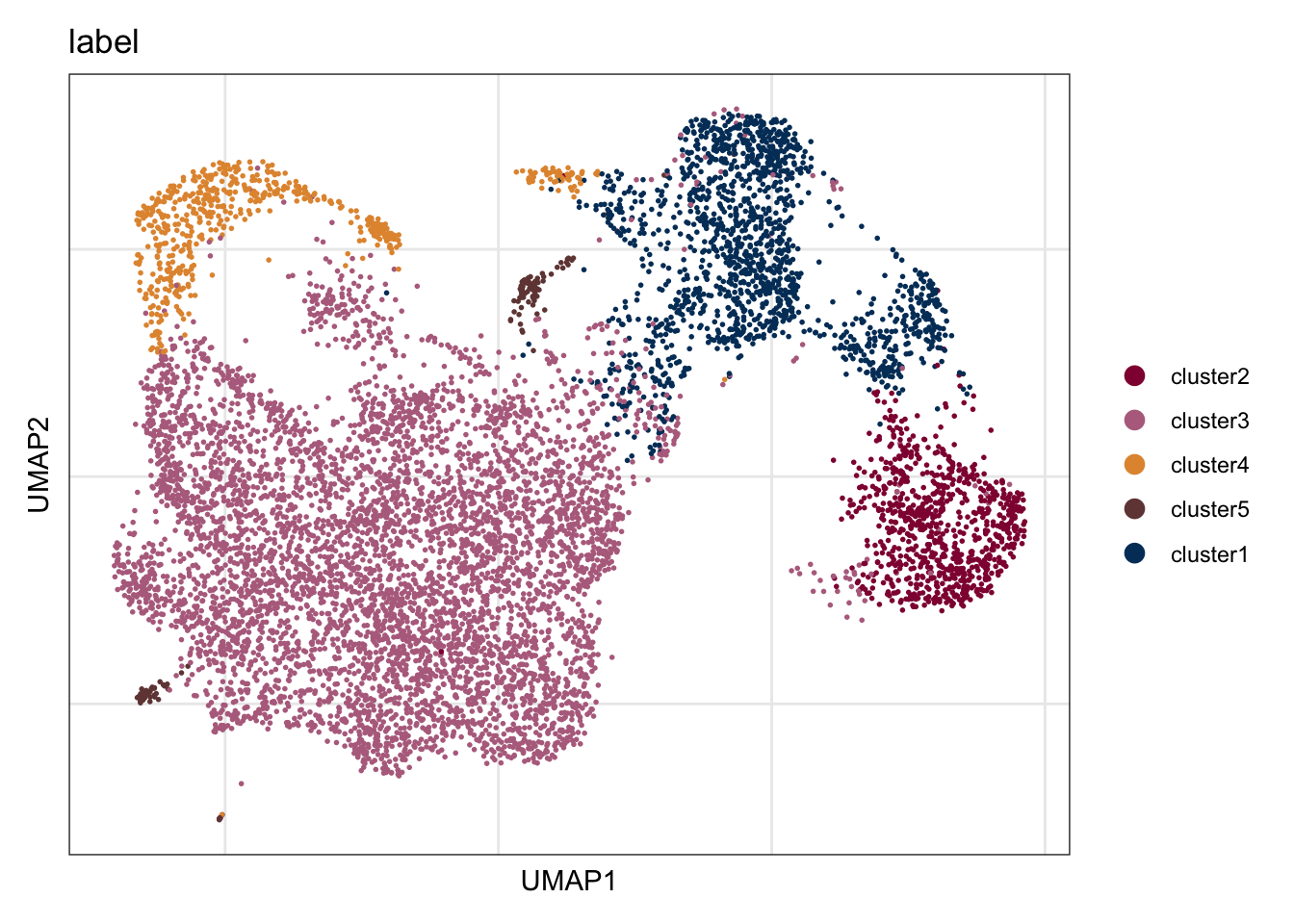
DimPlot(seuratE18EYFPv2.int, reduction = "umap", group.by = "label", pt.size=0.5,
        cols = colLab, shuffle = T)+
  theme_void()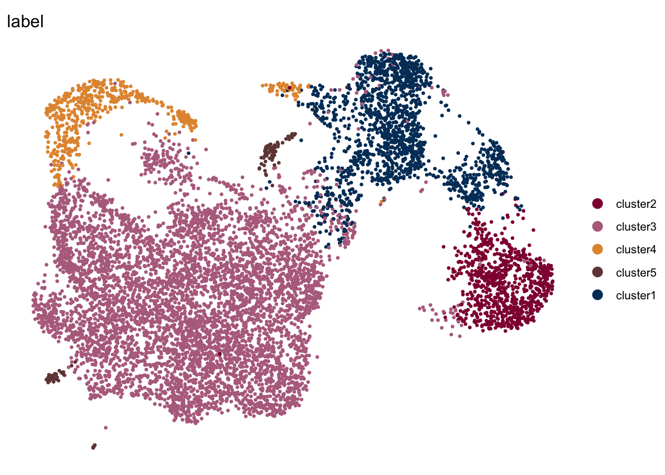
DimPlot(seuratE18EYFPv2.int, reduction = "umap", group.by = "label", pt.size=0.5,
        cols = colLab, shuffle = T)+
  theme_void() +
theme(legend.position = "none") 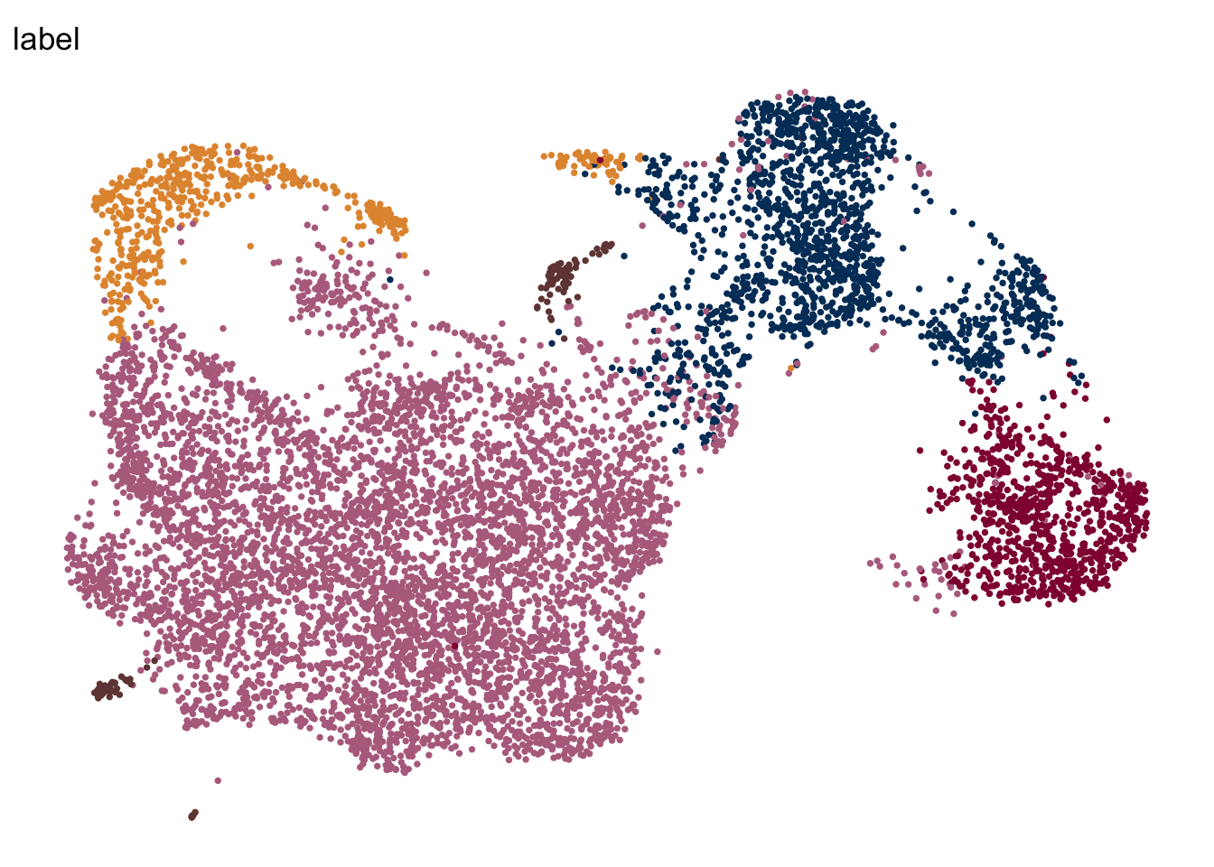
dotplot marker E18 EYFP+ fil
seurat_markers <- data.frame(gene=c("Vcam1", "Icam1",
                                    "Cxcl13", "Ccl19", "Ccl21a","Tnfsf11", "Grem1","Ifitm1","Cxcl1","Ifitm3","Ccl2","Nfkbia","Des",
                                    "Mfap5","Cdkn1c","Akap12","Anxa2","Lox","Gsn","Basp1","Fndc1","Sparc","Col1a1","Fbn2","Nr4a1","Fbln1","Cd34","Pi16",
                                    "Fbln5","Tm4sf1", "Ntrk3", "Fhl1", "Rgs7bp", "Adamts2", "Mpped2", "Ramp1", "Pdgfrl", "Eln", "Hspb2","Mgp", "Actg2","Acta2", "Myh11", "Mcam", "Mki67", "Ccna2", "Cdca8", "Prc1", "Aurkb"))

genes <- data.frame(geneID=rownames(seuratE18EYFPv2.int)) %>%
  mutate(gene=gsub(".*\\.", "",  geneID))

markerAll <- seurat_markers %>% left_join(., genes, by="gene")


## Dotplot all
Idents(seuratE18EYFPv2.int) <- seuratE18EYFPv2.int$label

DotPlot(seuratE18EYFPv2.int, assay="RNA", features = rev(markerAll$geneID), scale =T,
        cluster.idents = F) +
  scale_color_viridis_c() +
  coord_flip() +
  theme(axis.text.x = element_text(angle = 90, hjust = 1)) +
  scale_x_discrete(breaks=rev(markerAll$geneID), labels=rev(markerAll$gene)) +
  xlab("") + ylab("")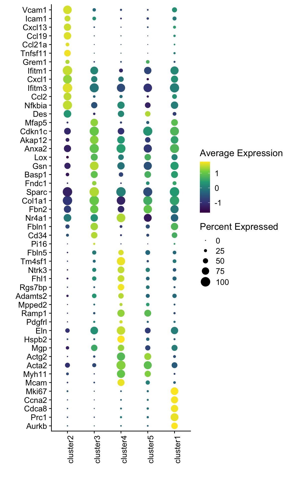
###signatures #### convert to sce
## convert seurat object to sce object
## exteract logcounts
logcounts <- GetAssayData(seuratE18EYFPv2.int, assay = "RNA", slot = "data")
counts <- GetAssayData(seuratE18EYFPv2.int, assay = "RNA", slot = "counts")
## extract reduced dims from integrated assay
pca <- Embeddings(seuratE18EYFPv2.int, reduction = "pca")
umap <- Embeddings(seuratE18EYFPv2.int, reduction = "umap")
## create sce object
sce <- SingleCellExperiment(assays =list (
  counts = counts,
  logcounts = logcounts
),
colData = seuratE18EYFPv2.int@meta.data,
rowData = data.frame(gene_id = rownames(logcounts)),
reducedDims = SimpleList(
  PCA = pca,
  UMAP = umap
))

genes <- data.frame(geneID=rownames(sce)) %>% mutate(gene=gsub(".*\\.", "", geneID))
pal = colorRampPalette(c("#053061", "#2166ac", "#f7f7f7", "#f4a582", "#b2183c", "#85122d"))
signatures
selGenes <- data.frame(gene=c("Cxcl13", "Ccl19", "Ccl21a","Tnfsf11", "Grem1"))
signGenes <- genes %>% dplyr::filter(gene %in% selGenes$gene)

##make a count matrix of signature genes
sceSub <- sce[which(rownames(sce) %in% signGenes$geneID),]
cntMat <- rowSums(t(as.matrix(
    sceSub@assays@data$logcounts)))/nrow(signGenes)
sceSub$sign <- cntMat
sceSub$sign2 <- sceSub$sign
sc <- scale_colour_gradientn(colours = pal(100), limits=c(0, 3))
sceSub$sign2[which(sceSub$sign > 3)] <- 3
##check max and min values
max(sceSub$sign)
[1] 2.88562min(sceSub$sign)[1] 0plotUMAP(sceSub, colour_by = "sign2", point_size = 1) + sc +
theme(legend.position = "none")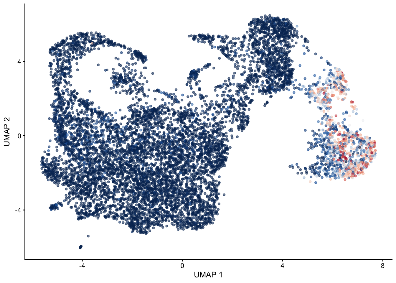
plotUMAP(sceSub, colour_by = "sign2", point_size = 1) + sc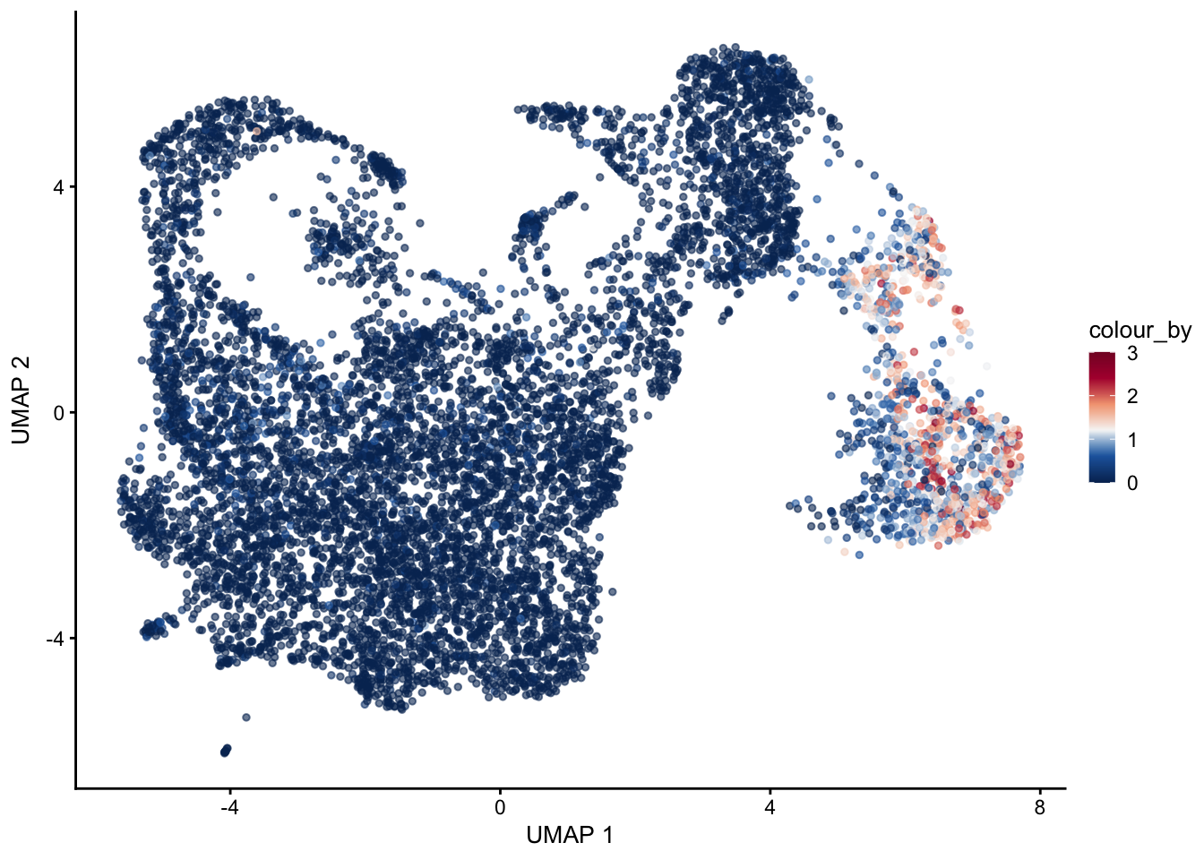
selGenes <- data.frame(gene=c("Mfap5","Gsn","Fndc1","Col1a1","Cd34"))
signGenes <- genes %>% dplyr::filter(gene %in% selGenes$gene)

##make a count matrix of signature genes
sceSub <- sce[which(rownames(sce) %in% signGenes$geneID),]
cntMat <- rowSums(t(as.matrix(
    sceSub@assays@data$logcounts)))/nrow(signGenes)
sceSub$sign <- cntMat
sceSub$sign2 <- sceSub$sign
sc <- scale_colour_gradientn(colours = pal(100), limits=c(0, 3))
sceSub$sign2[which(sceSub$sign > 3)] <- 3
##check max and min values
max(sceSub$sign)
[1] 3.469675min(sceSub$sign)[1] 0plotUMAP(sceSub, colour_by = "sign2", point_size = 1) + sc +
theme(legend.position = "none")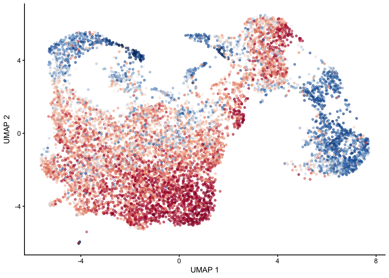
plotUMAP(sceSub, colour_by = "sign2", point_size = 1) + sc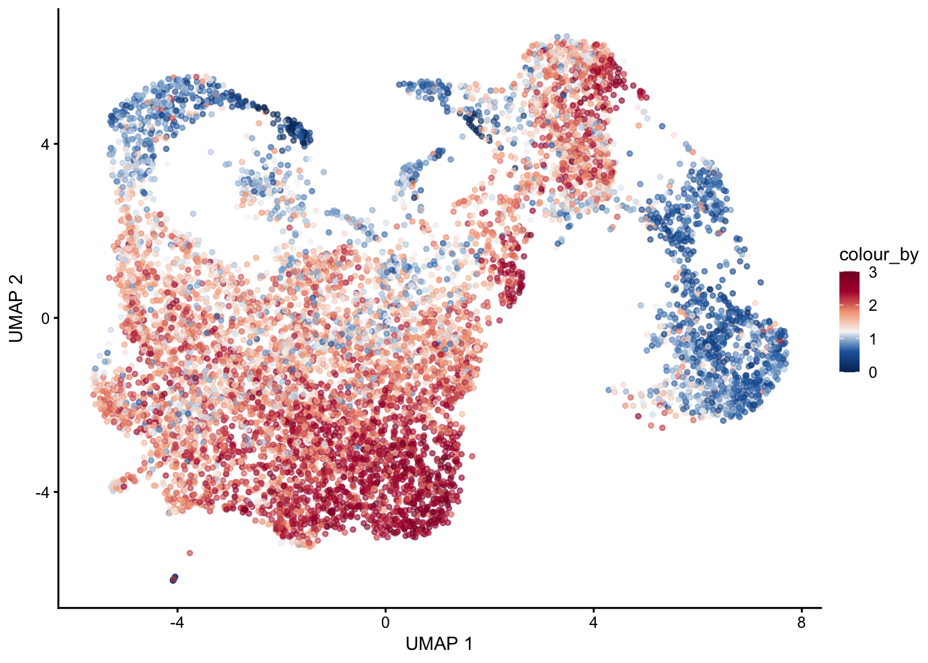
selGenes <- data.frame(gene=c("Fbln5","Eln","Actg2","Acta2","Myh11"))
signGenes <- genes %>% dplyr::filter(gene %in% selGenes$gene)

##make a count matrix of signature genes
sceSub <- sce[which(rownames(sce) %in% signGenes$geneID),]
cntMat <- rowSums(t(as.matrix(
    sceSub@assays@data$logcounts)))/nrow(signGenes)
sceSub$sign <- cntMat
sceSub$sign2 <- sceSub$sign
sc <- scale_colour_gradientn(colours = pal(100), limits=c(0, 3))
sceSub$sign2[which(sceSub$sign > 3)] <- 3
##check max and min values
max(sceSub$sign)
[1] 4.23627plotUMAP(sceSub, colour_by = "sign2", point_size = 1) + sc +
theme(legend.position = "none")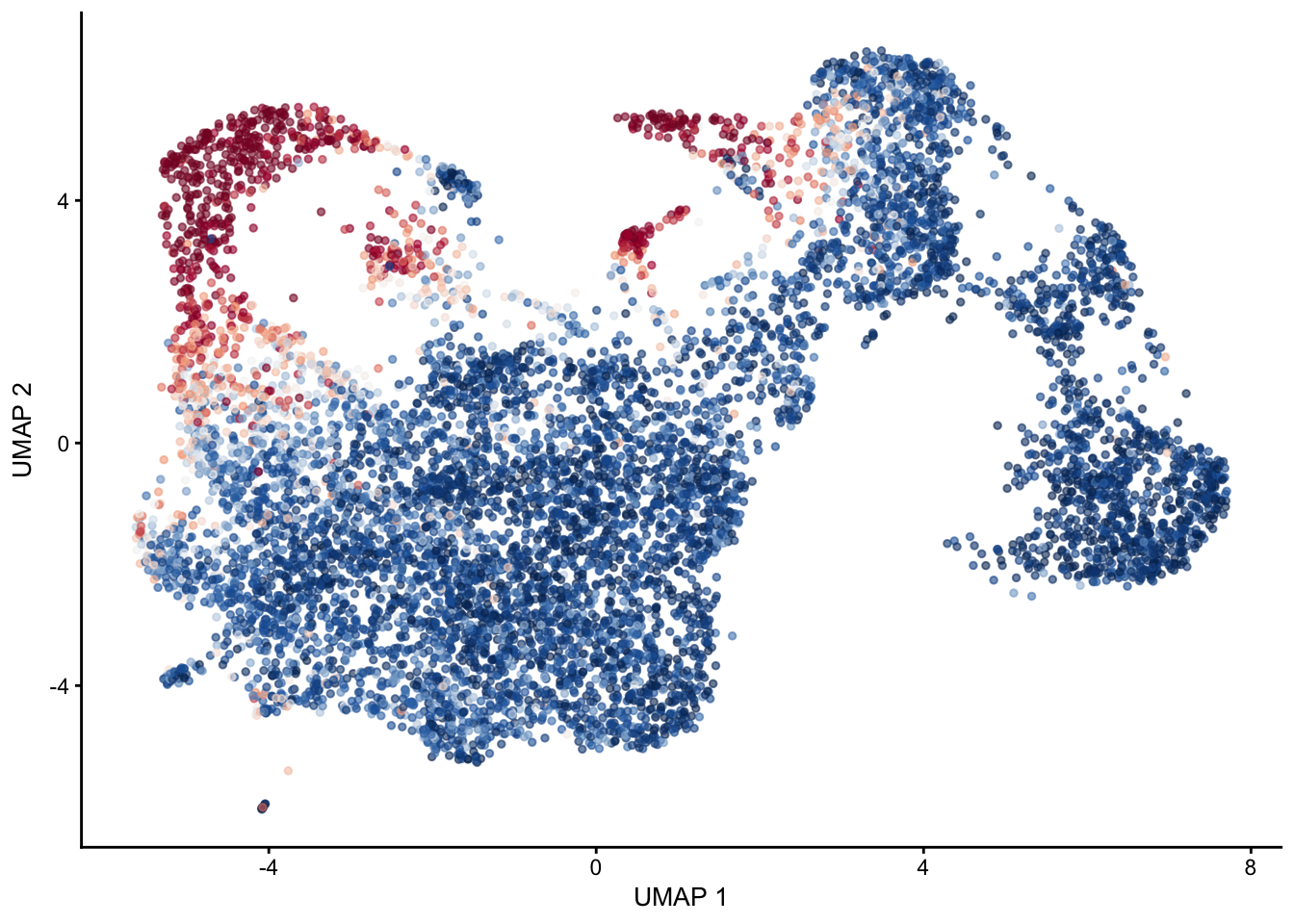
plotUMAP(sceSub, colour_by = "sign2", point_size = 1) + sc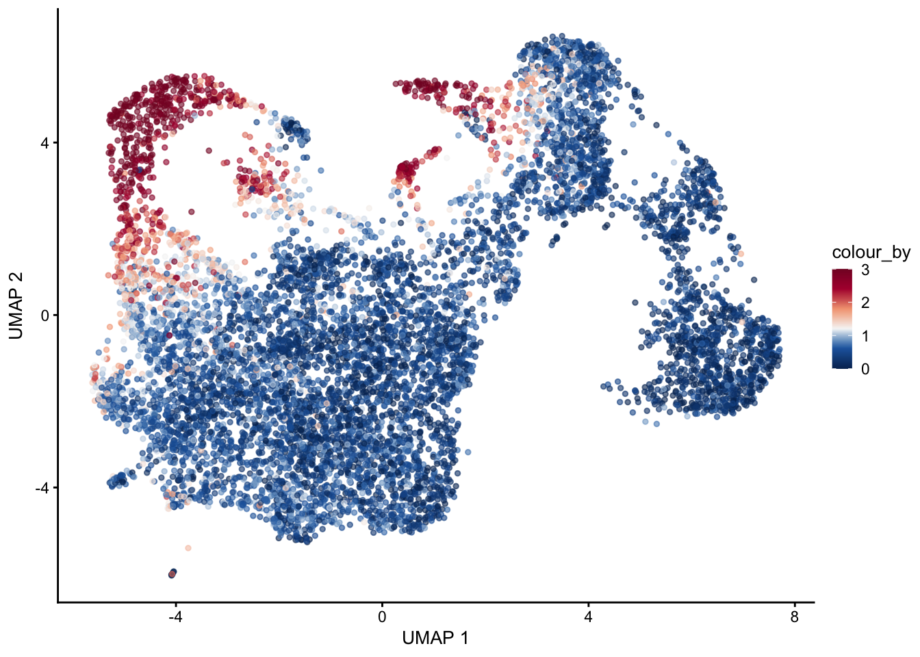
plot signature 3/4 combined
selGenes <- data.frame(gene=c("Fbln5","Eln","Actg2","Acta2","Myh11","Mfap5","Gsn","Fndc1","Col1a1","Cd34"))
signGenes <- genes %>% dplyr::filter(gene %in% selGenes$gene)

##make a count matrix of signature genes
sceSub <- sce[which(rownames(sce) %in% signGenes$geneID),]
cntMat <- rowSums(t(as.matrix(
    sceSub@assays@data$logcounts)))/nrow(signGenes)
sceSub$sign <- cntMat
sceSub$sign2 <- sceSub$sign
sc <- scale_colour_gradientn(colours = pal(100), limits=c(0, 2.5))
sceSub$sign2[which(sceSub$sign > 2.5)] <- 2.5
##check max and min values
max(sceSub$sign)
[1] 2.747664plotUMAP(sceSub, colour_by = "sign2", point_size = 1) + sc +
theme(legend.position = "none")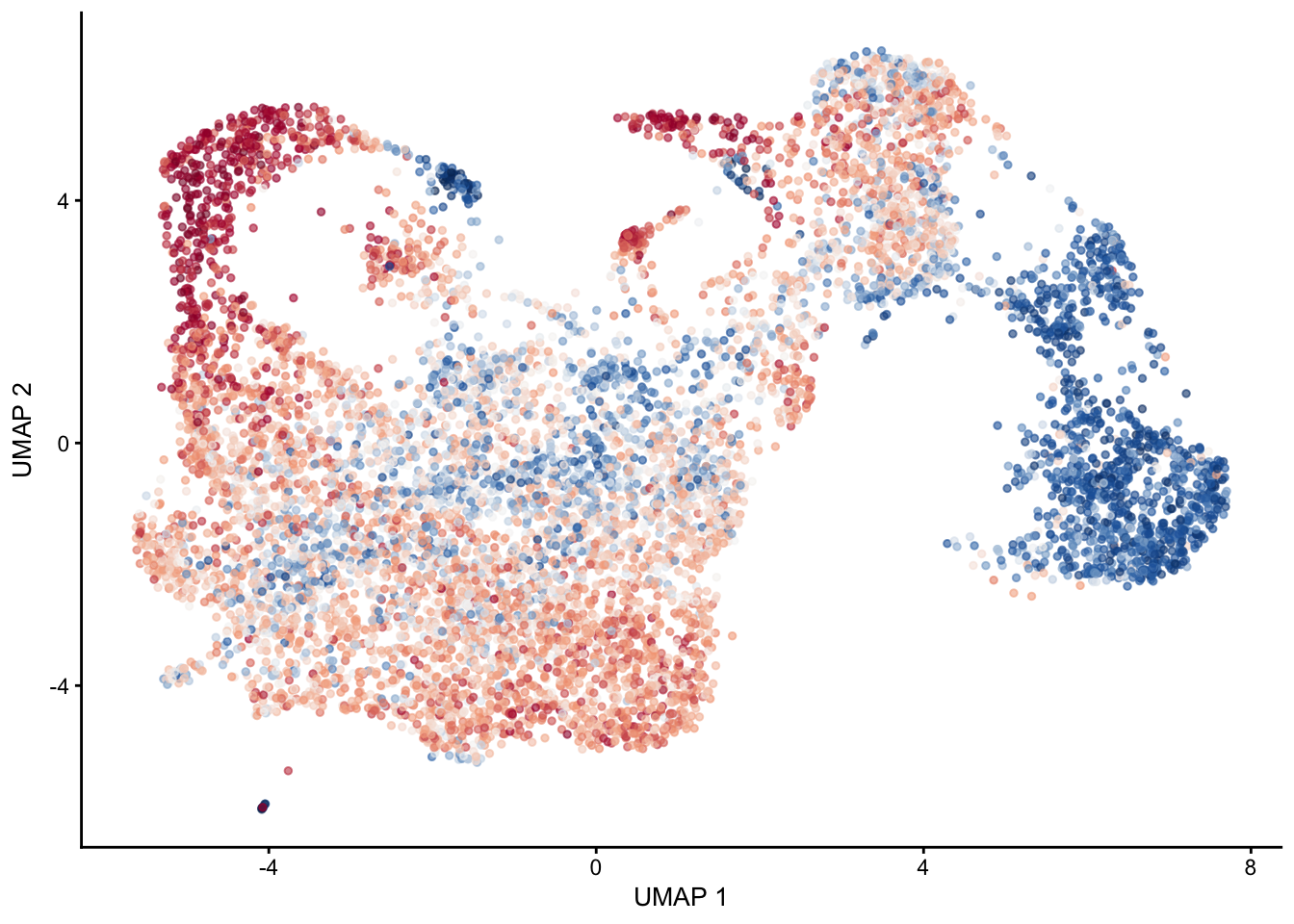
plotUMAP(sceSub, colour_by = "sign2", point_size = 1) + sc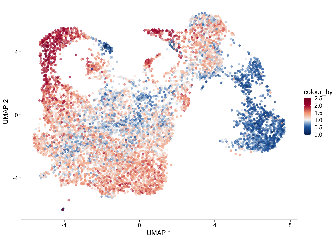
selGenes <- data.frame(gene=c("Mki67", "Ccna2", "Cdca8", "Prc1", "Aurkb"))
signGenes <- genes %>% dplyr::filter(gene %in% selGenes$gene)

##make a count matrix of signature genes
sceSub <- sce[which(rownames(sce) %in% signGenes$geneID),]
cntMat <- rowSums(t(as.matrix(
    sceSub@assays@data$logcounts)))/nrow(signGenes)
sceSub$sign <- cntMat
sceSub$sign2 <- sceSub$sign
sc <- scale_colour_gradientn(colours = pal(100), limits=c(0, 2))
sceSub$sign2[which(sceSub$sign > 2)] <- 2
##check max and min values
max(sceSub$sign)
[1] 2.106508plotUMAP(sceSub, colour_by = "sign2", point_size = 1) + sc +
theme(legend.position = "none")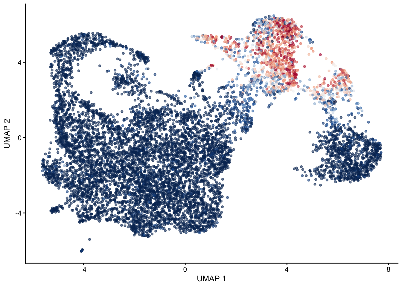
plotUMAP(sceSub, colour_by = "sign2", point_size = 1) + sc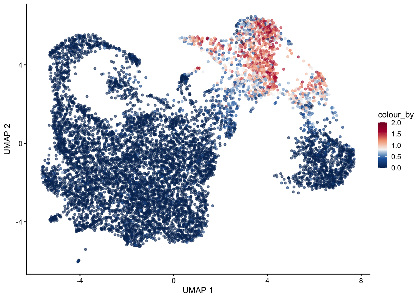
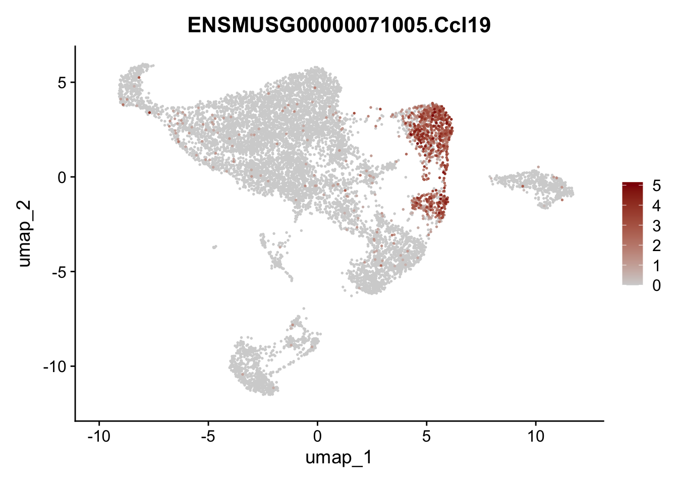
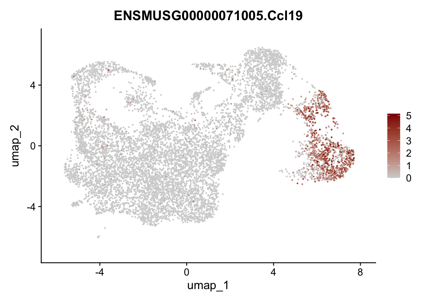
featrue Ccl19
genes <- data.frame(gene=rownames(seuratE18EYFPv2.int)) %>%
    mutate(geneID=gsub("^.*\\.", "", gene))

selGenes <- data.frame(geneID=c("Ccl19")) %>%
  left_join(., genes, by = "geneID")

pList <- sapply(selGenes$gene, function(x){
  p <- FeaturePlot(seuratE18EYFPv2.int, reduction = "umap",
            features = x,
            cols=c("lightgrey","darkred"),
            order = FALSE)+
  theme(legend.position="right")
  plot(p)
})
subset Ccl19 positive cells
seuratCcl19 <- subset(seuratE18EYFPv2.int, ENSMUSG00000071005.Ccl19 > 0)
table(seuratE18EYFPv2.int$orig.ident)
8787 table(seuratCcl19$orig.ident)
1023 rerun Ccl19 positive only
## rerun seurat
DefaultAssay(object = seuratCcl19) <- "integrated"
seuratCcl19 <- ScaleData(object = seuratCcl19, verbose = FALSE,
                         features = rownames(seuratCcl19))
seuratCcl19 <- RunPCA(object = seuratCcl19, npcs = 20, verbose = FALSE)
seuratCcl19 <- RunTSNE(object = seuratCcl19, recuction = "pca", dims = 1:20)
seuratCcl19 <- RunUMAP(object = seuratCcl19, recuction = "pca", dims = 1:20)

seuratCcl19 <- FindNeighbors(object = seuratCcl19, reduction = "pca", dims = 1:20)
res <- c(0.1, 0.6, 0.8, 0.4, 0.25)
for (i in 1:length(res)){
  seuratCcl19 <- FindClusters(object = seuratCcl19, resolution = res[i],
                              random.seed = 1234)
}
Modularity Optimizer version 1.3.0 by Ludo Waltman and Nees Jan van Eck
Number of nodes: 1023
Number of edges: 35579
Running Louvain algorithm...
Maximum modularity in 10 random starts: 0.9211
Number of communities: 2
Elapsed time: 0 seconds
Modularity Optimizer version 1.3.0 by Ludo Waltman and Nees Jan van Eck
Number of nodes: 1023
Number of edges: 35579
Running Louvain algorithm...
Maximum modularity in 10 random starts: 0.7329
Number of communities: 5
Elapsed time: 0 seconds
Modularity Optimizer version 1.3.0 by Ludo Waltman and Nees Jan van Eck
Number of nodes: 1023
Number of edges: 35579
Running Louvain algorithm...
Maximum modularity in 10 random starts: 0.6914
Number of communities: 5
Elapsed time: 0 seconds
Modularity Optimizer version 1.3.0 by Ludo Waltman and Nees Jan van Eck
Number of nodes: 1023
Number of edges: 35579
Running Louvain algorithm...
Maximum modularity in 10 random starts: 0.7876
Number of communities: 4
Elapsed time: 0 seconds
Modularity Optimizer version 1.3.0 by Ludo Waltman and Nees Jan van Eck
Number of nodes: 1023
Number of edges: 35579
Running Louvain algorithm...
Maximum modularity in 10 random starts: 0.8482
Number of communities: 3
Elapsed time: 0 secondsDefaultAssay(object = seuratCcl19) <- "RNA"
Idents(seuratCcl19) <- seuratCcl19$integrated_snn_res.0.25
colPal <- c("#DAF7A6", "#FFC300", "#FF5733", "#C70039", "#900C3F", "#b66e8d",
"#61a4ba", "#6178ba", "#54a87f", "#25328a", "#b6856e",
"#ba6161", "#20714a", "#0073C2FF", "#EFC000FF", "#868686FF",
"#CD534CFF","#7AA6DCFF", "#003C67FF", "#8F7700FF", "#3B3B3BFF",
"#A73030FF", "#4A6990FF")[1:length(unique(seuratCcl19$integrated_snn_res.0.25))]
names(colPal) <- unique(seuratCcl19$integrated_snn_res.0.25)dimplots Ccl19+ cells
clustering
DimPlot(seuratCcl19, reduction = "umap",
        label = T, shuffle = T, cols = colPal) +
  theme_bw() +
  theme(axis.text = element_blank(), axis.ticks = element_blank(),
        panel.grid.minor = element_blank()) +
  xlab("umap1") +
  ylab("umap2")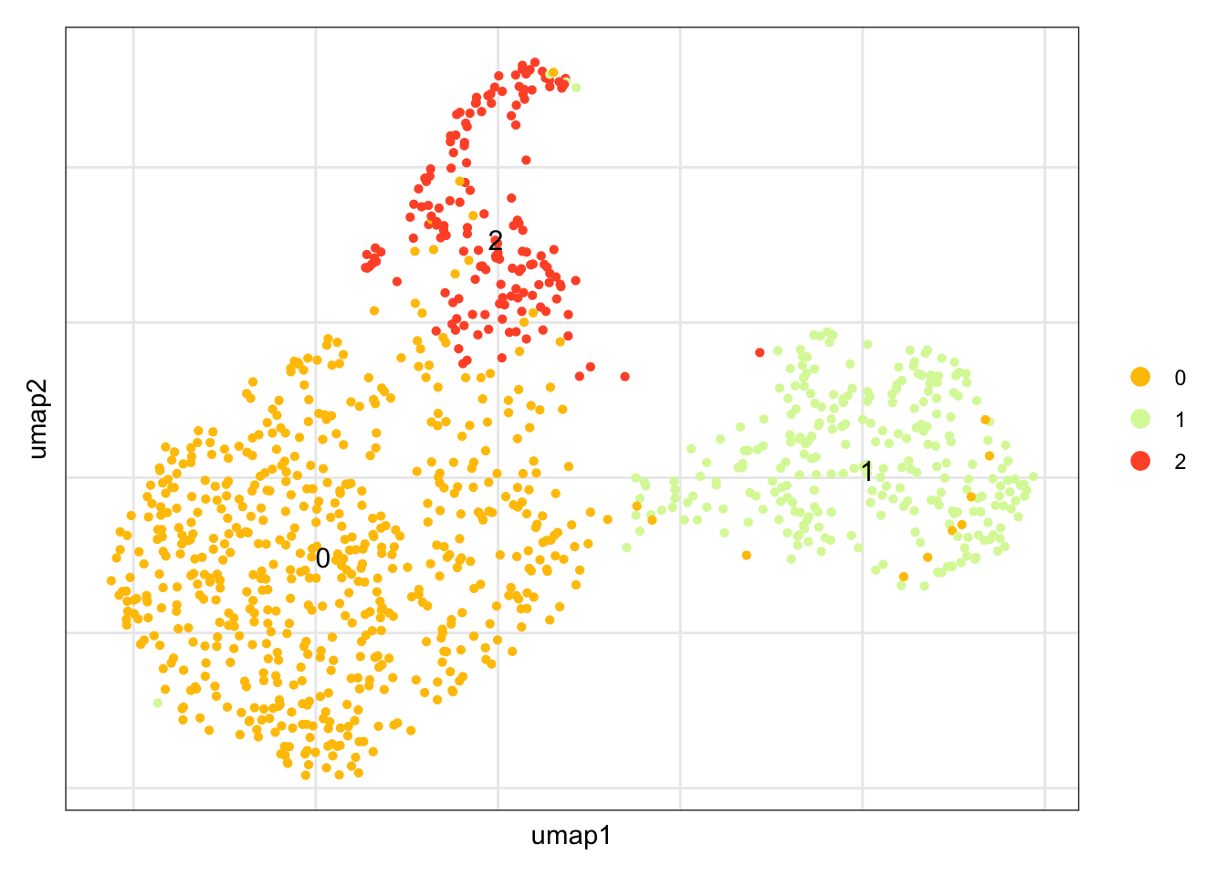
assign label Ccl19+ cells
seuratCcl19$label <- "label"
seuratCcl19$label[which(seuratCcl19$integrated_snn_res.0.25 == "0")] <- "cluster2"
seuratCcl19$label[which(seuratCcl19$integrated_snn_res.0.25 == "1")] <- "cluster1"
seuratCcl19$label[which(seuratCcl19$integrated_snn_res.0.25 == "2")] <- "cluster3"
table(seuratCcl19$label)
cluster1 cluster2 cluster3
     266      597      160
##order
seuratCcl19$label <- factor(seuratCcl19$label, levels = c("cluster2", "cluster3","cluster1"))
table(seuratCcl19$label)
cluster2 cluster3 cluster1
     597      160      266
colLab <- c("#900C3F","#b66e8d", "#003C67FF")
names(colLab) <- c("cluster2", "cluster3", "cluster1")label
DimPlot(seuratCcl19, reduction = "umap", group.by = "label", cols = colLab)+
  theme_bw() +
  theme(axis.text = element_blank(), axis.ticks = element_blank(),
        panel.grid.minor = element_blank()) +
  xlab("UMAP1") +
  ylab("UMAP2")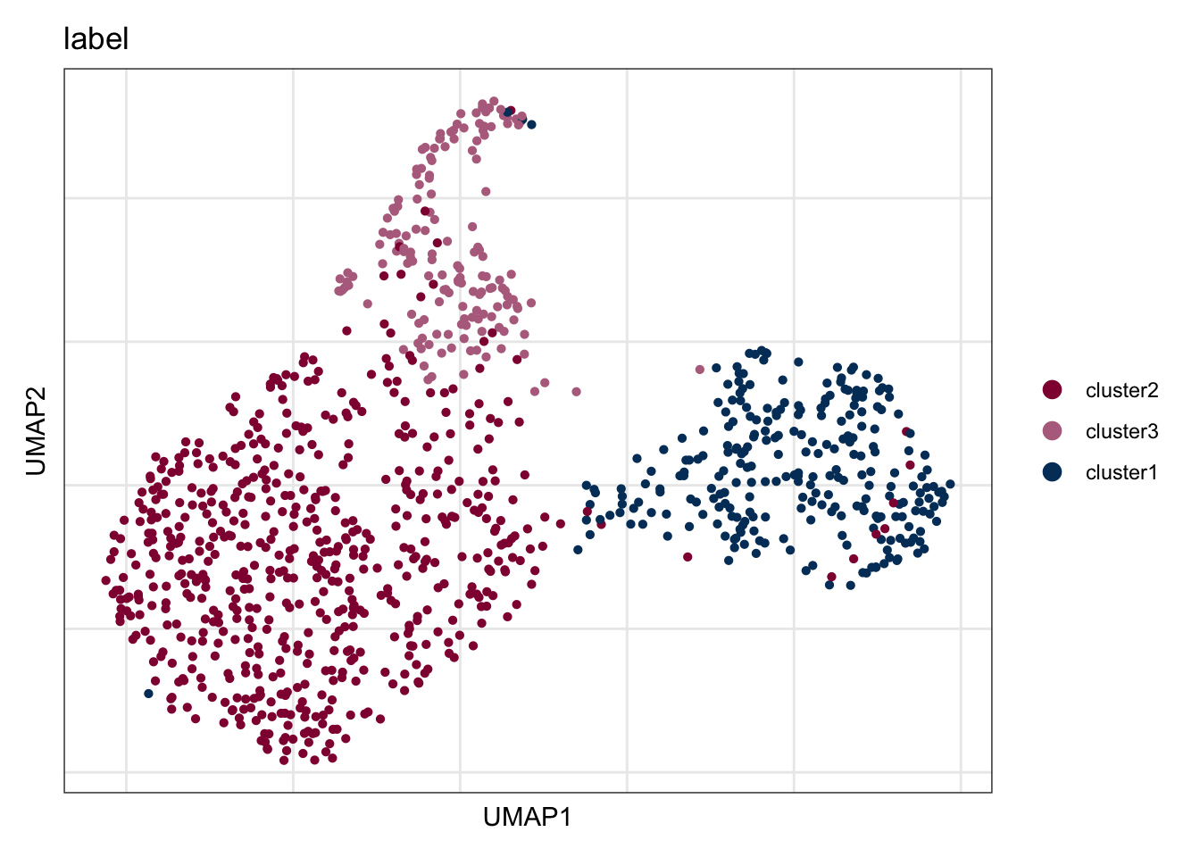
DimPlot(seuratCcl19, reduction = "umap", group.by = "label", pt.size=0.5,
        cols = colLab, shuffle = T)+
  theme_void()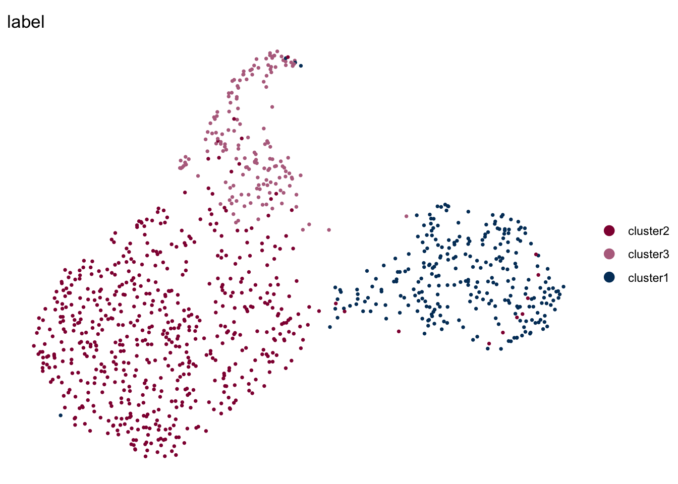
DimPlot(seuratCcl19, reduction = "umap", group.by = "label", pt.size=0.5,
        cols = colLab, shuffle = T)+
  theme_void() +
theme(legend.position = "none") 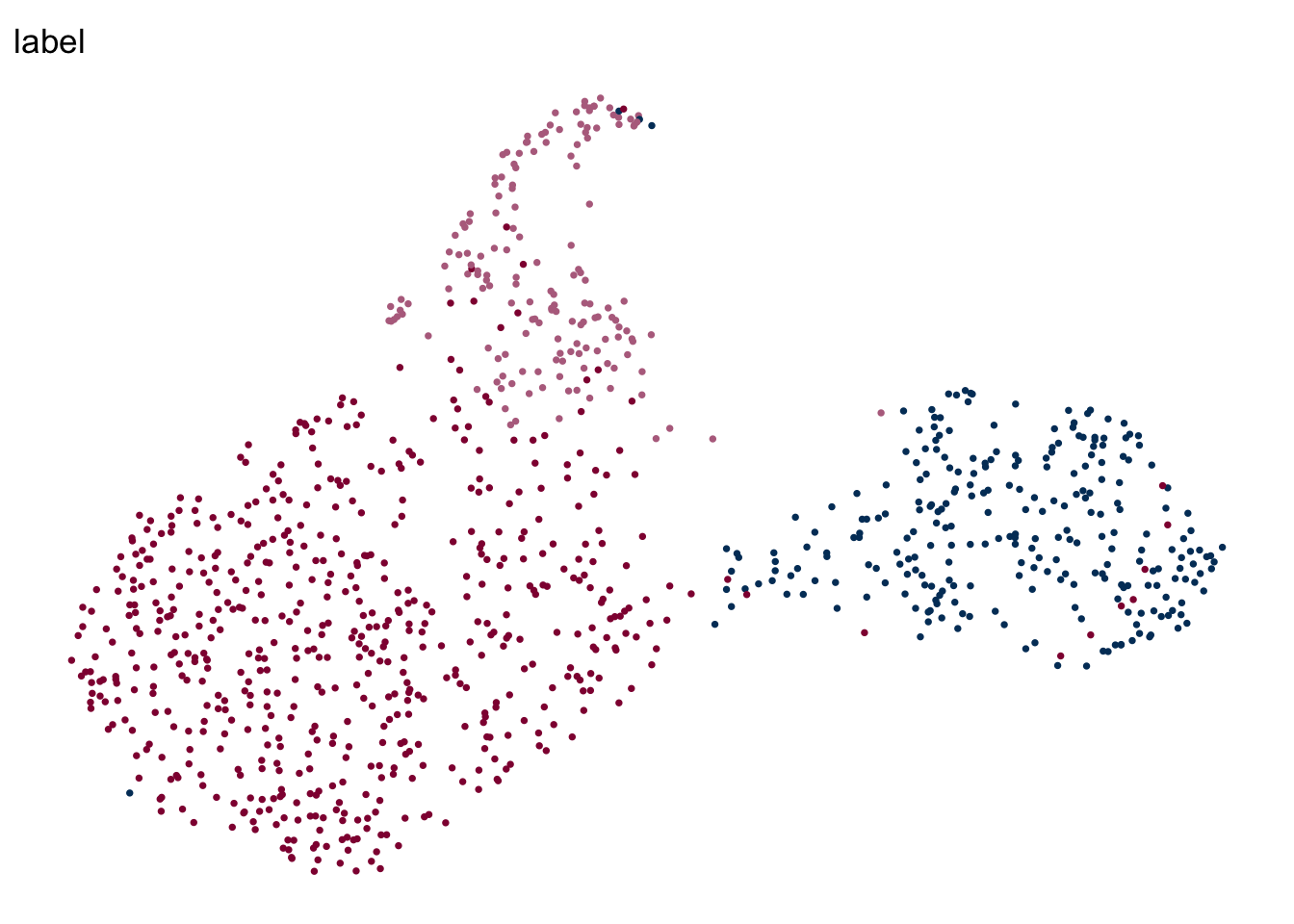
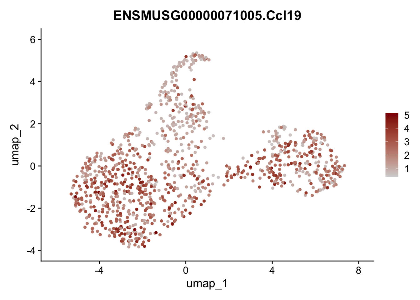
featrue plot Ccl19
genes <- data.frame(gene=rownames(seuratCcl19)) %>%
    mutate(geneID=gsub("^.*\\.", "", gene))

selGenes <- data.frame(geneID=c("Ccl19")) %>%
  left_join(., genes, by = "geneID")

pList <- sapply(selGenes$gene, function(x){
  p <- FeaturePlot(seuratCcl19, reduction = "umap",
            features = x,
            cols=c("lightgrey","darkred"),
            order = FALSE)+
  theme(legend.position="right")
  plot(p)
})
signatures Ccl19+ cells
##convert seurat object to sce object
##exteract logcounts
logcounts <- GetAssayData(seuratCcl19, assay = "RNA", slot = "data")
counts <- GetAssayData(seuratCcl19, assay = "RNA", slot = "counts")
##extract reduced dims from integrated assay
pca <- Embeddings(seuratCcl19, reduction = "pca")
umap <- Embeddings(seuratCcl19, reduction = "umap")
##create sce object
sce <- SingleCellExperiment(assays =list (
  counts = counts,
  logcounts = logcounts
),
colData = seuratCcl19@meta.data,
rowData = data.frame(gene_id = rownames(logcounts)),
reducedDims = SimpleList(
  PCA = pca,
  UMAP = umap
))

genes <- data.frame(geneID=rownames(sce)) %>% mutate(gene=gsub(".*\\.", "", geneID))
pal = colorRampPalette(c("#053061", "#2166ac", "#f7f7f7", "#f4a582", "#b2183c", "#85122d"))
selGenes <- data.frame(gene=c("Cxcl13","Ccl19", "Ccl21a","Tnfsf11", "Grem1"))
signGenes <- genes %>% dplyr::filter(gene %in% selGenes$gene)
##make a count matrix of signature genes
sceSub <- sce[which(rownames(sce) %in% signGenes$geneID),]
cntMat <- rowSums(t(as.matrix(
sceSub@assays@data$logcounts)))/nrow(signGenes)
sceSub$sign <- cntMat
sceSub$sign2 <- sceSub$sign
sc <- scale_colour_gradientn(colours = pal(100), limits=c(0, 2.5))
sceSub$sign2[which(sceSub$sign > 2.5)] <- 2.5
sceSub$sign2[which(sceSub$sign < 0)] <- 0
##check max and min values
max(sceSub$sign)[1] 2.88562min(sceSub$sign)[1] 0.1052551plotUMAP(sceSub, colour_by = "sign2", point_size = 1) + sc +
theme(legend.position = "none")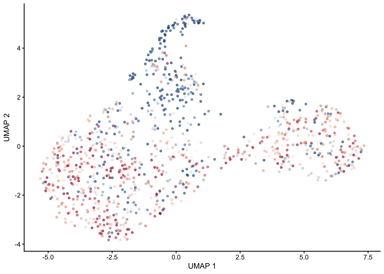
plotUMAP(sceSub, colour_by = "sign2", point_size = 1) + sc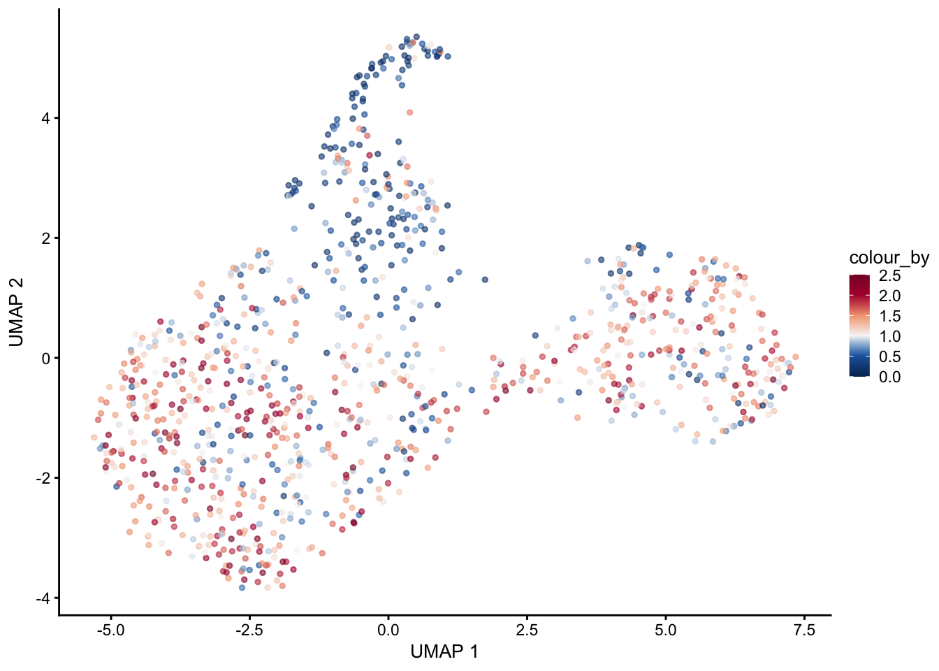
selGenes <- data.frame(gene=c("Fbln5","Eln","Actg2","Acta2","Myh11","Mfap5","Gsn","Fndc1","Col1a1","Cd34"))
signGenes <- genes %>% dplyr::filter(gene %in% selGenes$gene)

##make a count matrix of signature genes
sceSub <- sce[which(rownames(sce) %in% signGenes$geneID),]
cntMat <- rowSums(t(as.matrix(
    sceSub@assays@data$logcounts)))/nrow(signGenes)
sceSub$sign <- cntMat
sceSub$sign2 <- sceSub$sign
sc <- scale_colour_gradientn(colours = pal(100), limits=c(0, 2.5))
sceSub$sign2[which(sceSub$sign > 2.5)] <- 2.5
sceSub$sign2[which(sceSub$sign < 0)] <- 0
##check max and min values
max(sceSub$sign)
[1] 2.532537min(sceSub$sign)[1] 0plotUMAP(sceSub, colour_by = "sign2", point_size = 1) + sc +
theme(legend.position = "none")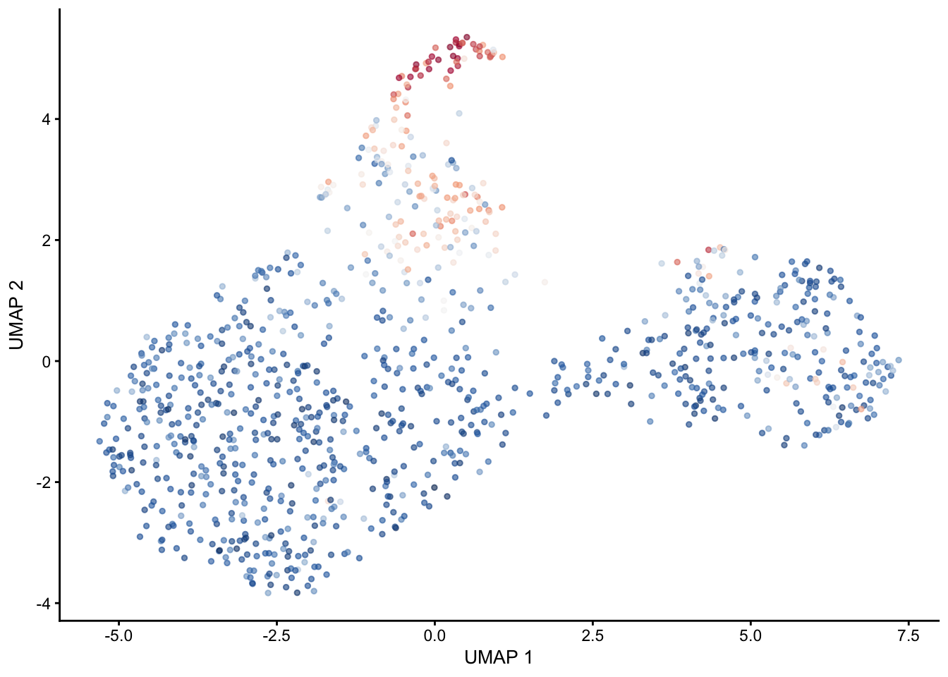
plotUMAP(sceSub, colour_by = "sign2", point_size = 1) + sc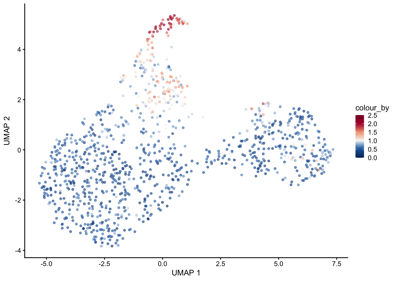
selGenes <- data.frame(gene=c("Mki67", "Ccna2", "Cdca8", "Prc1", "Aurkb"))
signGenes <- genes %>% dplyr::filter(gene %in% selGenes$gene)

##make a count matrix of signature genes
sceSub <- sce[which(rownames(sce) %in% signGenes$geneID),]
cntMat <- rowSums(t(as.matrix(
    sceSub@assays@data$logcounts)))/nrow(signGenes)
sceSub$sign <- cntMat
sceSub$sign2 <- sceSub$sign
sc <- scale_colour_gradientn(colours = pal(100), limits=c(0, 2))
sceSub$sign2[which(sceSub$sign > 2)] <- 2
sceSub$sign2[which(sceSub$sign < 0)] <- 0
##check max and min values
max(sceSub$sign)
[1] 1.967789min(sceSub$sign)[1] 0plotUMAP(sceSub, colour_by = "sign2", point_size = 1) + sc +
theme(legend.position = "none")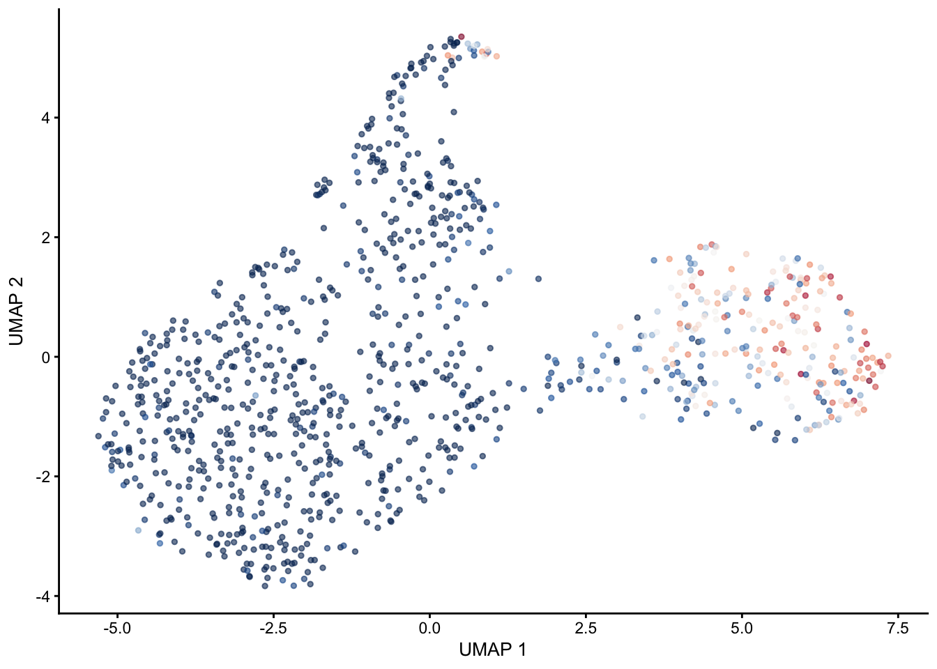
plotUMAP(sceSub, colour_by = "sign2", point_size = 1) + sc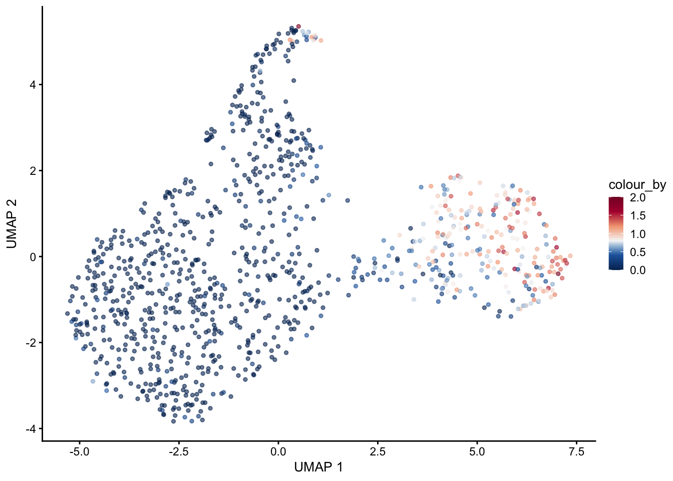
session info
date()[1] "Tue Jul 15 14:49:20 2025"sessionInfo()R version 4.4.0 (2024-04-24)
Platform: x86_64-apple-darwin20
Running under: macOS Ventura 13.7.6
Matrix products: default
BLAS: /Library/Frameworks/R.framework/Versions/4.4-x86_64/Resources/lib/libRblas.0.dylib
LAPACK: /Library/Frameworks/R.framework/Versions/4.4-x86_64/Resources/lib/libRlapack.dylib; LAPACK version 3.12.0
locale:
[1] en_US.UTF-8/en_US.UTF-8/en_US.UTF-8/C/en_US.UTF-8/en_US.UTF-8
time zone: Europe/Zurich
tzcode source: internal
attached base packages:
[1] grid stats4 stats graphics grDevices utils datasets methods base
other attached packages:
[1] future_1.58.0 here_1.0.1 slingshot_2.12.0
[4] TrajectoryUtils_1.12.0 princurve_2.1.6 NCmisc_1.2.0
[7] VennDiagram_1.7.3 futile.logger_1.4.3 ggupset_0.4.1
[10] gridExtra_2.3 DOSE_3.30.5 enrichplot_1.24.4
[13] msigdbr_24.1.0 org.Mm.eg.db_3.19.1 AnnotationDbi_1.66.0
[16] clusterProfiler_4.12.6 multtest_2.60.0 metap_1.12
[19] scater_1.32.1 scuttle_1.14.0 destiny_3.18.0
[22] circlize_0.4.16 muscat_1.18.0 viridis_0.6.5
[25] viridisLite_0.4.2 lubridate_1.9.4 forcats_1.0.0
[28] stringr_1.5.1 purrr_1.0.4 readr_2.1.5
[31] tidyr_1.3.1 tibble_3.2.1 tidyverse_2.0.0
[34] dplyr_1.1.4 SingleCellExperiment_1.26.0 SummarizedExperiment_1.34.0
[37] Biobase_2.64.0 GenomicRanges_1.56.2 GenomeInfoDb_1.40.1
[40] IRanges_2.38.1 S4Vectors_0.42.1 BiocGenerics_0.50.0
[43] MatrixGenerics_1.16.0 matrixStats_1.5.0 pheatmap_1.0.13
[46] ggpubr_0.6.0 ggplot2_3.5.2 Seurat_5.3.0
[49] SeuratObject_5.1.0 sp_2.2-0 runSeurat3_0.1.0
[52] ExploreSCdataSeurat3_0.1.0
loaded via a namespace (and not attached):
[1] igraph_2.1.4 ica_1.0-3 plotly_4.10.4
[4] Formula_1.2-5 zlibbioc_1.50.0 tidyselect_1.2.1
[7] bit_4.6.0 doParallel_1.0.17 clue_0.3-66
[10] lattice_0.22-7 rjson_0.2.23 blob_1.2.4
[13] S4Arrays_1.4.1 pbkrtest_0.5.4 parallel_4.4.0
[16] png_0.1-8 plotrix_3.8-4 cli_3.6.5
[19] ggplotify_0.1.2 goftest_1.2-3 VIM_6.2.2
[22] variancePartition_1.34.0 BiocNeighbors_1.22.0 shadowtext_0.1.4
[25] uwot_0.2.3 curl_6.2.3 tidytree_0.4.6
[28] mime_0.13 evaluate_1.0.3 ComplexHeatmap_2.20.0
[31] stringi_1.8.7 backports_1.5.0 lmerTest_3.1-3
[34] qqconf_1.3.2 httpuv_1.6.16 magrittr_2.0.3
[37] rappdirs_0.3.3 splines_4.4.0 ggraph_2.2.1
[40] sctransform_0.4.2 ggbeeswarm_0.7.2 DBI_1.2.3
[43] jquerylib_0.1.4 smoother_1.3 withr_3.0.2
[46] git2r_0.36.2 corpcor_1.6.10 reformulas_0.4.1
[49] class_7.3-23 rprojroot_2.0.4 lmtest_0.9-40
[52] tidygraph_1.3.1 formatR_1.14 colourpicker_1.3.0
[55] htmlwidgets_1.6.4 fs_1.6.6 ggrepel_0.9.6
[58] labeling_0.4.3 fANCOVA_0.6-1 SparseArray_1.4.8
[61] DESeq2_1.44.0 ranger_0.17.0 DEoptimR_1.1-3-1
[64] reticulate_1.42.0 hexbin_1.28.5 zoo_1.8-14
[67] XVector_0.44.0 knitr_1.50 ggplot.multistats_1.0.1
[70] UCSC.utils_1.0.0 RhpcBLASctl_0.23-42 timechange_0.3.0
[73] foreach_1.5.2 patchwork_1.3.0 caTools_1.18.3
[76] data.table_1.17.4 ggtree_3.12.0 R.oo_1.27.1
[79] RSpectra_0.16-2 irlba_2.3.5.1 fastDummies_1.7.5
[82] gridGraphics_0.5-1 lazyeval_0.2.2 yaml_2.3.10
[85] survival_3.8-3 scattermore_1.2 crayon_1.5.3
[88] RcppAnnoy_0.0.22 RColorBrewer_1.1-3 progressr_0.15.1
[91] tweenr_2.0.3 later_1.4.2 ggridges_0.5.6
[94] codetools_0.2-20 GlobalOptions_0.1.2 aod_1.3.3
[97] KEGGREST_1.44.1 Rtsne_0.17 shape_1.4.6.1
[100] limma_3.60.6 pkgconfig_2.0.3 TMB_1.9.17
[103] spatstat.univar_3.1-3 mathjaxr_1.8-0 EnvStats_3.1.0
[106] aplot_0.2.5 scatterplot3d_0.3-44 ape_5.8-1
[109] spatstat.sparse_3.1-0 xtable_1.8-4 car_3.1-3
[112] plyr_1.8.9 httr_1.4.7 rbibutils_2.3
[115] tools_4.4.0 globals_0.18.0 beeswarm_0.4.0
[118] broom_1.0.8 nlme_3.1-168 lambda.r_1.2.4
[121] assertthat_0.2.1 lme4_1.1-37 digest_0.6.37
[124] numDeriv_2016.8-1.1 Matrix_1.7-3 farver_2.1.2
[127] tzdb_0.5.0 remaCor_0.0.18 reshape2_1.4.4
[130] yulab.utils_0.2.0 glue_1.8.0 cachem_1.1.0
[133] polyclip_1.10-7 generics_0.1.4 Biostrings_2.72.1
[136] mvtnorm_1.3-3 parallelly_1.45.0 mnormt_2.1.1
[139] statmod_1.5.0 RcppHNSW_0.6.0 ScaledMatrix_1.12.0
[142] carData_3.0-5 minqa_1.2.8 pbapply_1.7-2
[145] httr2_1.1.2 spam_2.11-1 gson_0.1.0
[148] graphlayouts_1.2.2 gtools_3.9.5 ggsignif_0.6.4
[151] RcppEigen_0.3.4.0.2 shiny_1.10.0 GenomeInfoDbData_1.2.12
[154] glmmTMB_1.1.11 R.utils_2.13.0 memoise_2.0.1
[157] rmarkdown_2.29 scales_1.4.0 R.methodsS3_1.8.2
[160] RANN_2.6.2 Cairo_1.6-2 spatstat.data_3.1-6
[163] rstudioapi_0.17.1 cluster_2.1.8.1 mutoss_0.1-13
[166] spatstat.utils_3.1-4 hms_1.1.3 fitdistrplus_1.2-2
[169] cowplot_1.1.3 colorspace_2.1-1 rlang_1.1.6
[172] DelayedMatrixStats_1.26.0 sparseMatrixStats_1.16.0 xts_0.14.1
[175] dotCall64_1.2 shinydashboard_0.7.3 ggforce_0.4.2
[178] laeken_0.5.3 mgcv_1.9-3 xfun_0.52
[181] e1071_1.7-16 TH.data_1.1-3 iterators_1.0.14
[184] abind_1.4-8 GOSemSim_2.30.2 treeio_1.28.0
[187] futile.options_1.0.1 bitops_1.0-9 Rdpack_2.6.4
[190] promises_1.3.3 scatterpie_0.2.4 RSQLite_2.4.0
[193] qvalue_2.36.0 sandwich_3.1-1 fgsea_1.30.0
[196] DelayedArray_0.30.1 proxy_0.4-27 GO.db_3.19.1
[199] compiler_4.4.0 prettyunits_1.2.0 boot_1.3-31
[202] beachmat_2.20.0 listenv_0.9.1 Rcpp_1.0.14
[205] edgeR_4.2.2 workflowr_1.7.1 BiocSingular_1.20.0
[208] tensor_1.5 MASS_7.3-65 progress_1.2.3
[211] BiocParallel_1.38.0 babelgene_22.9 spatstat.random_3.4-1
[214] R6_2.6.1 fastmap_1.2.0 multcomp_1.4-28
[217] fastmatch_1.1-6 rstatix_0.7.2 vipor_0.4.7
[220] TTR_0.24.4 ROCR_1.0-11 TFisher_0.2.0
[223] rsvd_1.0.5 vcd_1.4-13 nnet_7.3-20
[226] gtable_0.3.6 KernSmooth_2.23-26 miniUI_0.1.2
[229] deldir_2.0-4 htmltools_0.5.8.1 ggthemes_5.1.0
[232] bit64_4.6.0-1 spatstat.explore_3.4-3 lifecycle_1.0.4
[235] blme_1.0-6 nloptr_2.2.1 sass_0.4.10
[238] vctrs_0.6.5 robustbase_0.99-4-1 spatstat.geom_3.4-1
[241] sn_2.1.1 ggfun_0.1.8 future.apply_1.11.3
[244] bslib_0.9.0 pillar_1.10.2 gplots_3.2.0
[247] pcaMethods_1.96.0 locfit_1.5-9.12 jsonlite_2.0.0
[250] GetoptLong_1.0.5
sessionInfo()R version 4.4.0 (2024-04-24)
Platform: x86_64-apple-darwin20
Running under: macOS Ventura 13.7.6
Matrix products: default
BLAS: /Library/Frameworks/R.framework/Versions/4.4-x86_64/Resources/lib/libRblas.0.dylib
LAPACK: /Library/Frameworks/R.framework/Versions/4.4-x86_64/Resources/lib/libRlapack.dylib; LAPACK version 3.12.0
locale:
[1] en_US.UTF-8/en_US.UTF-8/en_US.UTF-8/C/en_US.UTF-8/en_US.UTF-8
time zone: Europe/Zurich
tzcode source: internal
attached base packages:
[1] grid stats4 stats graphics grDevices utils datasets methods base
other attached packages:
[1] future_1.58.0 here_1.0.1 slingshot_2.12.0
[4] TrajectoryUtils_1.12.0 princurve_2.1.6 NCmisc_1.2.0
[7] VennDiagram_1.7.3 futile.logger_1.4.3 ggupset_0.4.1
[10] gridExtra_2.3 DOSE_3.30.5 enrichplot_1.24.4
[13] msigdbr_24.1.0 org.Mm.eg.db_3.19.1 AnnotationDbi_1.66.0
[16] clusterProfiler_4.12.6 multtest_2.60.0 metap_1.12
[19] scater_1.32.1 scuttle_1.14.0 destiny_3.18.0
[22] circlize_0.4.16 muscat_1.18.0 viridis_0.6.5
[25] viridisLite_0.4.2 lubridate_1.9.4 forcats_1.0.0
[28] stringr_1.5.1 purrr_1.0.4 readr_2.1.5
[31] tidyr_1.3.1 tibble_3.2.1 tidyverse_2.0.0
[34] dplyr_1.1.4 SingleCellExperiment_1.26.0 SummarizedExperiment_1.34.0
[37] Biobase_2.64.0 GenomicRanges_1.56.2 GenomeInfoDb_1.40.1
[40] IRanges_2.38.1 S4Vectors_0.42.1 BiocGenerics_0.50.0
[43] MatrixGenerics_1.16.0 matrixStats_1.5.0 pheatmap_1.0.13
[46] ggpubr_0.6.0 ggplot2_3.5.2 Seurat_5.3.0
[49] SeuratObject_5.1.0 sp_2.2-0 runSeurat3_0.1.0
[52] ExploreSCdataSeurat3_0.1.0
loaded via a namespace (and not attached):
[1] igraph_2.1.4 ica_1.0-3 plotly_4.10.4
[4] Formula_1.2-5 zlibbioc_1.50.0 tidyselect_1.2.1
[7] bit_4.6.0 doParallel_1.0.17 clue_0.3-66
[10] lattice_0.22-7 rjson_0.2.23 blob_1.2.4
[13] S4Arrays_1.4.1 pbkrtest_0.5.4 parallel_4.4.0
[16] png_0.1-8 plotrix_3.8-4 cli_3.6.5
[19] ggplotify_0.1.2 goftest_1.2-3 VIM_6.2.2
[22] variancePartition_1.34.0 BiocNeighbors_1.22.0 shadowtext_0.1.4
[25] uwot_0.2.3 curl_6.2.3 tidytree_0.4.6
[28] mime_0.13 evaluate_1.0.3 ComplexHeatmap_2.20.0
[31] stringi_1.8.7 backports_1.5.0 lmerTest_3.1-3
[34] qqconf_1.3.2 httpuv_1.6.16 magrittr_2.0.3
[37] rappdirs_0.3.3 splines_4.4.0 ggraph_2.2.1
[40] sctransform_0.4.2 ggbeeswarm_0.7.2 DBI_1.2.3
[43] jquerylib_0.1.4 smoother_1.3 withr_3.0.2
[46] git2r_0.36.2 corpcor_1.6.10 reformulas_0.4.1
[49] class_7.3-23 rprojroot_2.0.4 lmtest_0.9-40
[52] tidygraph_1.3.1 formatR_1.14 colourpicker_1.3.0
[55] htmlwidgets_1.6.4 fs_1.6.6 ggrepel_0.9.6
[58] labeling_0.4.3 fANCOVA_0.6-1 SparseArray_1.4.8
[61] DESeq2_1.44.0 ranger_0.17.0 DEoptimR_1.1-3-1
[64] reticulate_1.42.0 hexbin_1.28.5 zoo_1.8-14
[67] XVector_0.44.0 knitr_1.50 ggplot.multistats_1.0.1
[70] UCSC.utils_1.0.0 RhpcBLASctl_0.23-42 timechange_0.3.0
[73] foreach_1.5.2 patchwork_1.3.0 caTools_1.18.3
[76] data.table_1.17.4 ggtree_3.12.0 R.oo_1.27.1
[79] RSpectra_0.16-2 irlba_2.3.5.1 fastDummies_1.7.5
[82] gridGraphics_0.5-1 lazyeval_0.2.2 yaml_2.3.10
[85] survival_3.8-3 scattermore_1.2 crayon_1.5.3
[88] RcppAnnoy_0.0.22 RColorBrewer_1.1-3 progressr_0.15.1
[91] tweenr_2.0.3 later_1.4.2 ggridges_0.5.6
[94] codetools_0.2-20 GlobalOptions_0.1.2 aod_1.3.3
[97] KEGGREST_1.44.1 Rtsne_0.17 shape_1.4.6.1
[100] limma_3.60.6 pkgconfig_2.0.3 TMB_1.9.17
[103] spatstat.univar_3.1-3 mathjaxr_1.8-0 EnvStats_3.1.0
[106] aplot_0.2.5 scatterplot3d_0.3-44 ape_5.8-1
[109] spatstat.sparse_3.1-0 xtable_1.8-4 car_3.1-3
[112] plyr_1.8.9 httr_1.4.7 rbibutils_2.3
[115] tools_4.4.0 globals_0.18.0 beeswarm_0.4.0
[118] broom_1.0.8 nlme_3.1-168 lambda.r_1.2.4
[121] assertthat_0.2.1 lme4_1.1-37 digest_0.6.37
[124] numDeriv_2016.8-1.1 Matrix_1.7-3 farver_2.1.2
[127] tzdb_0.5.0 remaCor_0.0.18 reshape2_1.4.4
[130] yulab.utils_0.2.0 glue_1.8.0 cachem_1.1.0
[133] polyclip_1.10-7 generics_0.1.4 Biostrings_2.72.1
[136] mvtnorm_1.3-3 parallelly_1.45.0 mnormt_2.1.1
[139] statmod_1.5.0 RcppHNSW_0.6.0 ScaledMatrix_1.12.0
[142] carData_3.0-5 minqa_1.2.8 pbapply_1.7-2
[145] httr2_1.1.2 spam_2.11-1 gson_0.1.0
[148] graphlayouts_1.2.2 gtools_3.9.5 ggsignif_0.6.4
[151] RcppEigen_0.3.4.0.2 shiny_1.10.0 GenomeInfoDbData_1.2.12
[154] glmmTMB_1.1.11 R.utils_2.13.0 memoise_2.0.1
[157] rmarkdown_2.29 scales_1.4.0 R.methodsS3_1.8.2
[160] RANN_2.6.2 Cairo_1.6-2 spatstat.data_3.1-6
[163] rstudioapi_0.17.1 cluster_2.1.8.1 mutoss_0.1-13
[166] spatstat.utils_3.1-4 hms_1.1.3 fitdistrplus_1.2-2
[169] cowplot_1.1.3 colorspace_2.1-1 rlang_1.1.6
[172] DelayedMatrixStats_1.26.0 sparseMatrixStats_1.16.0 xts_0.14.1
[175] dotCall64_1.2 shinydashboard_0.7.3 ggforce_0.4.2
[178] laeken_0.5.3 mgcv_1.9-3 xfun_0.52
[181] e1071_1.7-16 TH.data_1.1-3 iterators_1.0.14
[184] abind_1.4-8 GOSemSim_2.30.2 treeio_1.28.0
[187] futile.options_1.0.1 bitops_1.0-9 Rdpack_2.6.4
[190] promises_1.3.3 scatterpie_0.2.4 RSQLite_2.4.0
[193] qvalue_2.36.0 sandwich_3.1-1 fgsea_1.30.0
[196] DelayedArray_0.30.1 proxy_0.4-27 GO.db_3.19.1
[199] compiler_4.4.0 prettyunits_1.2.0 boot_1.3-31
[202] beachmat_2.20.0 listenv_0.9.1 Rcpp_1.0.14
[205] edgeR_4.2.2 workflowr_1.7.1 BiocSingular_1.20.0
[208] tensor_1.5 MASS_7.3-65 progress_1.2.3
[211] BiocParallel_1.38.0 babelgene_22.9 spatstat.random_3.4-1
[214] R6_2.6.1 fastmap_1.2.0 multcomp_1.4-28
[217] fastmatch_1.1-6 rstatix_0.7.2 vipor_0.4.7
[220] TTR_0.24.4 ROCR_1.0-11 TFisher_0.2.0
[223] rsvd_1.0.5 vcd_1.4-13 nnet_7.3-20
[226] gtable_0.3.6 KernSmooth_2.23-26 miniUI_0.1.2
[229] deldir_2.0-4 htmltools_0.5.8.1 ggthemes_5.1.0
[232] bit64_4.6.0-1 spatstat.explore_3.4-3 lifecycle_1.0.4
[235] blme_1.0-6 nloptr_2.2.1 sass_0.4.10
[238] vctrs_0.6.5 robustbase_0.99-4-1 spatstat.geom_3.4-1
[241] sn_2.1.1 ggfun_0.1.8 future.apply_1.11.3
[244] bslib_0.9.0 pillar_1.10.2 gplots_3.2.0
[247] pcaMethods_1.96.0 locfit_1.5-9.12 jsonlite_2.0.0
[250] GetoptLong_1.0.5