Supplement Figure 2
Anna Joachimbauer
2024-10-02
Last updated: 2026-03-06
Checks: 6 1
Knit directory: Serology-Analysis/
This reproducible R Markdown analysis was created with workflowr (version 1.7.2). The Checks tab describes the reproducibility checks that were applied when the results were created. The Past versions tab lists the development history.
The R Markdown file has unstaged changes. To know which version of
the R Markdown file created these results, you’ll want to first commit
it to the Git repo. If you’re still working on the analysis, you can
ignore this warning. When you’re finished, you can run
wflow_publish to commit the R Markdown file and build the
HTML.
Great job! The global environment was empty. Objects defined in the global environment can affect the analysis in your R Markdown file in unknown ways. For reproduciblity it’s best to always run the code in an empty environment.
The command set.seed(20260121) was run prior to running
the code in the R Markdown file. Setting a seed ensures that any results
that rely on randomness, e.g. subsampling or permutations, are
reproducible.
Great job! Recording the operating system, R version, and package versions is critical for reproducibility.
Nice! There were no cached chunks for this analysis, so you can be confident that you successfully produced the results during this run.
Great job! Using relative paths to the files within your workflowr project makes it easier to run your code on other machines.
Great! You are using Git for version control. Tracking code development and connecting the code version to the results is critical for reproducibility.
The results in this page were generated with repository version 3cbb66f. See the Past versions tab to see a history of the changes made to the R Markdown and HTML files.
Note that you need to be careful to ensure that all relevant files for
the analysis have been committed to Git prior to generating the results
(you can use wflow_publish or
wflow_git_commit). workflowr only checks the R Markdown
file, but you know if there are other scripts or data files that it
depends on. Below is the status of the Git repository when the results
were generated:
Ignored files:
    Ignored:    .Rproj.user/F3CE211A/bibliography-index/
    Ignored:    .Rproj.user/F3CE211A/ctx/
    Ignored:    .Rproj.user/F3CE211A/explorer-cache/
    Ignored:    .Rproj.user/F3CE211A/presentation/
    Ignored:    .Rproj.user/F3CE211A/profiles-cache/
    Ignored:    .Rproj.user/F3CE211A/sources/
    Ignored:    .Rproj.user/F3CE211A/tutorial/
    Ignored:    .Rproj.user/F3CE211A/viewer-cache/
    Ignored:    data/

Untracked files:
    Untracked:  analysis/Panel_corr_ntprobnp_lum.pdf
    Untracked:  output/Panel_box_lum.pdf
    Untracked:  output/Panel_corr_ntprobnp_lum.pdf

Unstaged changes:
    Modified:   analysis/SFigure-2.Rmd
Note that any generated files, e.g. HTML, png, CSS, etc., are not included in this status report because it is ok for generated content to have uncommitted changes.
These are the previous versions of the repository in which changes were
made to the R Markdown (analysis/SFigure-2.Rmd) and HTML
(docs/SFigure-2.html) files. If you’ve configured a remote
Git repository (see ?wflow_git_remote), click on the
hyperlinks in the table below to view the files as they were in that
past version.
| File | Version | Author | Date | Message |
|---|---|---|---|---|
| Rmd | 3cbb66f | anjo1995 | 2026-03-06 | Figure 2 |
| html | 3cbb66f | anjo1995 | 2026-03-06 | Figure 2 |
| html | c290231 | anjo1995 | 2026-03-04 | Initialize Repo |
Load Packages
suppressPackageStartupMessages({

  # Data handling
  library(tidyverse)
  library(data.table)
  library(magrittr)
  library(janitor)
  library(here)
  library(scales)
  library(table1)
  library(tableone)
  library(flextable)
  library(gtsummary)
  library(openxlsx)
  library(writexl)
  library(readxl)
  # Visualization
  library(ggplot2)
  library(ggpubr)
  library(ggrepel)
  library(ggbeeswarm)
  library(ggcorrplot)
  library(corrplot)
  library(pheatmap)
  library(ComplexHeatmap)
  library(circlize)
  library(RColorBrewer)
  library(EnhancedVolcano)
  library(plotly)
  library(patchwork)
  library(cowplot)
  library(gridExtra)
  library(grid)
  library(ggpattern)
  # Statistics
  library(rstatix)
  library(multcomp)
  library(car)
  library(Hmisc)
  library(MASS)
  library(MuMIn)
  library(broom)
  library(glmnet)
  library(logistf)
  library(drc)
  library(caret)
  library(mice)
  library(pROC)
  # Clustering
  library(randomForest)
  library(factoextra)
  library(cluster)
  library(Rtsne)
  library(umap)
  library(dbscan)
  library(kernlab)
  library(Seurat)
  # Others
  library(ImmunoLogic)

})
Define Filepath
basedir <- here()Read Data (Healthy, Cohort 1, Cohort 2)
# Import Luminex Data

  table_lum_healthy <- openxlsx::read.xlsx(file.path(basedir, "data", "Table_Lum_Healthy_DL_corr.xlsx"))

  table_lum_cohort1 <- openxlsx::read.xlsx(file.path(basedir, "data", "Table_Lum_Cohort1_DL_corr.xlsx"))

  table_lum_cohort2 <- openxlsx::read.xlsx(file.path(basedir, "data", "Table_Lum_Cohort2_DL_corr.xlsx"))

# Combine Tables
  table_lum_myo_healthy <- rbind(table_lum_cohort2, table_lum_cohort1, table_lum_healthy)

# Import routine blood parameters
  table_clindat_healthy <- openxlsx::read.xlsx(file.path(basedir, "data", "Table_Serology_Healthy.xlsx")) %>%
                           dplyr::select(Study_ID, Trop_I, NTproBNP, CRP)

  table_clindat_cohort1 <- openxlsx::read.xlsx(file.path(basedir, "data", "Table_ClinicalData_Cohort1.xlsx")) %>%
                           dplyr::select(Study_ID, Trop_I, NTproBNP, CRP)

  table_clindat_cohort2 <- openxlsx::read.xlsx(file.path(basedir, "data", "Table_ClinicalData_Cohort2.xlsx")) %>%
                           dplyr::select(Study_ID, Trop_I, NTproBNP, CRP)

# Combine Tables
  table_clindat <- bind_rows(table_clindat_cohort1, table_clindat_healthy, table_clindat_cohort2)
Multiple imputation
# Multiple imputation
  imputed_data <- mice(table_clindat, m = 5, method = 'pmm', maxit = 5, seed = 123)
 iter imp variable
  1   1  Trop_I  NTproBNP
  1   2  Trop_I  NTproBNP
  1   3  Trop_I  NTproBNP
  1   4  Trop_I  NTproBNP
  1   5  Trop_I  NTproBNP
  2   1  Trop_I  NTproBNP
  2   2  Trop_I  NTproBNP
  2   3  Trop_I  NTproBNP
  2   4  Trop_I  NTproBNP
  2   5  Trop_I  NTproBNP
  3   1  Trop_I  NTproBNP
  3   2  Trop_I  NTproBNP
  3   3  Trop_I  NTproBNP
  3   4  Trop_I  NTproBNP
  3   5  Trop_I  NTproBNP
  4   1  Trop_I  NTproBNP
  4   2  Trop_I  NTproBNP
  4   3  Trop_I  NTproBNP
  4   4  Trop_I  NTproBNP
  4   5  Trop_I  NTproBNP
  5   1  Trop_I  NTproBNP
  5   2  Trop_I  NTproBNP
  5   3  Trop_I  NTproBNP
  5   4  Trop_I  NTproBNP
  5   5  Trop_I  NTproBNP
# Check the imputed data
densityplot(imputed_data, col=c("grey", "blue"), pch = c(1, 20))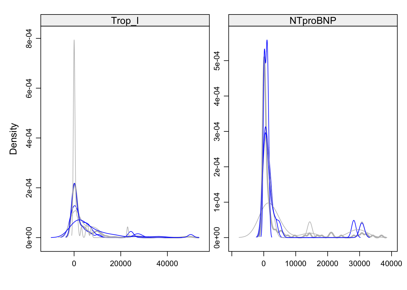
| Version | Author | Date |
|---|---|---|
| 3cbb66f | anjo1995 | 2026-03-06 |
# Create a data set with the observed and completed data
  table_clindat_imp <- complete(imputed_data, 1)

# Merge all data tables
  table_all_data <- table_lum_myo_healthy %>%
                    left_join(table_clindat_imp, by = "Study_ID")
Luminex Heatmap (Healthy, Cohort 1, Cohort 2)
# Prepare data table
  table_lum_myo_healthy <- table_lum_myo_healthy %>%
                           mutate(Cohort = case_when(Cohort == "Immpath" ~ "Cohort1",
                                           Cohort == "TUB_Myocarditis" ~ "Cohort2",
                                           TRUE ~ as.character(Cohort)))

# Name Rownames with study ID and remove Study ID and Cohort column
  rownames(table_lum_myo_healthy) <- table_lum_myo_healthy$Study_ID
  table_lum_myo_healthy_01 <- subset(table_lum_myo_healthy, select = -c(Study_ID, Cohort))

# Remove parameters if they are all the same in all groups
  table_lum_myo_healthy_01 <- Filter(var, table_lum_myo_healthy_01)

# Transpose Data Table
  table_lum_myo_healthy_01_t <- t(table_lum_myo_healthy_01)

##  Column Annotations
  # Create list with Study_ID & Cohort
    list_cohort_group <- subset(table_lum_myo_healthy, select= c(Study_ID, Cohort))
    rownames(list_cohort_group) <- list_cohort_group$Study_ID
    list_cohort_group <- subset(list_cohort_group, select= -c(Study_ID))

##  Row Annotations
  # Create list with Parameters
    list_parameter_groups <- read_xlsx("/Users/annajoachimbauer/Documents/Projects/ImmpathCarditis/Data Analysis/Data/Luminex/Grouping of Lumminex Marker.xlsx", sheet = "Groups")

# Create list with Columns of data table
  list_parameter_datatable <- as.data.frame(rownames(table_lum_myo_healthy_01_t))
  colnames(list_parameter_datatable) <- "Parameter"

# Merge to match the order of parameters
  list_parameter_groups_01 <- merge(list_parameter_groups, list_parameter_datatable, by.y = "Parameter")

# Define the predefined order for Group
  group_order <- c("Cytokines", "Chemokines", "Tissue Cytokines")

# Order list based on predefined order
  list_parameter_groups_02 <- list_parameter_groups_01 %>%
                              mutate(Group = factor(Group, levels = group_order)) %>%
                              arrange(Group)

  list_parameter_groups_03 <- unlist(list_parameter_groups_02$Parameter)

# Reorder Data Table based on the new ordered list
  table_lum_myo_healthy_01_t_ordered <- as.data.frame(table_lum_myo_healthy_01_t)
  table_lum_myo_healthy_01_t_ordered <- table_lum_myo_healthy_01_t_ordered[list_parameter_groups_03, , drop = FALSE]

# Convert it back to matrix
  table_lum_myo_healthy_01_t_ordered <- as.matrix(table_lum_myo_healthy_01_t_ordered)

# Log Transform
  table_lum_myo_healthy_01_t_ordered <- log2(table_lum_myo_healthy_01_t_ordered)

# Scale
  table_lum_myo_healthy_01_t_ordered <- t(apply(table_lum_myo_healthy_01_t_ordered, 1, scale))

# Create Cohort Label Colors of Annotations in heatmap
  ann_colors <- list(Cohort = c("Cohort2" = "orange", "Cohort1" = "royalblue4", "Healthy" = "grey"),
                   Group = c("Cytokines" = "darkseagreen", "Chemokines" = "lightblue", "Tissue Cytokines" = "mediumpurple3"))

## Column Annotation
    col_anno <- HeatmapAnnotation(df = list_cohort_group, col = ann_colors)

##  Row Annotation
  # Prepare row annotations as a data frame
    row_anno <- rowAnnotation(Group = list_parameter_groups_02$Group,
                              col = list(Group = c("Cytokines" = "darkseagreen",
                                                   "Chemokines" = "lightblue",
                                                   "Tissue Cytokines" = "mediumpurple3")))

# Create Heatmap
  heatmap_lum <- Heatmap(table_lum_myo_healthy_01_t_ordered,
                         name = "Expression",
                         col = circlize::colorRamp2(c(-5, 0, 5), c("blue", "white", "red")),
                         cluster_rows = FALSE,
                         cluster_columns = TRUE,
                         clustering_method_columns = "ward.D",
                         show_column_names = TRUE,
                         column_names_gp = gpar(fontsize = 8),
                         row_names_gp = gpar(fontsize = 8),
                         width = unit(10, "cm"), height = unit(17, "cm"),
                         right_annotation = row_anno,
                         top_annotation = col_anno)

# Draw Heatmap
  heatmap_lum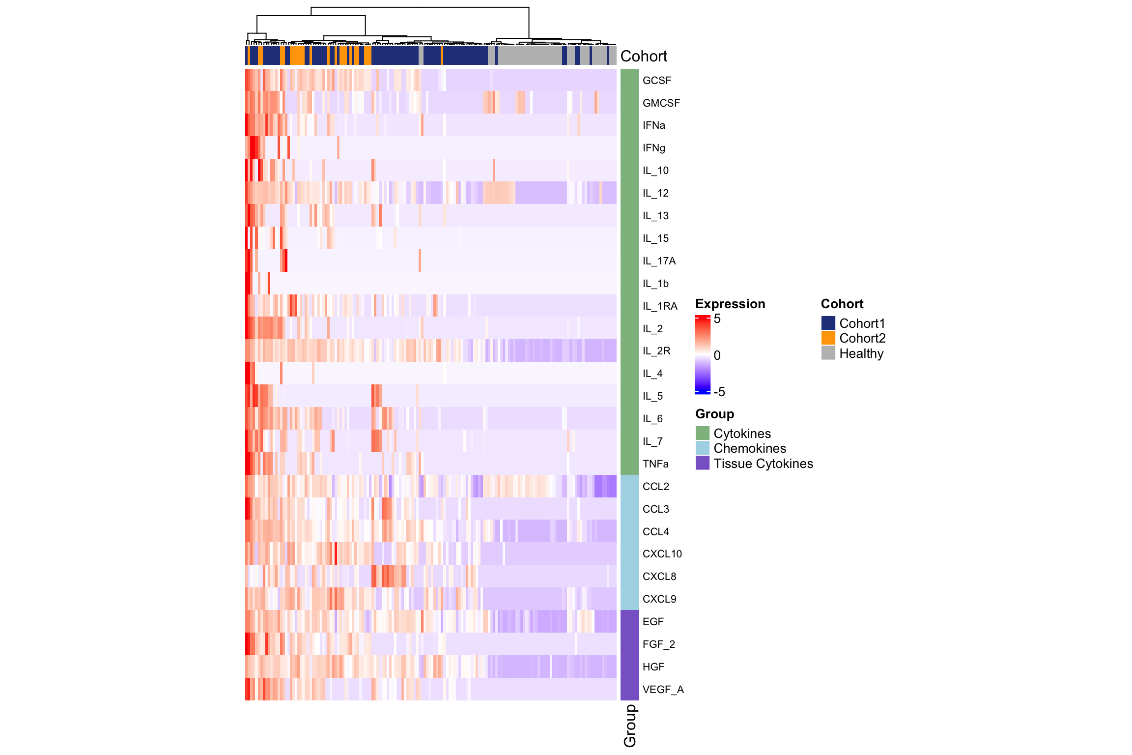
| Version | Author | Date |
|---|---|---|
| 3cbb66f | anjo1995 | 2026-03-06 |
Data Preparation (Cohort 1 & Healthy)
# Combine Tables
  table_lum_cohort1_healthy <- rbind(table_lum_cohort1, table_lum_healthy)

# Remove Columns with same value in all individuals (Variance  = 0)
  table_lum_cohort1_healthy <-  table_lum_cohort1_healthy %>%
                                select_if(~ !(is.numeric(.) && var(., na.rm = TRUE) == 0)) %>%
                                mutate(Cohort = case_when(Cohort == "Immpath" ~ "Cohort1",
                                       TRUE ~ as.character(Cohort)))
Volcano Plot (Cohort 1 & Healthy)
#  Set rownames
   rownames(table_lum_cohort1_healthy) <- table_lum_cohort1_healthy$Study_ID

# Calculate p-values between AM and healthy

  # Create the loop.vector (all the parameter columns)
    names(which(sapply(table_lum_cohort1_healthy, is.numeric) == TRUE)) -> parameters

  # Create table for stats
    table_lum_cohort1_healthy_stat <- data.table (Parameter = numeric(), group1 = character(),
                                              group2 = character(), n1 = numeric(),
                                              n2 = numeric(), statistic = numeric (),
                                              p = numeric (), p.signif = character(), FDR = numeric())

  # Create loop for calculation of stat test by parameter between cohort1 and healthy cohort
    for (i in parameters)

    {
      # Formula to insert parameter in loop
        formula = as.formula( paste(i, "Cohort", sep="~") )

        stat_parameter <- table_lum_cohort1_healthy %>%
                          wilcox_test(formula = formula) %>%
                          add_significance() %>%
                          mutate(FDR = p.adjust(p, method = "BH")) %>%
                          rename(Parameter = .y.)

      # Combine currently calculated stats with previous calculations
        table_lum_cohort1_healthy_stat <- rbind(table_lum_cohort1_healthy_stat, stat_parameter)
    }

# Calculate FC between AM and healthy

      # Calculate Mean of parameters per group
        table_lum_cohort1_healthy_log2  <- table_lum_cohort1_healthy %>%
                                           group_by(Cohort) %>%
                                           summarise(across(FGF_2:CXCL8, ~ mean(.x, na.rm = TRUE)))

      # Transverse Data Table and set rownames
        table_lum_cohort1_healthy_log2_t  <- table_lum_cohort1_healthy_log2  %>%
                                             t %>%
                                             as.data.frame() %>%
                                             row_to_names(1)

     # Convert whole data table to numeric
       table_lum_cohort1_healthy_log2_t  <- mutate_all(table_lum_cohort1_healthy_log2_t,
                                                   function(x) as.numeric(as.character(x)))

     # Calculate FC between healthy and cohort1
       table_lum_cohort1_healthy_log2_t$log2_fc <- log2(table_lum_cohort1_healthy_log2_t$Cohort1 /
                                                        table_lum_cohort1_healthy_log2_t$Healthy)

     # Add p-values to data table
        # Extract only Parameters and p-values
           stat.test_p <- table_lum_cohort1_healthy_stat %>%
                          dplyr::select(Parameter, FDR)

        # Merge data tables (log2, FC, p val)
          table_lum_cohort1_healthy_log2_t$Parameter <- rownames(table_lum_cohort1_healthy_log2_t)
          table_lum_cohort1_healthy_volcano <- merge(table_lum_cohort1_healthy_log2_t, stat.test_p, by = "Parameter")

  # Create Volcano Plot

       # Mark parameters if FC > 1.5 = upregulated
         table_lum_cohort1_healthy_volcano$diff_expression <- ifelse (table_lum_cohort1_healthy_volcano$log2_fc > 1.5,
                                                                      "up", "no")

       # Add new column to relabel parameters FC of > 1.5
         table_lum_cohort1_healthy_volcano$label_para <- ifelse (table_lum_cohort1_healthy_volcano$log2_fc > 1.5,
                                                                table_lum_cohort1_healthy_volcano$Parameter, "")

   plot_volcano <- EnhancedVolcano(table_lum_cohort1_healthy_volcano,
                                   lab = table_lum_cohort1_healthy_volcano$label_para,
                                   x = 'log2_fc', y = 'FDR',
                                   FCcutoff = 1.5, pointSize = 3.5, labSize = 4, colAlpha = 0.7,
                                   boxedLabels = TRUE, col = c("grey", "grey", "grey", "royalblue4"),
                                   xlab = bquote(~Log[2]~ "fold change"), ylab = bquote("FDR-adjusted p-value"),
                                   xlim = c(0, 4), ylim = c(0, 21), pCutoff = 0.05,
                                   title = NULL, subtitle = NULL, border = 'full',
                                   drawConnectors = TRUE,widthConnectors = 0.5, colConnectors = "royalblue4") +
                                   theme_classic() +
                                   theme(panel.grid = element_blank(),
                                         panel.border = element_rect(colour = "black", fill = NA,),
                                         legend.position = "none")

   print( plot_volcano)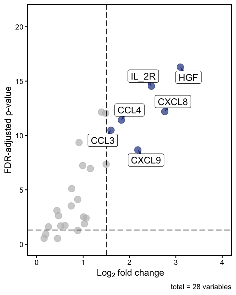
| Version | Author | Date |
|---|---|---|
| 3cbb66f | anjo1995 | 2026-03-06 |
Data Preparation (Cohort 2 & Healthy)
# Combine Tables
  table_lum_cohort2_healthy <- rbind(table_lum_cohort2, table_lum_healthy)

# Remove Columns with same value in all individuals (Variance  = 0)
  table_lum_cohort2_healthy <- table_lum_cohort2_healthy %>%
                                select_if(~ !(is.numeric(.) && var(., na.rm = TRUE) == 0)) %>%
                                mutate(Cohort = case_when(Cohort == "TUB_Myocarditis" ~ "Cohort2",
                                       TRUE ~ as.character(Cohort)))
Volcano Plot (Cohort 2 & Healthy)
#  Set rownames
   rownames(table_lum_cohort2_healthy) <- table_lum_cohort2_healthy$Study_ID

# Calculate p-values between AM and healthy

  # Create the loop.vector (all the parameter columns)
    names(which(sapply(table_lum_cohort2_healthy, is.numeric) == TRUE)) -> parameters

  # Create table for stats
    table_lum_cohort2_healthy_stat <- data.table (Parameter = numeric(), group1 = character(),
                                              group2 = character(), n1 = numeric(),
                                              n2 = numeric(), statistic = numeric (),
                                              p = numeric (), p.signif = character(), FDR = numeric())

  # Create loop for calculation of stat test by parameter between cohort1 and healthy cohort
    for (i in parameters)

    {
      # Formula to insert parameter in loop
        formula = as.formula( paste(i, "Cohort", sep="~") )

        stat_parameter <- table_lum_cohort2_healthy %>%
                          wilcox_test(formula = formula) %>%
                          add_significance() %>%
                          mutate(FDR = p.adjust(p, method = "BH")) %>%
                          rename(Parameter = .y.)

      # Combine currently calculated stats with previous calculations
        table_lum_cohort2_healthy_stat <- rbind(table_lum_cohort2_healthy_stat, stat_parameter)
    }

# Calculate FC between AM and healthy

      # Calculate Mean of parameters per group
        table_lum_cohort2_healthy_log2  <- table_lum_cohort2_healthy %>%
                                           group_by(Cohort) %>%
                                           summarise(across(FGF_2:CXCL8, ~ mean(.x, na.rm = TRUE)))

      # Transverse Data Table and set rownames
        table_lum_cohort2_healthy_log2_t  <- table_lum_cohort2_healthy_log2  %>%
                                             t %>%
                                             as.data.frame() %>%
                                             row_to_names(1)

     # Convert whole data table to numeric
       table_lum_cohort2_healthy_log2_t  <- mutate_all(table_lum_cohort2_healthy_log2_t,
                                                   function(x) as.numeric(as.character(x)))

     # Calculate FC between healthy and cohort1
       table_lum_cohort2_healthy_log2_t$log2_fc <- log2(table_lum_cohort2_healthy_log2_t$Cohort2 /
                                                        table_lum_cohort2_healthy_log2_t$Healthy)

     # Add p-values to data table
        # Extract only Parameters and p-values
           stat.test_p <- table_lum_cohort2_healthy_stat %>%
                          dplyr::select(Parameter, FDR)

        # Merge data tables (log2, FC, p val)
          table_lum_cohort2_healthy_log2_t$Parameter <- rownames(table_lum_cohort2_healthy_log2_t)
          table_lum_cohort2_healthy_volcano <- merge(table_lum_cohort2_healthy_log2_t, stat.test_p, by = "Parameter")

  # Create Volcano Plot

       # Mark parameters if FC > 1.5 = upregulated
         table_lum_cohort2_healthy_volcano$diff_expression <- ifelse (table_lum_cohort2_healthy_volcano$log2_fc > 1.5,
                                                                      "up", "no")

       # Add new column to relabel parameters FC of > 1.5
         table_lum_cohort2_healthy_volcano$label_para <- ifelse (table_lum_cohort2_healthy_volcano$log2_fc > 1.5,
                                                                 table_lum_cohort2_healthy_volcano$Parameter, "")

   plot_volcano <- EnhancedVolcano(table_lum_cohort2_healthy_volcano,
                                   lab = table_lum_cohort2_healthy_volcano$label_para,
                                   x = 'log2_fc', y = 'FDR',
                                   FCcutoff = 1.5, pointSize = 3.5, labSize = 4, colAlpha = 0.7,
                                   boxedLabels = TRUE, col = c("grey", "grey", "grey", "orange"),
                                   xlab = bquote(~Log[2]~ "fold change"), ylab = bquote("FDR-adjusted p-value"),
                                   xlim = c(0, 4), ylim = c(0, 21), pCutoff = 0.05,
                                   title = NULL, subtitle = NULL, border = 'full',
                                   drawConnectors = TRUE,widthConnectors = 0.5, colConnectors = "orange") +
                                   theme_classic() +
                                   theme(panel.grid = element_blank(),
                                         panel.border = element_rect(colour = "black", fill = NA,),
                                         legend.position = "none")

   print( plot_volcano)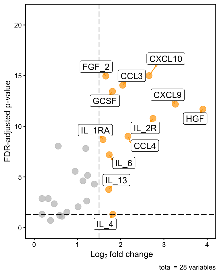
| Version | Author | Date |
|---|---|---|
| 3cbb66f | anjo1995 | 2026-03-06 |
Comparison AM Cohort & Healthy selected parameters
# Subset Data Table
  rownames(table_lum_myo_healthy) <- table_lum_myo_healthy$Study_ID

  table_lum_myo_healthy_01 <- table_lum_myo_healthy

# Rename Cohorts to combine myocarditis patients
  table_lum_myo_healthy_01$Cohort <- ifelse(table_lum_myo_healthy_01$Cohort == "Healthy", "Healthy", "Myocarditis")


  # Prepare data table
     table_para <- table_lum_myo_healthy_01 %>%
                   pivot_longer(cols = where(is.numeric),
                                names_to = "Parameter",
                                values_to = "Parameter_val")

  # Log Transform Parameters
    table_para$Parameter_val_log10 <- log10(table_para$Parameter_val)

# Calculate Stats
  # Wilcox Test
    stat.test <- table_para %>%
                 group_by(Parameter) %>%
                 wilcox_test(Parameter_val ~ Cohort) %>%
                 add_significance()  %>%
                 mutate(p_adj = p.adjust(p, method = "BH"))

    # Get max value per parameter (for p-value position)
      max_y <- table_para %>%
               group_by(Parameter) %>%
               summarise(max_val = max(Parameter_val, na.rm = TRUE))

    # Get min value per parameter (for y limits)
      min_y <- table_para %>%
               group_by(Parameter) %>%
               summarise(min_val = min(Parameter_val, na.rm = TRUE))

    # Combine with max_y info for plotting
      stat.test <-  stat.test %>%
                    left_join(max_y, by = "Parameter") %>%
                    mutate(y.position = max_val * 1)

# Create the loop to create a plot
    param <- c("HGF", "IL_2R", "CCL3", "CCL4")

  # Create a list for all plots created in the loop
    plots_list <- list()
    for (param in param)

      {
        # Filter for the data
          temp_data <- table_para %>%
                       filter(Parameter == param)

          temp_stat_test <- stat.test %>%
                            filter(Parameter == param) %>%
                            mutate(p_adj_label = ifelse(p_adj < 0.001, "<0.001", sprintf("%.3f", p_adj)))

          temp_stat_test <- temp_stat_test %>%
                            mutate(y.position = 30000 / 1.2)

        # Plot Boxplot
          plot <-  ggplot(temp_data, aes(x = Cohort, y = Parameter_val)) +
                   geom_boxplot(aes(fill = Cohort), color = "black", outlier.shape = NA,
                                     width = 0.6, alpha = 0.4) +
                   geom_point(shape = 21, size = 3, color = "black", aes(fill = Cohort),
                              position = position_jitter(width = 0.2, height = 0)) +
                   scale_y_log10(labels = function(x) format(x, scientific = FALSE, trim = TRUE),
                                 limits = c(NA, 30000),
                                 expand = expansion(mult = c(0.05, 0), add = c(0,0))) +
                   scale_fill_manual(values = c("Myocarditis" = "darkred",
                                                "Healthy" = "grey")) +
                   stat_pvalue_manual(temp_stat_test,label = "p_adj_label",
                                      y.position = log10(temp_stat_test$y.position),
                                      tip.length = 0) +
                   labs(x = NULL, y = paste0(param, " (pg/ml)")) +
                   theme_classic() +
                   theme(axis.title.x = element_blank(),
                         axis.text.x  = element_blank(),
                         axis.ticks.x = element_blank(),
                         legend.position = "none")

          plots_list[[param]] <- plot
      }

# Create the loop to create a plot
    param <- c("CXCL9", "CXCL10", "IL_6", "CXCL8")

  # Create a list for all plots created in the loop
    plots_list_2 <- list()
    for (param in param)

      {
        # Filter for the data
          temp_data <- table_para %>%
                       filter(Parameter == param)

          temp_stat_test <- stat.test %>%
                            filter(Parameter == param) %>%
                            mutate(p_adj_label = ifelse(p_adj < 0.001, "<0.001", sprintf("%.3f", p_adj)))

          temp_stat_test <- temp_stat_test %>%
                            mutate(y.position = 10000 / 1.2)

        # Plot Boxplot
          plot <-  ggplot(temp_data, aes(x = Cohort, y = Parameter_val)) +
                   geom_boxplot(aes(fill = Cohort), color = "black", outlier.shape = NA,
                                     width = 0.6, alpha = 0.4) +
                   geom_point(shape = 21, size = 3, color = "black", aes(fill = Cohort),
                              position = position_jitter(width = 0.2, height = 0)) +
                   scale_y_log10(labels = function(x) format(x, scientific = FALSE, trim = TRUE),
                                 limits = c(NA, 10000), breaks = c(100, 300, 1000, 3000, 10000),
                                 expand = expansion(mult = c(0.05, 0), add = c(0,0))) +
                   scale_fill_manual(values = c("Myocarditis" = "darkred",
                                                "Healthy" = "grey")) +
                   stat_pvalue_manual(temp_stat_test,label = "p_adj_label",
                                      y.position = log10(temp_stat_test$y.position),
                                      tip.length = 0) +
                   labs(x = NULL, y = paste0(param, " (pg/ml)")) +
                   theme_classic() +
                   theme(axis.title.x = element_blank(),
                         axis.text.x  = element_blank(),
                         axis.ticks.x = element_blank(),
                         legend.position = "none")

          plots_list_2[[param]] <- plot
      }

   # Combine plots to a panel
      panel <-  ggarrange(plotlist = c(plots_list, plots_list_2),
                ncol = 4, nrow = ceiling(length(plots_list) / 3),
                common.legend = TRUE)

      print(panel)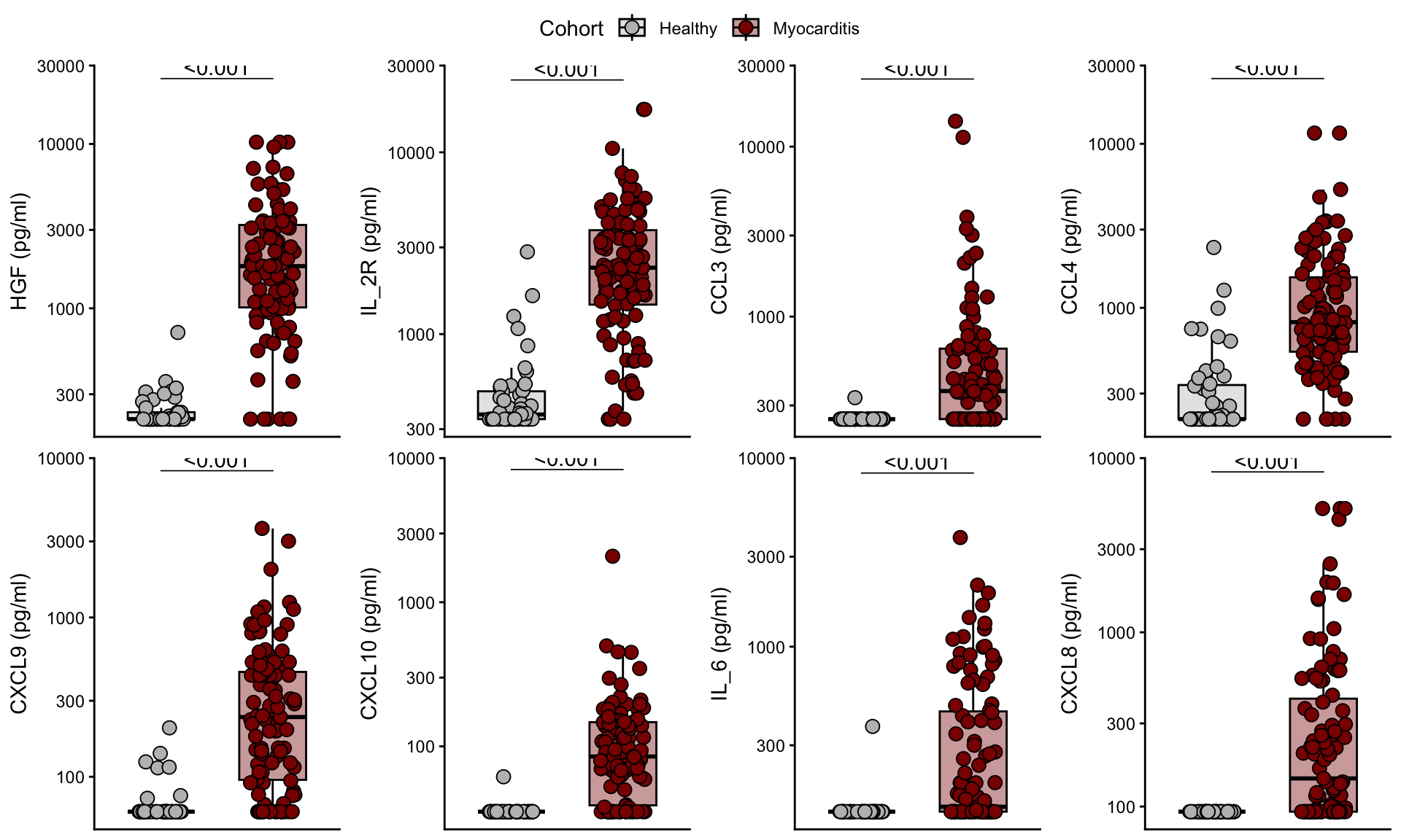
| Version | Author | Date |
|---|---|---|
| 3cbb66f | anjo1995 | 2026-03-06 |
Correlation Plots NTproBNP & selected Parameters (Healthy, Cohort 1, Cohort 2)
# Rename Cohorts
  table_corr <- table_all_data %>%
                mutate(Cohort = if_else (Cohort == "Healthy", "Healthy", "Myocarditis"))

# Fixed variable
  fixed_param <- "NTproBNP"

# Create the loop to create a plot
  biomarkers <- c("CXCL9","CCL4", "CCL3", "CXCL8", "IL_6")
  x_settings <- list(CXCL9 = list(limits = c(NA, 10000),  breaks = c(300, 1000, 3000, 10000)),
                     CCL4 = list(limits = c(NA, 30000), breaks = c(100, 300, 1000, 3000, 10000, 30000)),
                     CCL3 = list(limits = c(NA, 30000), breaks = c(100, 300, 1000, 3000, 10000, 30000)),
                     CXCL8 = list(limits = c(NA, 10000), breaks = c(100, 300, 1000, 3000, 10000)),
                     IL_6 = list(limits = c(NA, 10000), breaks = c(100, 300, 1000, 3000, 10000)))

# Define axis labels for each biomarker
  biomarker_labels <- c("CXCL9 (pg/ml)", "CCL4 (pg/ml)", "CCL3 (pg/ml)", "CXCL8 (pg/ml)", "IL-6 (pg/ml)")
  names(biomarker_labels) <- biomarkers

# Create list for plots
  plots_list <- list()

# Loop Correlation Plot
  for (p in biomarkers)

    {

      # Compute Spearman correlation
        cor_test <- cor.test(table_corr$NTproBNP, table_corr[[p]], method = "spearman")

      # Axis settings
        x_lim <- x_settings[[p]]$limits
        x_brk <- x_settings[[p]]$breaks

      # Scatter plot with regression line
        plot <- ggplot(table_corr, aes(x = .data[[p]], y = NTproBNP)) +
                geom_point(shape = 21, size = 3, color = "black", aes(fill = Cohort),
                             position = position_jitter(width = 0.05, height = 0)) +
                geom_smooth(method = "lm", se = TRUE, color = "black") +
                scale_fill_manual(values = c("Myocarditis" = "darkred",
                                                     "Healthy" = "grey")) +
                scale_x_log10(labels = function(x) format(x, scientific = FALSE, trim = TRUE),
                                      limits = x_lim, breaks = x_brk, expand = expansion(mult = c(0.05, 0))) +
                scale_y_log10(labels = function(x) format(x, scientific = FALSE, trim = TRUE),
                              limits = c(10, 100000), expand = c(0, 0)) +
                theme_classic() +
                labs(x = biomarker_labels[[p]], y = "NT-proBNP (ng/l)") +
                annotate("text", x = min(table_corr[[p]], na.rm = TRUE),
                                 y = min(table_corr$LV_EF, na.rm = TRUE),
                                label = paste0("r = ", round(cor_test$estimate, 2),
                                        "\np = ", ifelse(cor_test$p.value < 0.001, "< 0.001",signif(cor_test$p.value, 3))),
                         hjust = 0, vjust = 1, size = 4)

      # Store each plot
      plots_list[[p]] <- plot

  }

# Combine plots to a panel
  panel <-  ggarrange(plotlist = plots_list,
                      ncol = 3,
                      nrow = ceiling(length(plots_list) / 2),
                      common.legend = TRUE)

  print(panel)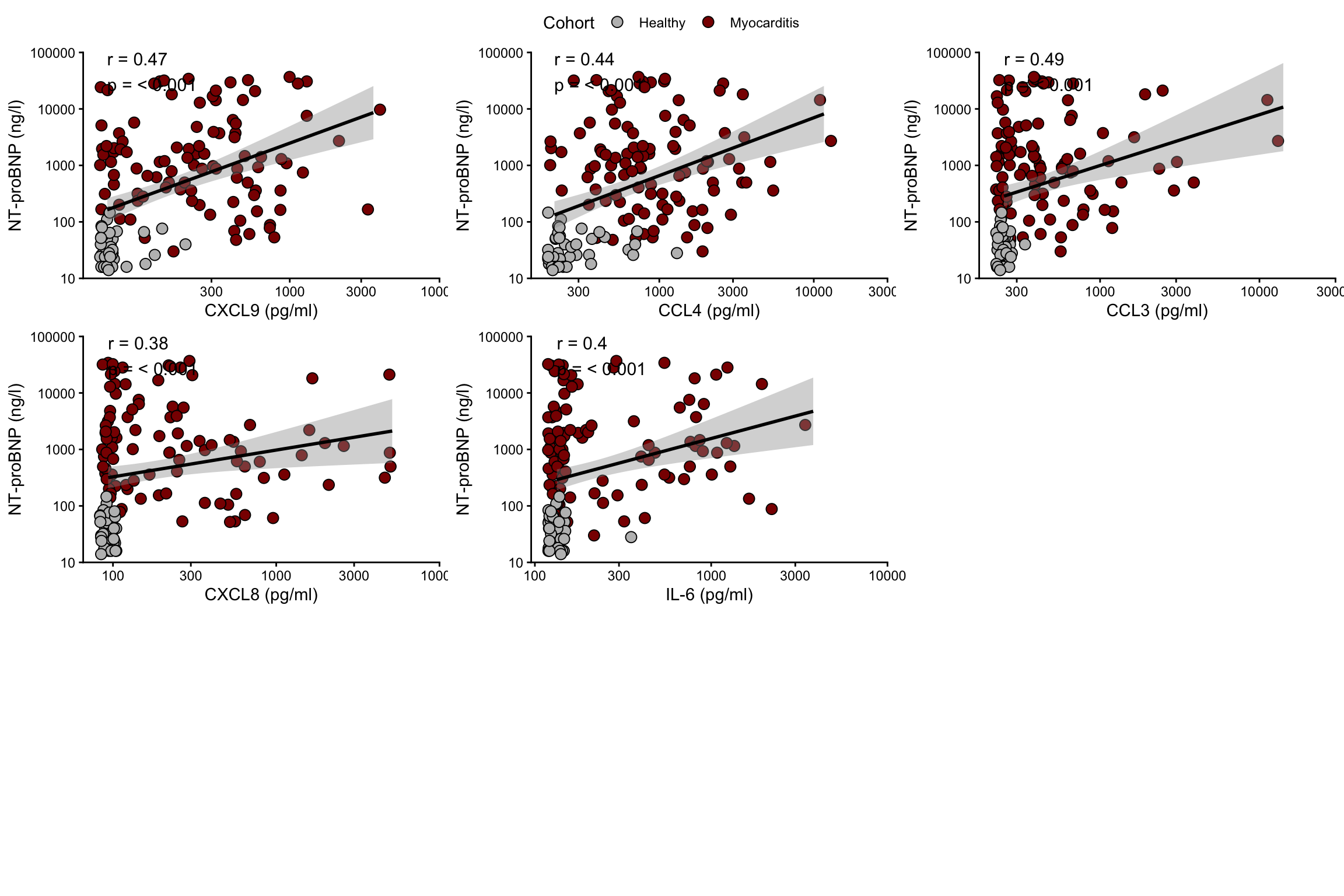
| Version | Author | Date |
|---|---|---|
| 3cbb66f | anjo1995 | 2026-03-06 |
Comparison AM Cohorts & Healthy fibroblast-derived factors
# Subset Data Table
  table_lum_myo_healthy_01 <- table_lum_myo_healthy %>%
                              dplyr::select(EGF, FGF_2, VEGF_A, Cohort)

# Rename Cohorts to combine myocarditis patients
  table_lum_myo_healthy_01$Cohort <- ifelse(table_lum_myo_healthy_01$Cohort == "Healthy", "Healthy", "Myocarditis")


# Prepare data table
  table_para <- table_lum_myo_healthy_01 %>%
                pivot_longer(cols = where(is.numeric),
                             names_to = "Parameter",
                             values_to = "Parameter_val")

# Log Transform Parameters
  table_para$Parameter_val_log10 <- log10(table_para$Parameter_val)

# Calculate Stats
    # Wilcox Test
      stat.test <- table_para %>%
                   group_by(Parameter) %>%
                   wilcox_test(Parameter_val ~ Cohort) %>%
                   add_significance()  %>%
                   mutate(p_adj = p.adjust(p, method = "BH"))

    # Get max value per parameter (for p-value position)
      max_y <- table_para %>%
               group_by(Parameter) %>%
               summarise(max_val = max(Parameter_val, na.rm = TRUE))

    # Get min value per parameter (for y limits)
      min_y <- table_para %>%
               group_by(Parameter) %>%
               summarise(min_val = min(Parameter_val, na.rm = TRUE))

    # Combine with max_y info for plotting
      stat.test <-  stat.test %>%
                    left_join(max_y, by = "Parameter") %>%
                    mutate(y.position = max_val * 1)

# Define Parameters and axis settings
  param <- c("EGF", "FGF_2", "VEGF_A")

  y_settings <- list(EGF = list(limits = c(NA, 10000), breaks = c(100, 300, 1000, 3000, 10000)),
                     FGF_2  = list(limits = c(NA, 3000),  breaks = c(100, 300, 1000, 3000)),
                     VEGF_A = list(limits = c(NA, 1000),  breaks = c(100, 300, 1000)))

# Define axis labels for each biomarker
  biomarker_labels <- c("EGF (pg/ml)", "FGF-2 (pg/ml)", "VEGF-A (pg/ml)")
  names(biomarker_labels) <- param

# Create a list for all plots created in the loop
  plots_list <- list()
  for (param in param)

  {
      # Axis settings
        y_lim <- y_settings[[param]]$limits
        y_brk <- y_settings[[param]]$breaks

      # Filter for the data
        temp_data <- table_para %>%
                     filter(Parameter == param)

        temp_stat_test <- stat.test %>%
                          filter(Parameter == param) %>%
                          mutate(p_adj_label = ifelse(p_adj < 0.001, "<0.001", sprintf("%.3f", p_adj)))

        temp_stat_test <- temp_stat_test %>%
                          mutate(y.position = max(y_lim, na.rm = TRUE) / 1.2)

      # Plot Boxplot
        plot <-  ggplot(temp_data, aes(x = Cohort, y = Parameter_val)) +
                 geom_boxplot(aes(fill = Cohort), color = "black", outlier.shape = NA,
                                     width = 0.6, alpha = 0.4) +
                 geom_point(shape = 21, size = 3, color = "black", aes(fill = Cohort),
                              position = position_jitter(width = 0.2, height = 0)) +
                 scale_y_log10(labels = function(x) format(x, scientific = FALSE, trim = TRUE),
                                  limits = y_lim, breaks = y_brk, expand = expansion(mult = c(0.05, 0))) +
                 scale_fill_manual(values = c("Myocarditis" = "darkred",
                                                "Healthy" = "grey")) +
                 stat_pvalue_manual(temp_stat_test,label = "p_adj_label",
                                      y.position = log10(temp_stat_test$y.position),
                                      tip.length = 0) +
                 labs(x = NULL, y = biomarker_labels[[param]]) +
                 theme_classic() +
                 theme(axis.title.x = element_blank(),
                       axis.text.x  = element_blank(),
                       axis.ticks.x = element_blank(),
                       legend.position = "none")

        plots_list[[param]] <- plot
    }

   # Combine plots to a panel
     panel <-  ggarrange(plotlist = plots_list,
               ncol = 3, nrow = 1,
               common.legend = TRUE)

     print(panel)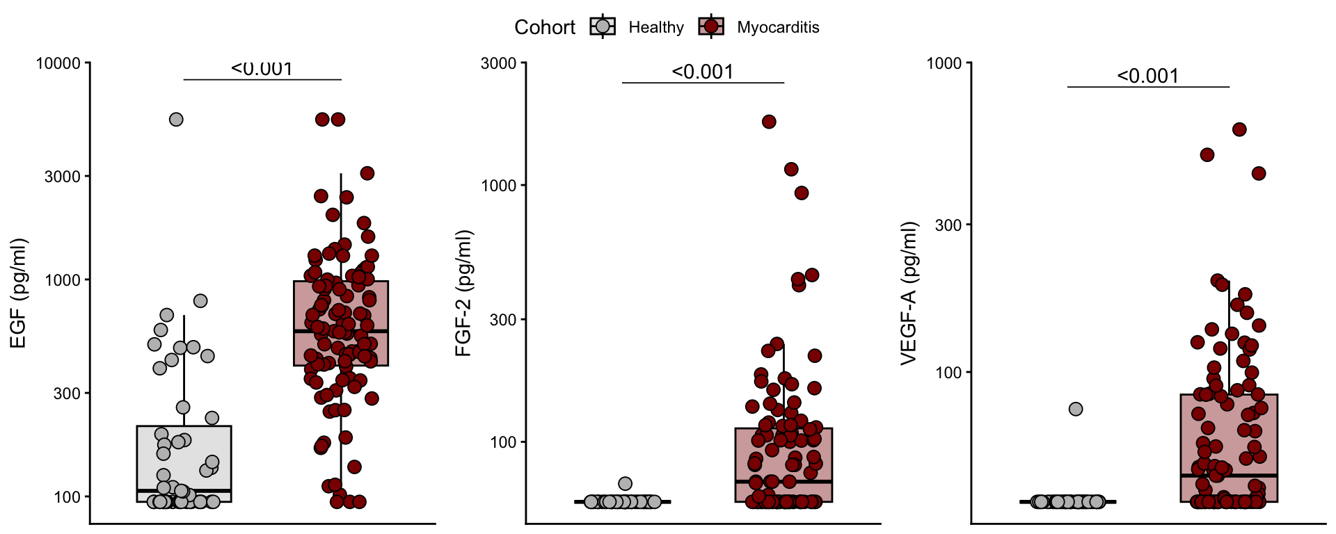
| Version | Author | Date |
|---|---|---|
| 3cbb66f | anjo1995 | 2026-03-06 |
session info
sessionInfo()R version 4.4.3 (2025-02-28)
Platform: aarch64-apple-darwin20
Running under: macOS 26.3
Matrix products: default
BLAS: /Library/Frameworks/R.framework/Versions/4.4-arm64/Resources/lib/libRblas.0.dylib
LAPACK: /Library/Frameworks/R.framework/Versions/4.4-arm64/Resources/lib/libRlapack.dylib; LAPACK version 3.12.0
locale:
[1] en_US.UTF-8/en_US.UTF-8/en_US.UTF-8/C/en_US.UTF-8/en_US.UTF-8
time zone: Europe/Zurich
tzcode source: internal
attached base packages:
[1] grid stats graphics grDevices utils datasets methods
[8] base
other attached packages:
[1] ImmunoLogic_0.0.0.9000 Seurat_5.3.1 SeuratObject_5.2.0
[4] sp_2.2-0 kernlab_0.9-33 dbscan_1.2-0
[7] umap_0.2.10.0 Rtsne_0.17 cluster_2.1.8
[10] factoextra_1.0.7 randomForest_4.7-1.2 pROC_1.19.0.1
[13] mice_3.18.0 caret_7.0-1 lattice_0.22-6
[16] drc_3.0-1 logistf_1.26.1 glmnet_4.1-10
[19] Matrix_1.7-2 broom_1.0.11 MuMIn_1.48.11
[22] Hmisc_5.2-3 car_3.1-3 carData_3.0-5
[25] multcomp_1.4-28 TH.data_1.1-4 MASS_7.3-65
[28] survival_3.8-3 mvtnorm_1.3-3 rstatix_0.7.3
[31] ggpattern_1.2.1 gridExtra_2.3 cowplot_1.2.0
[34] patchwork_1.3.2 plotly_4.11.0 EnhancedVolcano_1.24.0
[37] RColorBrewer_1.1-3 circlize_0.4.16 ComplexHeatmap_2.22.0
[40] pheatmap_1.0.12 corrplot_0.95 ggcorrplot_0.1.4.1
[43] ggbeeswarm_0.7.2 ggrepel_0.9.6 ggpubr_0.6.2
[46] readxl_1.4.5 writexl_1.5.0 openxlsx_4.2.5.2
[49] gtsummary_2.4.0 flextable_0.9.6 tableone_0.13.2
[52] table1_1.4.3 scales_1.4.0 here_1.0.2
[55] janitor_2.2.0 magrittr_2.0.4 data.table_1.17.8
[58] lubridate_1.9.4 forcats_1.0.1 stringr_1.6.0
[61] dplyr_1.1.4 purrr_1.2.0 readr_2.1.6
[64] tidyr_1.3.1 tibble_3.3.0 ggplot2_4.0.1
[67] tidyverse_2.0.0
loaded via a namespace (and not attached):
[1] IRanges_2.40.1 nnet_7.3-20 goftest_1.2-3
[4] vctrs_0.6.5 spatstat.random_3.4-3 digest_0.6.39
[7] png_0.1-8 shape_1.4.6.1 git2r_0.36.2
[10] alabama_2023.1.0 deldir_2.0-4 httpcode_0.3.0
[13] parallelly_1.45.1 fontLiberation_0.1.0 reshape2_1.4.5
[16] httpuv_1.6.16 foreach_1.5.2 BiocGenerics_0.52.0
[19] withr_3.0.2 xfun_0.54 crul_1.4.2
[22] emmeans_1.10.4 systemfonts_1.3.1 ragg_1.5.0
[25] zoo_1.8-14 GlobalOptions_0.1.3 gtools_3.9.5
[28] pbapply_1.7-4 Formula_1.2-5 promises_1.5.0
[31] otel_0.2.0 httr_1.4.7 globals_0.18.0
[34] fitdistrplus_1.2-4 rstudioapi_0.17.1 pan_1.9
[37] miniUI_0.1.2 generics_0.1.4 base64enc_0.1-3
[40] curl_7.0.0 S4Vectors_0.44.0 mitools_2.4
[43] polyclip_1.10-7 quadprog_1.5-8 xtable_1.8-4
[46] doParallel_1.0.17 evaluate_1.0.5 hms_1.1.4
[49] irlba_2.3.5.1 colorspace_2.1-2 polynom_1.4-1
[52] ROCR_1.0-11 reticulate_1.44.1 spatstat.data_3.1-9
[55] lmtest_0.9-40 snakecase_0.11.1 later_1.4.4
[58] spatstat.geom_3.6-1 future.apply_1.20.0 scattermore_1.2
[61] survey_4.4-2 matrixStats_1.5.0 RcppAnnoy_0.0.22
[64] class_7.3-23 pillar_1.11.1 nlme_3.1-167
[67] iterators_1.0.14 compiler_4.4.3 RSpectra_0.16-2
[70] stringi_1.8.7 gower_1.0.2 jomo_2.7-6
[73] tensor_1.5.1 minqa_1.2.8 plyr_1.8.9
[76] crayon_1.5.3 abind_1.4-8 orthopolynom_1.0-6.1
[79] sandwich_3.1-1 whisker_0.4.1 codetools_0.2-20
[82] textshaping_1.0.4 basefun_1.2-4 recipes_1.3.1
[85] openssl_2.3.4 bslib_0.9.0 GetoptLong_1.0.5
[88] mime_0.13 splines_4.4.3 Rcpp_1.1.0
[91] fastDummies_1.7.5 coneproj_1.20 variables_1.1-2
[94] cellranger_1.1.0 knitr_1.50 clue_0.3-66
[97] lme4_1.1-38 fs_1.6.6 listenv_0.10.0
[100] checkmate_2.3.3 Rdpack_2.6.4 ggsignif_0.6.4
[103] estimability_1.5.1 tzdb_0.5.0 pkgconfig_2.0.3
[106] tools_4.4.3 cachem_1.1.0 rbibutils_2.4
[109] numDeriv_2016.8-1.1 viridisLite_0.4.2 DBI_1.2.3
[112] fastmap_1.2.0 rmarkdown_2.30 ica_1.0-3
[115] tram_1.2-4 sass_0.4.10 officer_0.6.6
[118] coda_0.19-4.1 dotCall64_1.2 RANN_2.6.2
[121] rpart_4.1.24 farver_2.1.2 reformulas_0.4.2
[124] mgcv_1.9-1 yaml_2.3.11 workflowr_1.7.2
[127] foreign_0.8-88 cli_3.6.5 stats4_4.4.3
[130] lifecycle_1.0.4 uwot_0.2.4 askpass_1.2.1
[133] lava_1.8.0 backports_1.5.0 mlt_1.6-6
[136] timechange_0.3.0 gtable_0.3.6 rjson_0.2.23
[139] ggridges_0.5.7 progressr_0.18.0 parallel_4.4.3
[142] jsonlite_2.0.0 RcppHNSW_0.6.0 mitml_0.4-5
[145] qrng_0.0-10 spatstat.utils_3.2-0 zip_2.3.1
[148] jquerylib_0.1.4 spatstat.univar_3.1-5 timeDate_4051.111
[151] lazyeval_0.2.2 shiny_1.12.0 htmltools_0.5.9
[154] sctransform_0.4.2 glue_1.8.0 gfonts_0.2.0
[157] BB_2019.10-1 spam_2.11-1 gdtools_0.3.7
[160] rprojroot_2.1.1 boot_1.3-31 igraph_2.2.1
[163] R6_2.6.1 labeling_0.4.3 ipred_0.9-15
[166] nloptr_2.2.1 tidyselect_1.2.1 vipor_0.4.7
[169] plotrix_3.8-4 htmlTable_2.4.3 operator.tools_1.6.3
[172] xml2_1.5.1 fontBitstreamVera_0.1.1 future_1.68.0
[175] ModelMetrics_1.2.2.2 KernSmooth_2.23-26 S7_0.2.1
[178] fontquiver_0.2.1 htmlwidgets_1.6.4 rlang_1.1.6
[181] spatstat.sparse_3.1-0 spatstat.explore_3.6-0 uuid_1.2-1
[184] formula.tools_1.7.1 hardhat_1.4.1 beeswarm_0.4.0
[187] prodlim_2023.08.28 date()[1] "Fri Mar 6 14:27:36 2026"
sessionInfo()R version 4.4.3 (2025-02-28)
Platform: aarch64-apple-darwin20
Running under: macOS 26.3
Matrix products: default
BLAS: /Library/Frameworks/R.framework/Versions/4.4-arm64/Resources/lib/libRblas.0.dylib
LAPACK: /Library/Frameworks/R.framework/Versions/4.4-arm64/Resources/lib/libRlapack.dylib; LAPACK version 3.12.0
locale:
[1] en_US.UTF-8/en_US.UTF-8/en_US.UTF-8/C/en_US.UTF-8/en_US.UTF-8
time zone: Europe/Zurich
tzcode source: internal
attached base packages:
[1] grid stats graphics grDevices utils datasets methods
[8] base
other attached packages:
[1] ImmunoLogic_0.0.0.9000 Seurat_5.3.1 SeuratObject_5.2.0
[4] sp_2.2-0 kernlab_0.9-33 dbscan_1.2-0
[7] umap_0.2.10.0 Rtsne_0.17 cluster_2.1.8
[10] factoextra_1.0.7 randomForest_4.7-1.2 pROC_1.19.0.1
[13] mice_3.18.0 caret_7.0-1 lattice_0.22-6
[16] drc_3.0-1 logistf_1.26.1 glmnet_4.1-10
[19] Matrix_1.7-2 broom_1.0.11 MuMIn_1.48.11
[22] Hmisc_5.2-3 car_3.1-3 carData_3.0-5
[25] multcomp_1.4-28 TH.data_1.1-4 MASS_7.3-65
[28] survival_3.8-3 mvtnorm_1.3-3 rstatix_0.7.3
[31] ggpattern_1.2.1 gridExtra_2.3 cowplot_1.2.0
[34] patchwork_1.3.2 plotly_4.11.0 EnhancedVolcano_1.24.0
[37] RColorBrewer_1.1-3 circlize_0.4.16 ComplexHeatmap_2.22.0
[40] pheatmap_1.0.12 corrplot_0.95 ggcorrplot_0.1.4.1
[43] ggbeeswarm_0.7.2 ggrepel_0.9.6 ggpubr_0.6.2
[46] readxl_1.4.5 writexl_1.5.0 openxlsx_4.2.5.2
[49] gtsummary_2.4.0 flextable_0.9.6 tableone_0.13.2
[52] table1_1.4.3 scales_1.4.0 here_1.0.2
[55] janitor_2.2.0 magrittr_2.0.4 data.table_1.17.8
[58] lubridate_1.9.4 forcats_1.0.1 stringr_1.6.0
[61] dplyr_1.1.4 purrr_1.2.0 readr_2.1.6
[64] tidyr_1.3.1 tibble_3.3.0 ggplot2_4.0.1
[67] tidyverse_2.0.0
loaded via a namespace (and not attached):
[1] IRanges_2.40.1 nnet_7.3-20 goftest_1.2-3
[4] vctrs_0.6.5 spatstat.random_3.4-3 digest_0.6.39
[7] png_0.1-8 shape_1.4.6.1 git2r_0.36.2
[10] alabama_2023.1.0 deldir_2.0-4 httpcode_0.3.0
[13] parallelly_1.45.1 fontLiberation_0.1.0 reshape2_1.4.5
[16] httpuv_1.6.16 foreach_1.5.2 BiocGenerics_0.52.0
[19] withr_3.0.2 xfun_0.54 crul_1.4.2
[22] emmeans_1.10.4 systemfonts_1.3.1 ragg_1.5.0
[25] zoo_1.8-14 GlobalOptions_0.1.3 gtools_3.9.5
[28] pbapply_1.7-4 Formula_1.2-5 promises_1.5.0
[31] otel_0.2.0 httr_1.4.7 globals_0.18.0
[34] fitdistrplus_1.2-4 rstudioapi_0.17.1 pan_1.9
[37] miniUI_0.1.2 generics_0.1.4 base64enc_0.1-3
[40] curl_7.0.0 S4Vectors_0.44.0 mitools_2.4
[43] polyclip_1.10-7 quadprog_1.5-8 xtable_1.8-4
[46] doParallel_1.0.17 evaluate_1.0.5 hms_1.1.4
[49] irlba_2.3.5.1 colorspace_2.1-2 polynom_1.4-1
[52] ROCR_1.0-11 reticulate_1.44.1 spatstat.data_3.1-9
[55] lmtest_0.9-40 snakecase_0.11.1 later_1.4.4
[58] spatstat.geom_3.6-1 future.apply_1.20.0 scattermore_1.2
[61] survey_4.4-2 matrixStats_1.5.0 RcppAnnoy_0.0.22
[64] class_7.3-23 pillar_1.11.1 nlme_3.1-167
[67] iterators_1.0.14 compiler_4.4.3 RSpectra_0.16-2
[70] stringi_1.8.7 gower_1.0.2 jomo_2.7-6
[73] tensor_1.5.1 minqa_1.2.8 plyr_1.8.9
[76] crayon_1.5.3 abind_1.4-8 orthopolynom_1.0-6.1
[79] sandwich_3.1-1 whisker_0.4.1 codetools_0.2-20
[82] textshaping_1.0.4 basefun_1.2-4 recipes_1.3.1
[85] openssl_2.3.4 bslib_0.9.0 GetoptLong_1.0.5
[88] mime_0.13 splines_4.4.3 Rcpp_1.1.0
[91] fastDummies_1.7.5 coneproj_1.20 variables_1.1-2
[94] cellranger_1.1.0 knitr_1.50 clue_0.3-66
[97] lme4_1.1-38 fs_1.6.6 listenv_0.10.0
[100] checkmate_2.3.3 Rdpack_2.6.4 ggsignif_0.6.4
[103] estimability_1.5.1 tzdb_0.5.0 pkgconfig_2.0.3
[106] tools_4.4.3 cachem_1.1.0 rbibutils_2.4
[109] numDeriv_2016.8-1.1 viridisLite_0.4.2 DBI_1.2.3
[112] fastmap_1.2.0 rmarkdown_2.30 ica_1.0-3
[115] tram_1.2-4 sass_0.4.10 officer_0.6.6
[118] coda_0.19-4.1 dotCall64_1.2 RANN_2.6.2
[121] rpart_4.1.24 farver_2.1.2 reformulas_0.4.2
[124] mgcv_1.9-1 yaml_2.3.11 workflowr_1.7.2
[127] foreign_0.8-88 cli_3.6.5 stats4_4.4.3
[130] lifecycle_1.0.4 uwot_0.2.4 askpass_1.2.1
[133] lava_1.8.0 backports_1.5.0 mlt_1.6-6
[136] timechange_0.3.0 gtable_0.3.6 rjson_0.2.23
[139] ggridges_0.5.7 progressr_0.18.0 parallel_4.4.3
[142] jsonlite_2.0.0 RcppHNSW_0.6.0 mitml_0.4-5
[145] qrng_0.0-10 spatstat.utils_3.2-0 zip_2.3.1
[148] jquerylib_0.1.4 spatstat.univar_3.1-5 timeDate_4051.111
[151] lazyeval_0.2.2 shiny_1.12.0 htmltools_0.5.9
[154] sctransform_0.4.2 glue_1.8.0 gfonts_0.2.0
[157] BB_2019.10-1 spam_2.11-1 gdtools_0.3.7
[160] rprojroot_2.1.1 boot_1.3-31 igraph_2.2.1
[163] R6_2.6.1 labeling_0.4.3 ipred_0.9-15
[166] nloptr_2.2.1 tidyselect_1.2.1 vipor_0.4.7
[169] plotrix_3.8-4 htmlTable_2.4.3 operator.tools_1.6.3
[172] xml2_1.5.1 fontBitstreamVera_0.1.1 future_1.68.0
[175] ModelMetrics_1.2.2.2 KernSmooth_2.23-26 S7_0.2.1
[178] fontquiver_0.2.1 htmlwidgets_1.6.4 rlang_1.1.6
[181] spatstat.sparse_3.1-0 spatstat.explore_3.6-0 uuid_1.2-1
[184] formula.tools_1.7.1 hardhat_1.4.1 beeswarm_0.4.0
[187] prodlim_2023.08.28