Figure 4
Anna Joachimbauer
2024-10-02
Last updated: 2026-03-06
Checks: 6 1
Knit directory: Serology-Analysis/
This reproducible R Markdown analysis was created with workflowr (version 1.7.2). The Checks tab describes the reproducibility checks that were applied when the results were created. The Past versions tab lists the development history.
The R Markdown is untracked by Git. To know which version of the R
Markdown file created these results, you’ll want to first commit it to
the Git repo. If you’re still working on the analysis, you can ignore
this warning. When you’re finished, you can run
wflow_publish to commit the R Markdown file and build the
HTML.
Great job! The global environment was empty. Objects defined in the global environment can affect the analysis in your R Markdown file in unknown ways. For reproduciblity it’s best to always run the code in an empty environment.
The command set.seed(20260121) was run prior to running
the code in the R Markdown file. Setting a seed ensures that any results
that rely on randomness, e.g. subsampling or permutations, are
reproducible.
Great job! Recording the operating system, R version, and package versions is critical for reproducibility.
Nice! There were no cached chunks for this analysis, so you can be confident that you successfully produced the results during this run.
Great job! Using relative paths to the files within your workflowr project makes it easier to run your code on other machines.
Great! You are using Git for version control. Tracking code development and connecting the code version to the results is critical for reproducibility.
The results in this page were generated with repository version 4c1f400. See the Past versions tab to see a history of the changes made to the R Markdown and HTML files.
Note that you need to be careful to ensure that all relevant files for
the analysis have been committed to Git prior to generating the results
(you can use wflow_publish or
wflow_git_commit). workflowr only checks the R Markdown
file, but you know if there are other scripts or data files that it
depends on. Below is the status of the Git repository when the results
were generated:
Ignored files:
    Ignored:    .Rproj.user/F3CE211A/bibliography-index/
    Ignored:    .Rproj.user/F3CE211A/ctx/
    Ignored:    .Rproj.user/F3CE211A/explorer-cache/
    Ignored:    .Rproj.user/F3CE211A/presentation/
    Ignored:    .Rproj.user/F3CE211A/profiles-cache/
    Ignored:    .Rproj.user/F3CE211A/sources/
    Ignored:    .Rproj.user/F3CE211A/tutorial/
    Ignored:    .Rproj.user/F3CE211A/viewer-cache/
    Ignored:    .Rproj.user/shared/
    Ignored:    data/

Untracked files:
    Untracked:  analysis/Figure-4.Rmd

Unstaged changes:
    Modified:   .Rproj.user/F3CE211A/pcs/source-pane.pper
    Deleted:    analysis/Figure 4.Rmd
    Modified:   analysis/SFigure-4.Rmd
    Modified:   analysis/SFigure-5.Rmd
Note that any generated files, e.g. HTML, png, CSS, etc., are not included in this status report because it is ok for generated content to have uncommitted changes.
These are the previous versions of the repository in which changes were
made to the R Markdown (analysis/Figure-4.Rmd) and HTML
(docs/Figure-4.html) files. If you’ve configured a remote
Git repository (see ?wflow_git_remote), click on the
hyperlinks in the table below to view the files as they were in that
past version.
| File | Version | Author | Date | Message |
|---|---|---|---|---|
| html | b61b065 | anjo1995 | 2026-03-06 | Restored |
Load Packages
suppressPackageStartupMessages({

  # Data handling
  library(tidyverse)
  library(data.table)
  library(magrittr)
  library(janitor)
  library(here)
  library(scales)
  library(table1)
  library(tableone)
  library(flextable)
  library(gtsummary)
  library(openxlsx)
  library(writexl)
  library(readxl)
  # Visualization
  library(ggplot2)
  library(ggpubr)
  library(ggrepel)
  library(ggbeeswarm)
  library(ggcorrplot)
  library(corrplot)
  library(pheatmap)
  library(ComplexHeatmap)
  library(circlize)
  library(RColorBrewer)
  library(EnhancedVolcano)
  library(plotly)
  library(patchwork)
  library(cowplot)
  library(gridExtra)
  library(grid)
  library(ggpattern)
  # Statistics
  library(rstatix)
  library(multcomp)
  library(car)
  library(Hmisc)
  library(MASS)
  library(MuMIn)
  library(broom)
  library(glmnet)
  library(logistf)
  library(drc)
  library(caret)
  library(mice)
  library(pROC)
  # Clustering
  library(randomForest)
  library(factoextra)
  library(cluster)
  library(Rtsne)
  library(umap)
  library(dbscan)
  library(kernlab)
  library(Seurat)
  # Others
  library(ImmunoLogic)

})
Define Filepath
basedir <- here()Read Data (Cohort 1, Cohort 2)
# Import BMP4 Data
  table_bmp4_cohort1 <- openxlsx::read.xlsx(file.path(basedir, "data", "Table_BMP4_Cohort1.xlsx"))

  table_bmp4_cohort2 <- openxlsx::read.xlsx(file.path(basedir, "data", "Table_BMP4_Cohort2.xlsx"))

# Combine Tables
  table_bmp4_myo <- rbind(table_bmp4_cohort1, table_bmp4_cohort2) %>%
                         dplyr::select(-Cohort)

# Import Serology Data
  table_clindat_cohort1 <- openxlsx::read.xlsx(file.path(basedir, "data", "Table_ClinicalData_Cohort1.xlsx")) %>%
                           dplyr::select(Study_ID, NTproBNP, LV_EF, Trop_I, CRP)

  table_clindat_cohort2 <- openxlsx::read.xlsx(file.path(basedir, "data", "Table_ClinicalData_Cohort2.xlsx")) %>%
                           dplyr::select(Study_ID, NTproBNP, LV_EF, Trop_I, CRP)

# Combine tables
  table_clindat_myo <- rbind(table_clindat_cohort1, table_clindat_cohort2)

# Import Luminex Data
  table_lum_cohort1 <- openxlsx::read.xlsx(file.path(basedir, "data", "Table_Lum_Cohort1_DL_corr.xlsx"))

  table_lum_cohort2 <- openxlsx::read.xlsx(file.path(basedir, "data", "Table_Lum_Cohort2_DL_corr.xlsx"))

# Combine tables
  table_lum_myo <- rbind(table_lum_cohort1, table_lum_cohort2)

# Combine all data tables
  table_all_myo <-  table_lum_myo %>%
                    left_join(table_bmp4_myo, by = "Study_ID") %>%
                    left_join(table_clindat_myo, by = "Study_ID")
Multiple Imputation (Myo)
# Impute missing values
  imputed_data <- mice(table_all_myo, m = 5, method = 'pmm', maxit = 5, seed = 1234)
 iter imp variable
  1   1  NTproBNP  LV_EF  Trop_I
  1   2  NTproBNP  LV_EF  Trop_I
  1   3  NTproBNP  LV_EF  Trop_I
  1   4  NTproBNP  LV_EF  Trop_I
  1   5  NTproBNP  LV_EF  Trop_I
  2   1  NTproBNP  LV_EF  Trop_I
  2   2  NTproBNP  LV_EF  Trop_I
  2   3  NTproBNP  LV_EF  Trop_I
  2   4  NTproBNP  LV_EF  Trop_I
  2   5  NTproBNP  LV_EF  Trop_I
  3   1  NTproBNP  LV_EF  Trop_I
  3   2  NTproBNP  LV_EF  Trop_I
  3   3  NTproBNP  LV_EF  Trop_I
  3   4  NTproBNP  LV_EF  Trop_I
  3   5  NTproBNP  LV_EF  Trop_I
  4   1  NTproBNP  LV_EF  Trop_I
  4   2  NTproBNP  LV_EF  Trop_I
  4   3  NTproBNP  LV_EF  Trop_I
  4   4  NTproBNP  LV_EF  Trop_I
  4   5  NTproBNP  LV_EF  Trop_I
  5   1  NTproBNP  LV_EF  Trop_I
  5   2  NTproBNP  LV_EF  Trop_I
  5   3  NTproBNP  LV_EF  Trop_I
  5   4  NTproBNP  LV_EF  Trop_I
  5   5  NTproBNP  LV_EF  Trop_I
# Check the imputed data
densityplot(imputed_data, col=c("grey", "blue"), pch = c(1, 20))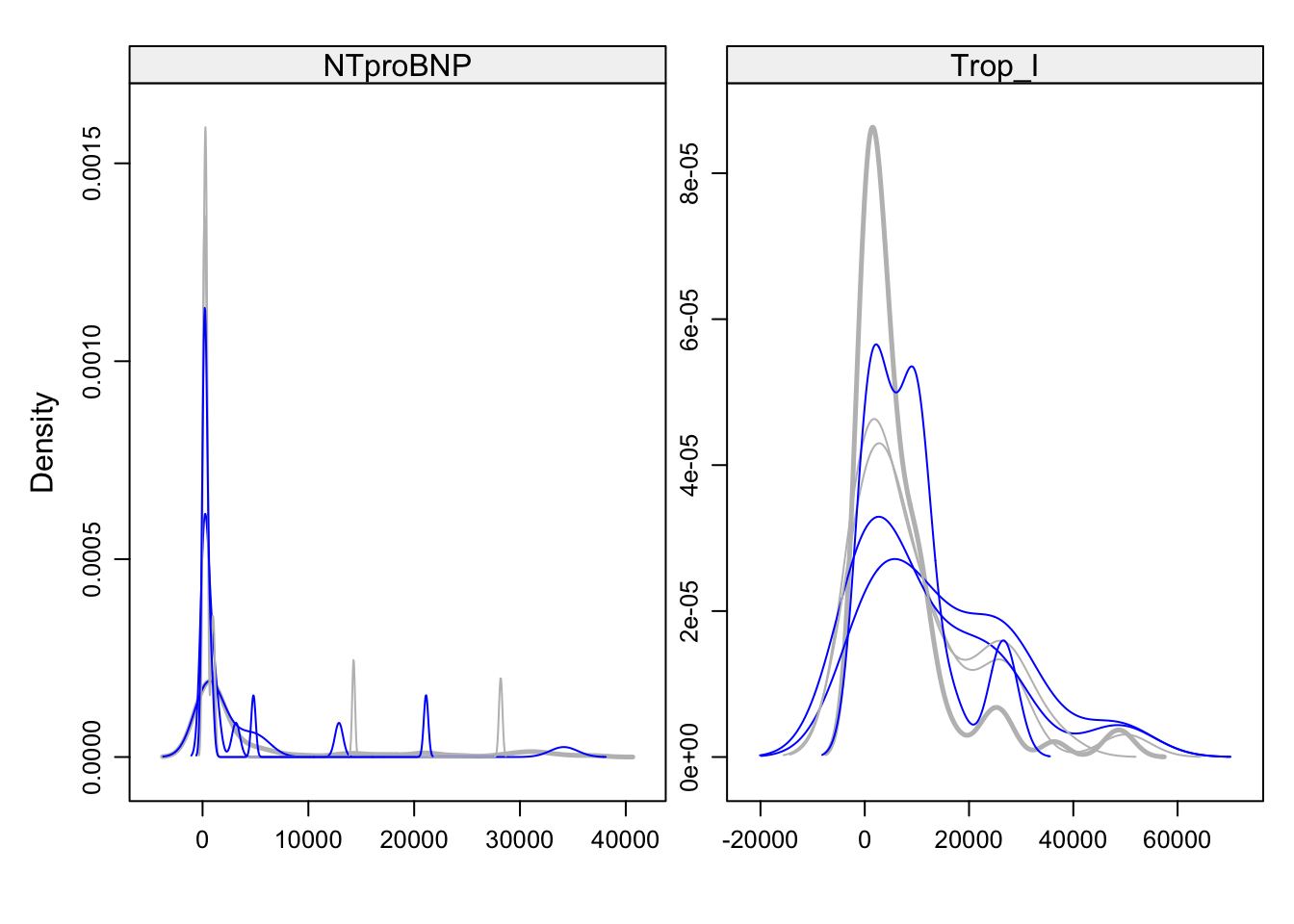
# Create a data set with the observed and completed data
  table_imp <- complete(imputed_data, 1)
Create UMAP and Clustering
# Subset Dataset
  table_umap <- table_imp %>%
                dplyr::select("Study_ID","IL_2R", "HGF", "CXCL9", "CXCL10", "CCL4",
                              "Grem_2", "NTproBNP", "LV_EF")

# Label for Study_ID
  clindat_label <- table_umap[, "Study_ID"]

# Set Study_ID for rownames
  rownames(table_umap) <- table_umap$Study_ID
  table_umap_01 <- subset(table_umap, select= -c(Study_ID))

# Logtranformation
  table_table_umap_log <- log10(table_umap_01)

# Scale
  table_table_umap_log_x <- scale(table_table_umap_log)

# Set seed for reproducibility
  set.seed(100)

# Create UMAP transformation
  umap_clindat <- umap(table_table_umap_log_x)

# Create UMAP data frame
  df_umap_clindat <- data.frame(umap_clindat$layout) %>%
                      tibble::rownames_to_column() %>%
                      rename(Study_ID = rowname)

# Spectral Cluster Analysis
  # Perform spectral clustering
    set.seed(10000)
    spectral_result <- specc(as.matrix(df_umap_clindat[, c("X1", "X2")]), centers = 2)
    df_umap_clindat$cluster <- as.factor(spectral_result@.Data)

# Plot UMAP with Coloring Cluster Annotation Phenotype colors
  plot_umap_clindat <- ggplot(df_umap_clindat,
                       aes(x = X1, y = X2, fill = cluster)) +
                       geom_point(shape = 21, size = 4, color = "black", aes(fill = cluster)) +
                       scale_fill_manual(values = c("2" = "cadetblue4",
                                                    "1" = "plum4")) +
                       labs(title = "Clinical Phenotypes",
                            x = "UMAP1",
                            y = "UMAP2") +
                       theme_classic()

print(plot_umap_clindat) 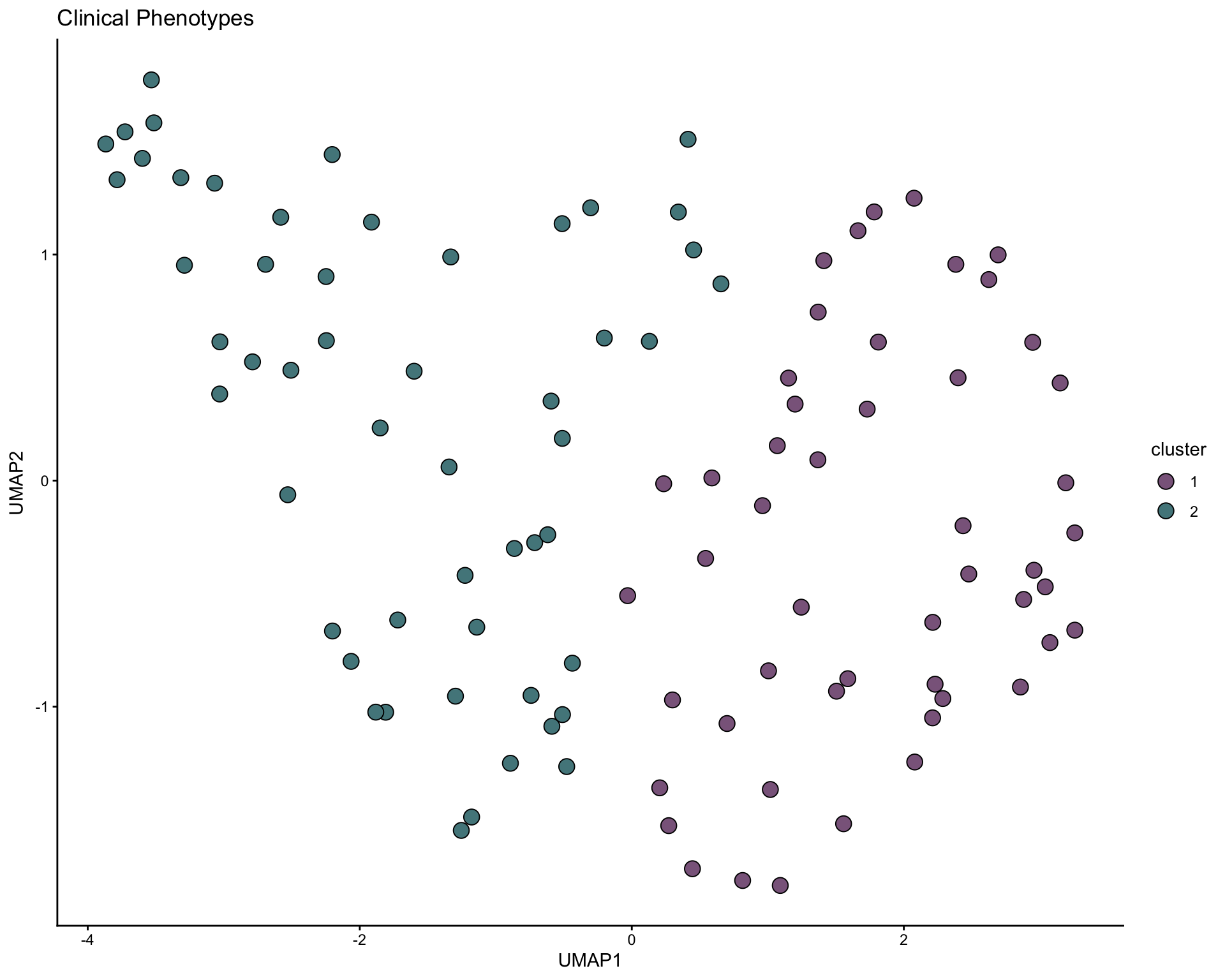
# Plot UMAP with Coloring of Cohort
  df_umap_clindat_cohort <- merge(df_umap_clindat,
                                  data_frame(Study_ID = table_imp$Study_ID, Cohort = table_imp$Cohort) %>%
                                    mutate( Cohort = case_when(
                                            Cohort == "Immpath" ~ "Cohort1",
                                            Cohort == "TUB_Myocarditis" ~ "Cohort2",TRUE ~ Cohort)),by = "Study_ID")

    plot_umap_cohort <- ggplot(df_umap_clindat_cohort,
                             aes(x = X1, y = X2, fill = Cohort)) +
                      geom_point(shape = 21, size = 4, color = "black") +
                      scale_fill_manual(values = c("Cohort1" = "royalblue4",
                                                   "Cohort2" = "orange")) +
                      labs(title = "UMAP: Cohort Distribution",
                           x = "UMAP1",
                           y = "UMAP2",
                           fill = "Cohort") +
                      theme_classic()

print(plot_umap_cohort) 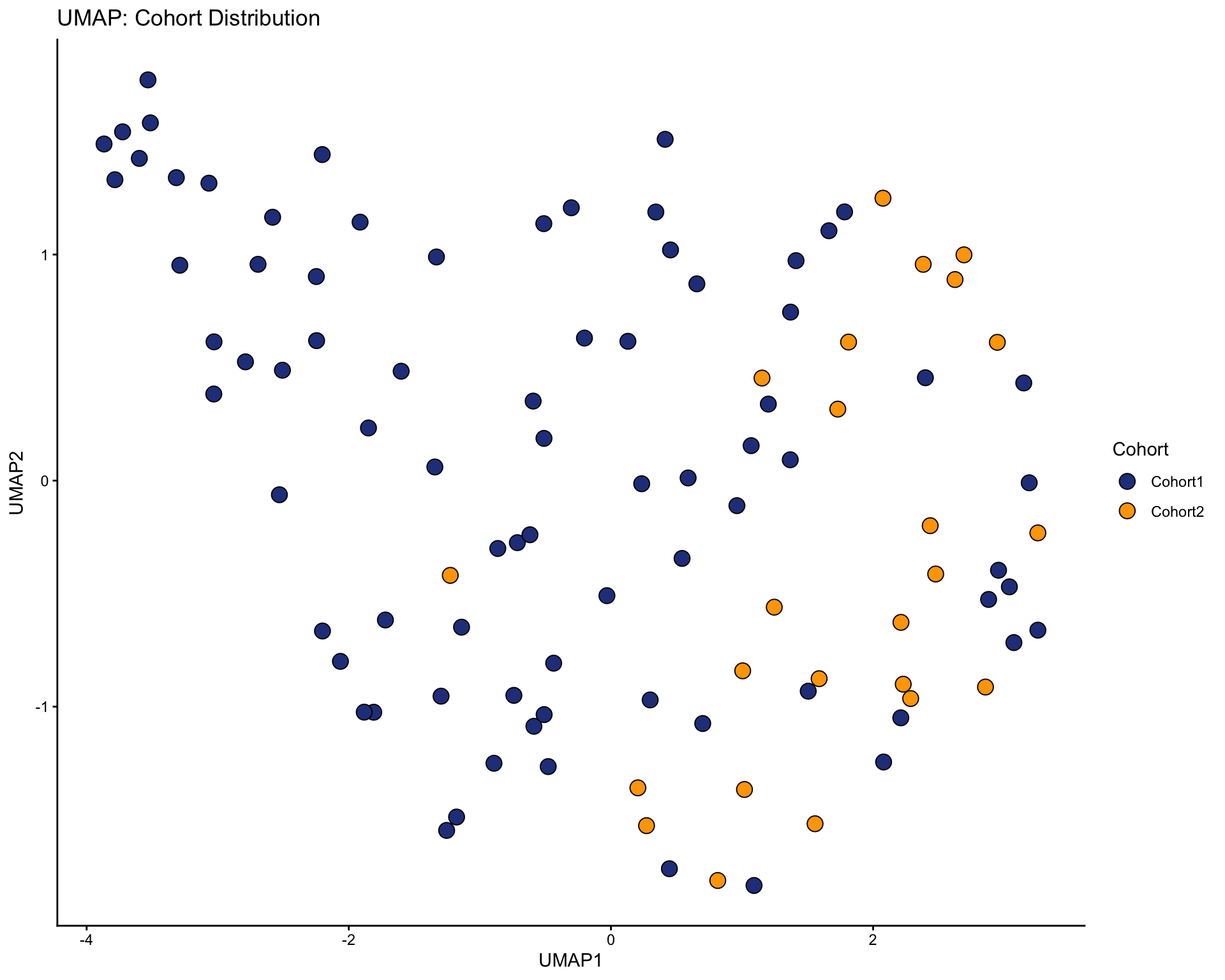
Add Cluster Information
  table_umap_cluster <- merge( table_umap, df_umap_clindat[, c("Study_ID", "cluster")])

# Relabel Cluster
  table_cluster <-  table_umap_cluster %>%
                    mutate(phenotype = case_when(
                           cluster == "2" ~ "Mild",
                           cluster == "1" ~ "Severe",
                           TRUE ~ cluster ))

# Define colors for plots
  cluster_colors <- c("Severe" = "plum4",
                      "Mild" = "cadetblue4")
# Export Table
  write.xlsx(table_cluster, file = file.path(basedir,"data", "Table_phenotypes.xlsx"), row.names = FALSE)
Importance Score using Random Forest
# Set phenotype as Factor with safe names
  table_cluster$phenotype <- factor(table_cluster$phenotype)

# Remove Study_ID
  training_data <- table_cluster %>%
                   dplyr::select(-Study_ID, -cluster)

# Cross Validation
  set.seed(1000)
  control <- trainControl(method = "cv", number = 10, classProbs = TRUE)

# Train Random Forest on imputed data
  rf_imputed <- train(phenotype ~ .,
                      data =  training_data,
                      method = "rf",
                      trControl = control,
                      importance = TRUE,
                      num.trees = 500,
                      maxnodes=4)

# Calculate Accuracy of RF model
  cat("Accuracy:", max(rf_imputed$results$Accuracy), "\n")
Accuracy: 0.8627273 # Show RF variable importance
var_imp <- varImp(rf_imputed, scale = FALSE)
# Caluclate overall importance
varimp <- varImp(rf_imputed, scale = FALSE)$importance
varimp$Overall <- rowMeans(varimp)
head(varimp[order(-varimp$Overall), ]) Mild Severe Overall
Grem_2 11.594889 11.594889 11.594889
LV_EF 11.107213 11.107213 11.107213
CXCL10 10.932231 10.932231 10.932231
HGF 9.567066 9.567066 9.567066
NTproBNP 8.814286 8.814286 8.814286
CXCL9 7.639063 7.639063 7.639063# Plot Top Prediction Variables
imputed_imp <- varImp(rf_imputed, scale = FALSE)
plot_top_pred <- ggplot(imputed_imp, top = 8) +
geom_bar(stat = "identity", width = 0.1) +
ggtitle("Top Predictors - Cluster phenotype") +
theme_bw() +
theme(panel.grid.major = element_blank(),
panel.grid.minor = element_blank())
show(plot_top_pred)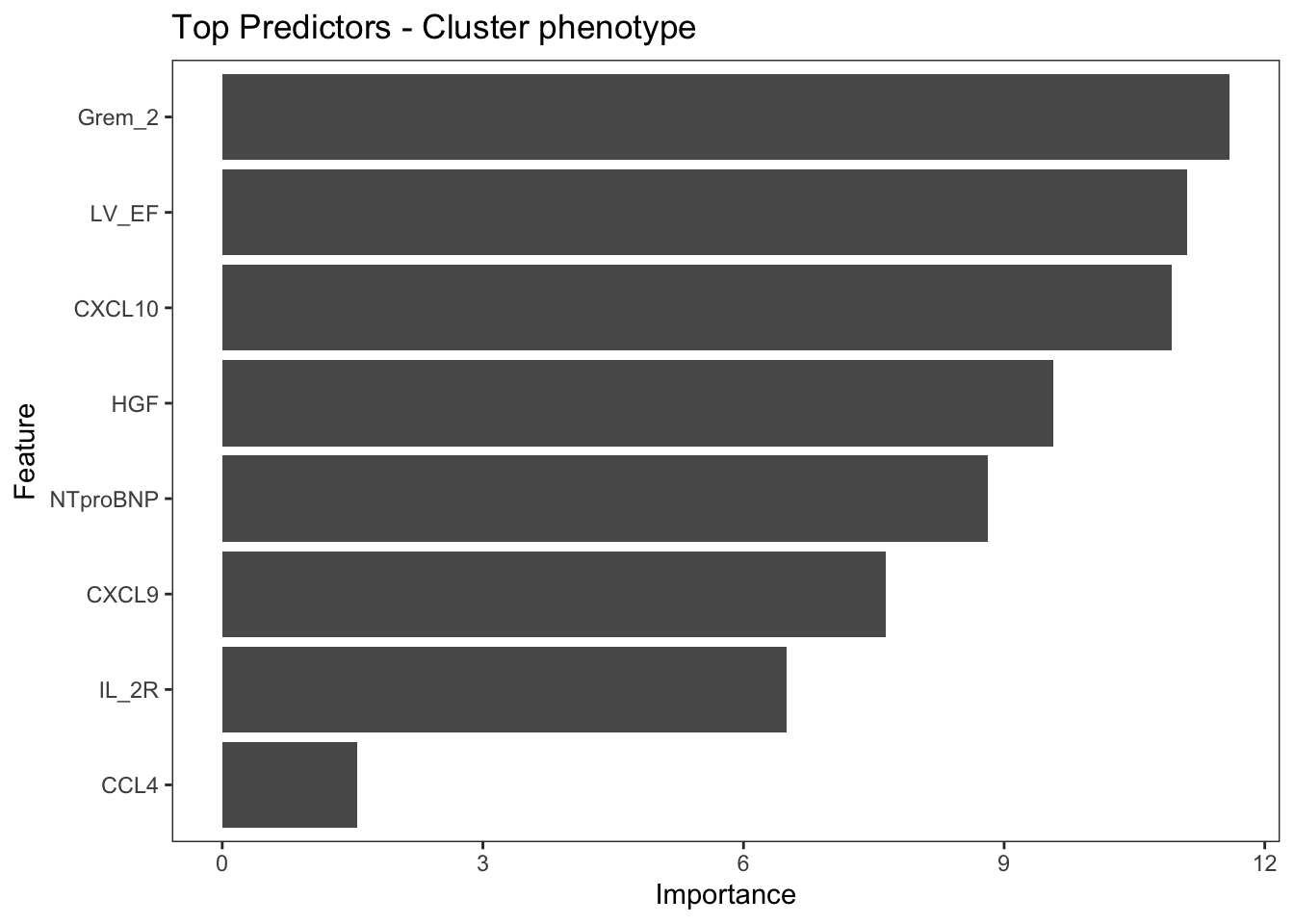
Perform Ridge Regression model detect best predictive parameters for severe and mild
set.seed(100)

# Subset Variables
  table_ridge <-  table_cluster  %>%
                  dplyr::select("Study_ID", "phenotype", "IL_2R", "HGF", "CXCL9", "CXCL10",
                                "CCL4", "Grem_2", "NTproBNP", "LV_EF")

# Log-transform selected biomarkers
  table_ridge <- table_ridge %>%
                 mutate(across(c(IL_2R, HGF, CXCL9, CXCL10, CCL4, Grem_2, LV_EF, NTproBNP), ~ as.numeric(log2(.))))

# Transform phenotype to binary
  table_ridge$phenotype <- factor(table_ridge$phenotype,levels = c("Mild", "Severe"))
  table_ridge$phenotype_binary <- ifelse(table_ridge$phenotype == "Severe", 1, 0)

# Prepare X and y
  X <- model.matrix(phenotype_binary ~ IL_2R + HGF + CXCL9 + CXCL10 + CCL4 + LV_EF + Grem_2 + NTproBNP, table_ridge)[,-1]
  y <- table_ridge$phenotype_binary

# Select optimal lamda
  set.seed(1000)
  ridge_cv <- cv.glmnet(X, y, family = "binomial", alpha = 0, nfolds = 5)
  lambda_min <- ridge_cv$lambda.min

# Fit model
  ridge_model <- glmnet(X, y, family = "binomial", alpha = 0, lambda = lambda_min)

# Estimate p values and CI
  n_boot <- 100

  coef_boot <- matrix(NA, nrow = n_boot, ncol = ncol(X))
  colnames(coef_boot) <- colnames(X)

  for (i in 1:n_boot)

  {
    idx <- sample(1:nrow(table_ridge), replace = TRUE)
    Xb <- X[idx,]
    yb <- y[idx]
    model_b <- glmnet(Xb, yb, family = "binomial", alpha = 0, lambda = lambda_min)
    coef_boot[i, ] <- as.numeric(coef(model_b)[-1])
  }

# Compute mean, 95% CI, and p-value
  coef_mean <- apply(coef_boot, 2, mean)
  coef_low <- apply(coef_boot, 2, function(x) quantile(x, 0.025))
  coef_high <- apply(coef_boot, 2, function(x) quantile(x, 0.975))
  p_values <- 2 * pmin(apply(coef_boot, 2, function(x) mean(x > 0)),
                       apply(coef_boot, 2, function(x) mean(x < 0)))

  table_coef <- data.frame(Predictor = colnames(X),
                          Coefficient = coef_mean,
                          CI_low = coef_low,
                          CI_high = coef_high,
                          p_value = p_values) %>%
                mutate(OR = exp(Coefficient),
                       log_or = log10(OR),
                       log_conf.low = log10(exp(CI_low)),
                       log_conf.high = log10(exp(CI_high)),
                       sig = ifelse(CI_low > 0 | CI_high < 0, "Yes", "No"),
                       color_dir = ifelse(sig == "No", "No", ifelse(log_or < 0, "Left", "Right")),
                       Direction = ifelse(OR > 1, "Severe", "Mild"))

# Plot Forest Plot
# Customize x axis scale
  custom_trans <- trans_new(name = "custom_or",
                  transform = function(x) {ifelse(x < 1, 0.2 * log10(x + 1e-6), 0.2 + 0.8 * log10(x))},
                  inverse = function(x) {ifelse(x < 0.2, 10^(x / 0.2) - 1e-6, 10^((x - 0.2) / 0.8))},
                  domain = c(0, 4))

  plot_forest <-  ggplot(table_coef, aes(y = reorder(Predictor, OR), x = OR, fill = color_dir)) +
                  geom_point(shape = 21, size = 5, color = "black", aes(fill = color_dir)) +
                  geom_errorbarh(aes(xmin = exp(CI_low), xmax = exp(CI_high)), height = 0.2) +
                  geom_vline(xintercept = 1, linetype = "dashed", color = "black") +
                  geom_text(aes(label = paste0(
                                "OR=", round(OR, 2),
                                "\np=", format.pval(p_value, digits = 2, eps = .001)),
                                x = exp(CI_high) * 1.05), size = 3, hjust = 0) +
                  scale_x_continuous(trans = custom_trans,
                                     labels = scales::label_number(accuracy = 0.1),
                                     breaks = c(0.1, 1, 2, 3),)  +
                  scale_fill_manual(values = c("Left" = "cadetblue4", "Right" = "plum4", "No" = "gray")) +
                  theme_classic() +
                  theme(legend.position = "bottom") +
                  labs(title = "Forest Plot Ridge Regression with Bootstrap CI",
                        y = "Predictor",
                        x = "Odds Ratio (95% CI) - per 2x increase in covariante\n
                             Left: favors Mild phenotype, Right: favors Severe phenotype",
                        color = "Direction / Significant")

  print(plot_forest)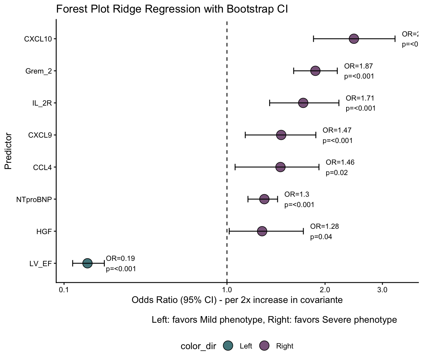
# Summary Table of model
  summary_table <- table_coef %>%
                   mutate(OR = round(OR, 2),
                           CI = paste0(round(exp(CI_low), 2), " - ", round(exp(CI_high), 2)),
                           p_value = ifelse(p_value < 0.001, "< 0.001", signif(p_value, 3))) %>%
                   arrange(desc(OR))%>%
                   dplyr::select(Predictor, OR, CI, p_value)


# Convert summary to table
  table_grob <- gridExtra::tableGrob(summary_table, rows = NULL, theme = gridExtra::ttheme_default(base_size = 10))

# Print table
  combined_plot <- patchwork::wrap_elements(table_grob) + plot_layout(widths = c(2, 1))

  print(combined_plot)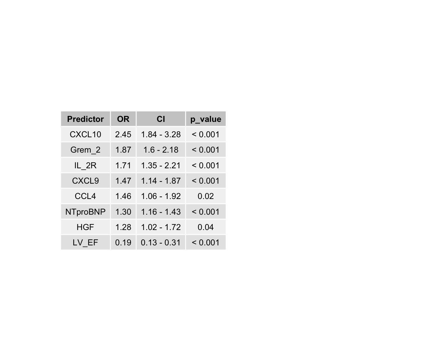
Correlation Plot
# Subset Data table
  table_corr <-  table_cluster  %>%
                 dplyr::select("Study_ID", "phenotype", "IL_2R", "HGF", "CXCL9", "CXCL10",
                               "CCL4", "Grem_2", "NTproBNP", "LV_EF")

# Define colors for plots
  cluster_colors <- c("Severe" = "plum4",
                      "Mild" = "cadetblue4")

# Compute Spearman correlation
  cor_test <- cor.test(table_corr$Grem_2, table_corr$LV_EF, method = "spearman")

  plot <-   ggplot(table_corr, aes(y = LV_EF, x = Grem_2, color = phenotype)) +
            geom_point(aes(fill = phenotype, size = CXCL10),
                           shape = 21, color = "black", alpha = 0.8) +
            scale_size_continuous(name = "CXCL10 (pg/ml)",
                                  range = c(2, 15),
                                  breaks = c(35, 50, 100),
                                  labels = c("35", "50", "100"),
                                  limits = c(35, 600)) +
            geom_smooth(method = "lm", se = TRUE, color = "black") +
            scale_fill_manual(values = cluster_colors)  +
            scale_x_log10(labels = function(y) format(y, scientific = FALSE, trim = TRUE),
                          breaks = c(300, 1000, 3000, 10000, 35000),
                          limits = c(300,35000))  +
            scale_y_continuous(limits = c(0,75),
                               breaks = c(25, 50, 75),
                               expand = c(0, 0)) +
            theme_classic() +
            labs(y = "LVEF (%)", x = "Gremlin-2 (pg/ml)") +
            annotate("text",
                     y = min(table_corr$LV_EF, na.rm = TRUE),
                     x = max(table_corr$Grem_2, na.rm = TRUE),
                     label = paste0("r = ", round(cor_test$estimate, 2),
                                    "\np = ", ifelse(cor_test$p.value < 0.001, "< 0.001",
                                                     signif(cor_test$p.value, 3))),
                     hjust = 1,vjust = 1, size = 5) +
            scale_color_manual(values = cluster_colors) +
            coord_cartesian(clip = "off")

  print(plot)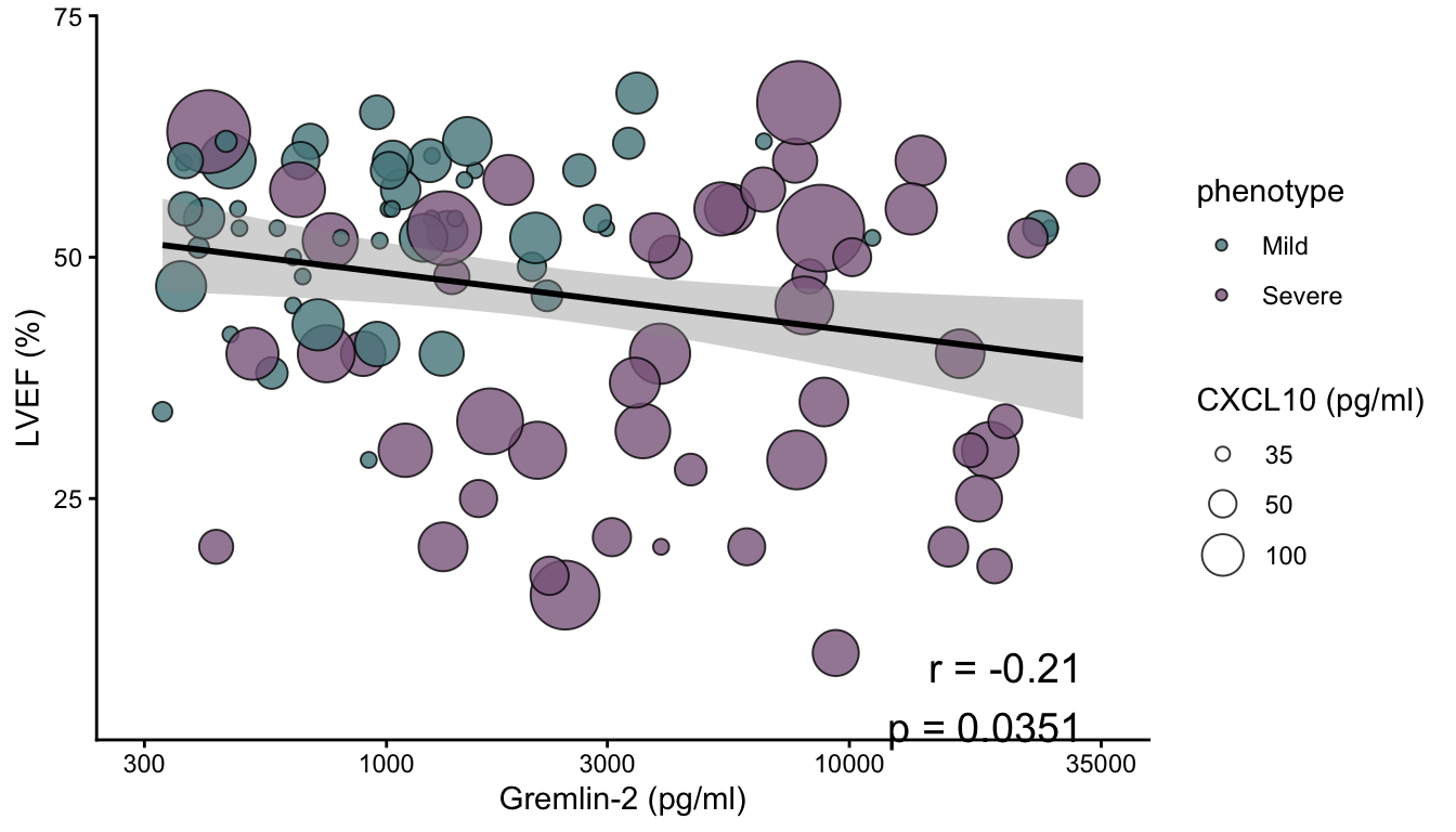
Roc Curve
# Data preparation
  table_roc <- table_cluster %>%
               dplyr::select(Study_ID, phenotype, CXCL10, Grem_2, LV_EF) %>%
               mutate(phenotype = factor(phenotype, levels = c("Mild", "Severe")),
                      outcome_binary = ifelse(phenotype == "Severe", 1, 0))

# Select predictors
  param <- c("CXCL10", "Grem_2", "LV_EF")
  biomarker_labels <- c(CXCL10 = "CXCL10", Grem_2 = "Gremlin-2", LV_EF = "LVEF", Combined = "Combined model")

# Initialize storage
  roc_list <- list()

# Create ROC Curve for each parameter
  for (p in param)

  {
    roc_obj <- roc(response = table_roc$outcome_binary,
                   predictor = table_roc[[p]],
                   levels = c(0, 1),
                   direction = "auto",
                   ci = TRUE,
                   legacy.axes = TRUE)

    roc_list[[p]] <- roc_obj
  }

# Create ROC Curve for comined model

  # Create formula dynamically
    formula_str <- paste("outcome_binary ~", paste(param, collapse = " + "))

    model <- glm(as.formula(formula_str),
                 data = table_roc,
                 family = binomial)

    summary(model)
Call:
glm(formula = as.formula(formula_str), family = binomial, data = table_roc)

Coefficients:
              Estimate Std. Error z value Pr(>|z|)
(Intercept)  1.729e+00  1.522e+00   1.136 0.255979
CXCL10       3.989e-02  9.423e-03   4.233 2.30e-05 ***
Grem_2       1.830e-04  5.502e-05   3.325 0.000883 ***
LV_EF       -1.442e-01  3.665e-02  -3.935 8.31e-05 ***
---
Signif. codes:  0 '***' 0.001 '**' 0.01 '*' 0.05 '.' 0.1 ' ' 1

(Dispersion parameter for binomial family taken to be 1)

    Null deviance: 142.701  on 102  degrees of freedom
Residual deviance:  51.087  on  99  degrees of freedom
AIC: 59.087

Number of Fisher Scoring iterations: 8
# Predicted probabilities (prob of being Severe)
predictions <- predict(model, type = "response")
# Compute ROC curve for combined model
roc_combined <- roc(response = table_roc$outcome_binary,
predictor = predictions,
levels = c(0, 1),
direction = "<",
ci = TRUE)
roc_list[["Combined"]] <- roc_combined
# AUC & CI values
auc_vals <- sapply(roc_list, function(x) as.numeric(auc(x)))
auc_ci <- lapply(roc_list, function(x) ci.auc(x))
# Create Legend
legend_text <- mapply(function(name, auc, ci) {
paste0(biomarker_labels[name],
" (AUC = ", round(auc,2),
", 95% CI: ", round(ci[1],2),
"–", round(ci[3],2), ")")},
names(roc_list), auc_vals,auc_ci)
# Combine ROC curves into ggplot
roc_plot <- ggroc(roc_list, legacy.axes = TRUE) +
geom_abline(intercept = 0, slope = 1, linetype = "dashed", color = "grey") +
scale_color_manual(values = c("lightblue", "lightblue4", "darkgrey", "plum4"),
labels = legend_text) +
theme_classic() +
theme(panel.border = element_rect(color = "black", fill = NA, linewidth = 1),
legend.position = "bottom",
legend.direction = "vertical") +
labs(x = "1 - Specificity",
y = "Sensitivity",
color = "Legend") +
coord_equal()
print(roc_plot)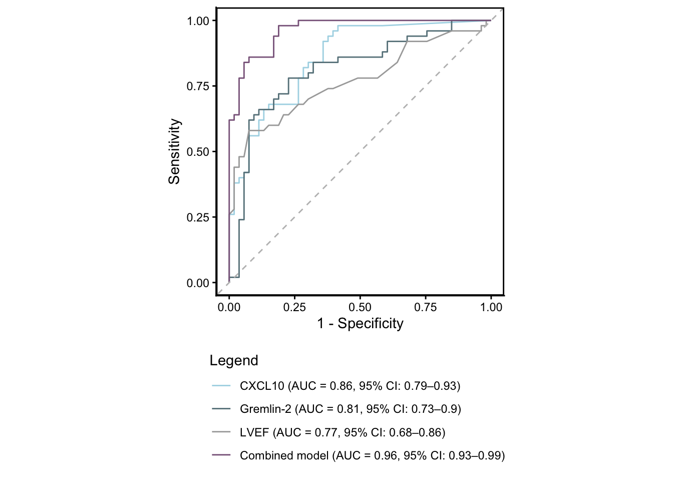
session info
sessionInfo()R version 4.4.3 (2025-02-28)
Platform: aarch64-apple-darwin20
Running under: macOS 26.3
Matrix products: default
BLAS: /Library/Frameworks/R.framework/Versions/4.4-arm64/Resources/lib/libRblas.0.dylib
LAPACK: /Library/Frameworks/R.framework/Versions/4.4-arm64/Resources/lib/libRlapack.dylib; LAPACK version 3.12.0
locale:
[1] en_US.UTF-8/en_US.UTF-8/en_US.UTF-8/C/en_US.UTF-8/en_US.UTF-8
time zone: Europe/Zurich
tzcode source: internal
attached base packages:
[1] grid stats graphics grDevices utils datasets methods
[8] base
other attached packages:
[1] ImmunoLogic_0.0.0.9000 Seurat_5.3.1 SeuratObject_5.2.0
[4] sp_2.2-0 kernlab_0.9-33 dbscan_1.2-0
[7] umap_0.2.10.0 Rtsne_0.17 cluster_2.1.8
[10] factoextra_1.0.7 randomForest_4.7-1.2 pROC_1.19.0.1
[13] mice_3.18.0 caret_7.0-1 lattice_0.22-6
[16] drc_3.0-1 logistf_1.26.1 glmnet_4.1-10
[19] Matrix_1.7-2 broom_1.0.11 MuMIn_1.48.11
[22] Hmisc_5.2-3 car_3.1-3 carData_3.0-5
[25] multcomp_1.4-28 TH.data_1.1-4 MASS_7.3-65
[28] survival_3.8-3 mvtnorm_1.3-3 rstatix_0.7.3
[31] ggpattern_1.2.1 gridExtra_2.3 cowplot_1.2.0
[34] patchwork_1.3.2 plotly_4.11.0 EnhancedVolcano_1.24.0
[37] RColorBrewer_1.1-3 circlize_0.4.16 ComplexHeatmap_2.22.0
[40] pheatmap_1.0.12 corrplot_0.95 ggcorrplot_0.1.4.1
[43] ggbeeswarm_0.7.2 ggrepel_0.9.6 ggpubr_0.6.2
[46] readxl_1.4.5 writexl_1.5.0 openxlsx_4.2.5.2
[49] gtsummary_2.4.0 flextable_0.9.6 tableone_0.13.2
[52] table1_1.4.3 scales_1.4.0 here_1.0.2
[55] janitor_2.2.0 magrittr_2.0.4 data.table_1.17.8
[58] lubridate_1.9.4 forcats_1.0.1 stringr_1.6.0
[61] dplyr_1.1.4 purrr_1.2.0 readr_2.1.6
[64] tidyr_1.3.1 tibble_3.3.0 ggplot2_4.0.1
[67] tidyverse_2.0.0
loaded via a namespace (and not attached):
[1] IRanges_2.40.1 nnet_7.3-20 goftest_1.2-3
[4] vctrs_0.6.5 spatstat.random_3.4-3 proxy_0.4-27
[7] digest_0.6.39 png_0.1-8 shape_1.4.6.1
[10] git2r_0.36.2 alabama_2023.1.0 deldir_2.0-4
[13] httpcode_0.3.0 parallelly_1.45.1 fontLiberation_0.1.0
[16] reshape2_1.4.5 httpuv_1.6.16 foreach_1.5.2
[19] BiocGenerics_0.52.0 withr_3.0.2 xfun_0.54
[22] crul_1.4.2 emmeans_1.10.4 systemfonts_1.3.1
[25] ragg_1.5.0 zoo_1.8-14 GlobalOptions_0.1.3
[28] gtools_3.9.5 pbapply_1.7-4 Formula_1.2-5
[31] promises_1.5.0 otel_0.2.0 httr_1.4.7
[34] globals_0.18.0 fitdistrplus_1.2-4 rstudioapi_0.17.1
[37] pan_1.9 miniUI_0.1.2 generics_0.1.4
[40] base64enc_0.1-3 curl_7.0.0 S4Vectors_0.44.0
[43] mitools_2.4 polyclip_1.10-7 quadprog_1.5-8
[46] xtable_1.8-4 doParallel_1.0.17 evaluate_1.0.5
[49] hms_1.1.4 irlba_2.3.5.1 colorspace_2.1-2
[52] polynom_1.4-1 ROCR_1.0-11 reticulate_1.44.1
[55] spatstat.data_3.1-9 lmtest_0.9-40 snakecase_0.11.1
[58] later_1.4.4 spatstat.geom_3.6-1 future.apply_1.20.0
[61] scattermore_1.2 survey_4.4-2 matrixStats_1.5.0
[64] RcppAnnoy_0.0.22 class_7.3-23 pillar_1.11.1
[67] nlme_3.1-167 iterators_1.0.14 compiler_4.4.3
[70] RSpectra_0.16-2 stringi_1.8.7 gower_1.0.2
[73] jomo_2.7-6 tensor_1.5.1 minqa_1.2.8
[76] plyr_1.8.9 crayon_1.5.3 abind_1.4-8
[79] orthopolynom_1.0-6.1 sandwich_3.1-1 whisker_0.4.1
[82] codetools_0.2-20 textshaping_1.0.4 basefun_1.2-4
[85] recipes_1.3.1 openssl_2.3.4 bslib_0.9.0
[88] e1071_1.7-14 GetoptLong_1.0.5 mime_0.13
[91] splines_4.4.3 Rcpp_1.1.0 fastDummies_1.7.5
[94] coneproj_1.20 variables_1.1-2 cellranger_1.1.0
[97] knitr_1.50 clue_0.3-66 lme4_1.1-38
[100] fs_1.6.6 listenv_0.10.0 checkmate_2.3.3
[103] Rdpack_2.6.4 ggsignif_0.6.4 estimability_1.5.1
[106] tzdb_0.5.0 pkgconfig_2.0.3 tools_4.4.3
[109] cachem_1.1.0 rbibutils_2.4 numDeriv_2016.8-1.1
[112] viridisLite_0.4.2 DBI_1.2.3 fastmap_1.2.0
[115] rmarkdown_2.30 ica_1.0-3 tram_1.2-4
[118] sass_0.4.10 officer_0.6.6 coda_0.19-4.1
[121] dotCall64_1.2 RANN_2.6.2 rpart_4.1.24
[124] farver_2.1.2 reformulas_0.4.2 mgcv_1.9-1
[127] yaml_2.3.11 workflowr_1.7.2 foreign_0.8-88
[130] cli_3.6.5 stats4_4.4.3 lifecycle_1.0.4
[133] uwot_0.2.4 askpass_1.2.1 lava_1.8.0
[136] backports_1.5.0 mlt_1.6-6 timechange_0.3.0
[139] gtable_0.3.6 rjson_0.2.23 ggridges_0.5.7
[142] progressr_0.18.0 parallel_4.4.3 jsonlite_2.0.0
[145] RcppHNSW_0.6.0 mitml_0.4-5 qrng_0.0-10
[148] spatstat.utils_3.2-0 zip_2.3.1 jquerylib_0.1.4
[151] spatstat.univar_3.1-5 timeDate_4051.111 lazyeval_0.2.2
[154] shiny_1.12.0 htmltools_0.5.9 sctransform_0.4.2
[157] glue_1.8.0 gfonts_0.2.0 BB_2019.10-1
[160] spam_2.11-1 gdtools_0.3.7 rprojroot_2.1.1
[163] boot_1.3-31 igraph_2.2.1 R6_2.6.1
[166] labeling_0.4.3 ipred_0.9-15 nloptr_2.2.1
[169] tidyselect_1.2.1 vipor_0.4.7 plotrix_3.8-4
[172] htmlTable_2.4.3 operator.tools_1.6.3 xml2_1.5.1
[175] fontBitstreamVera_0.1.1 future_1.68.0 ModelMetrics_1.2.2.2
[178] KernSmooth_2.23-26 S7_0.2.1 fontquiver_0.2.1
[181] htmlwidgets_1.6.4 rlang_1.1.6 spatstat.sparse_3.1-0
[184] spatstat.explore_3.6-0 uuid_1.2-1 formula.tools_1.7.1
[187] hardhat_1.4.1 beeswarm_0.4.0 prodlim_2023.08.28 date()[1] "Fri Mar 6 19:19:35 2026"
sessionInfo()R version 4.4.3 (2025-02-28)
Platform: aarch64-apple-darwin20
Running under: macOS 26.3
Matrix products: default
BLAS: /Library/Frameworks/R.framework/Versions/4.4-arm64/Resources/lib/libRblas.0.dylib
LAPACK: /Library/Frameworks/R.framework/Versions/4.4-arm64/Resources/lib/libRlapack.dylib; LAPACK version 3.12.0
locale:
[1] en_US.UTF-8/en_US.UTF-8/en_US.UTF-8/C/en_US.UTF-8/en_US.UTF-8
time zone: Europe/Zurich
tzcode source: internal
attached base packages:
[1] grid stats graphics grDevices utils datasets methods
[8] base
other attached packages:
[1] ImmunoLogic_0.0.0.9000 Seurat_5.3.1 SeuratObject_5.2.0
[4] sp_2.2-0 kernlab_0.9-33 dbscan_1.2-0
[7] umap_0.2.10.0 Rtsne_0.17 cluster_2.1.8
[10] factoextra_1.0.7 randomForest_4.7-1.2 pROC_1.19.0.1
[13] mice_3.18.0 caret_7.0-1 lattice_0.22-6
[16] drc_3.0-1 logistf_1.26.1 glmnet_4.1-10
[19] Matrix_1.7-2 broom_1.0.11 MuMIn_1.48.11
[22] Hmisc_5.2-3 car_3.1-3 carData_3.0-5
[25] multcomp_1.4-28 TH.data_1.1-4 MASS_7.3-65
[28] survival_3.8-3 mvtnorm_1.3-3 rstatix_0.7.3
[31] ggpattern_1.2.1 gridExtra_2.3 cowplot_1.2.0
[34] patchwork_1.3.2 plotly_4.11.0 EnhancedVolcano_1.24.0
[37] RColorBrewer_1.1-3 circlize_0.4.16 ComplexHeatmap_2.22.0
[40] pheatmap_1.0.12 corrplot_0.95 ggcorrplot_0.1.4.1
[43] ggbeeswarm_0.7.2 ggrepel_0.9.6 ggpubr_0.6.2
[46] readxl_1.4.5 writexl_1.5.0 openxlsx_4.2.5.2
[49] gtsummary_2.4.0 flextable_0.9.6 tableone_0.13.2
[52] table1_1.4.3 scales_1.4.0 here_1.0.2
[55] janitor_2.2.0 magrittr_2.0.4 data.table_1.17.8
[58] lubridate_1.9.4 forcats_1.0.1 stringr_1.6.0
[61] dplyr_1.1.4 purrr_1.2.0 readr_2.1.6
[64] tidyr_1.3.1 tibble_3.3.0 ggplot2_4.0.1
[67] tidyverse_2.0.0
loaded via a namespace (and not attached):
[1] IRanges_2.40.1 nnet_7.3-20 goftest_1.2-3
[4] vctrs_0.6.5 spatstat.random_3.4-3 proxy_0.4-27
[7] digest_0.6.39 png_0.1-8 shape_1.4.6.1
[10] git2r_0.36.2 alabama_2023.1.0 deldir_2.0-4
[13] httpcode_0.3.0 parallelly_1.45.1 fontLiberation_0.1.0
[16] reshape2_1.4.5 httpuv_1.6.16 foreach_1.5.2
[19] BiocGenerics_0.52.0 withr_3.0.2 xfun_0.54
[22] crul_1.4.2 emmeans_1.10.4 systemfonts_1.3.1
[25] ragg_1.5.0 zoo_1.8-14 GlobalOptions_0.1.3
[28] gtools_3.9.5 pbapply_1.7-4 Formula_1.2-5
[31] promises_1.5.0 otel_0.2.0 httr_1.4.7
[34] globals_0.18.0 fitdistrplus_1.2-4 rstudioapi_0.17.1
[37] pan_1.9 miniUI_0.1.2 generics_0.1.4
[40] base64enc_0.1-3 curl_7.0.0 S4Vectors_0.44.0
[43] mitools_2.4 polyclip_1.10-7 quadprog_1.5-8
[46] xtable_1.8-4 doParallel_1.0.17 evaluate_1.0.5
[49] hms_1.1.4 irlba_2.3.5.1 colorspace_2.1-2
[52] polynom_1.4-1 ROCR_1.0-11 reticulate_1.44.1
[55] spatstat.data_3.1-9 lmtest_0.9-40 snakecase_0.11.1
[58] later_1.4.4 spatstat.geom_3.6-1 future.apply_1.20.0
[61] scattermore_1.2 survey_4.4-2 matrixStats_1.5.0
[64] RcppAnnoy_0.0.22 class_7.3-23 pillar_1.11.1
[67] nlme_3.1-167 iterators_1.0.14 compiler_4.4.3
[70] RSpectra_0.16-2 stringi_1.8.7 gower_1.0.2
[73] jomo_2.7-6 tensor_1.5.1 minqa_1.2.8
[76] plyr_1.8.9 crayon_1.5.3 abind_1.4-8
[79] orthopolynom_1.0-6.1 sandwich_3.1-1 whisker_0.4.1
[82] codetools_0.2-20 textshaping_1.0.4 basefun_1.2-4
[85] recipes_1.3.1 openssl_2.3.4 bslib_0.9.0
[88] e1071_1.7-14 GetoptLong_1.0.5 mime_0.13
[91] splines_4.4.3 Rcpp_1.1.0 fastDummies_1.7.5
[94] coneproj_1.20 variables_1.1-2 cellranger_1.1.0
[97] knitr_1.50 clue_0.3-66 lme4_1.1-38
[100] fs_1.6.6 listenv_0.10.0 checkmate_2.3.3
[103] Rdpack_2.6.4 ggsignif_0.6.4 estimability_1.5.1
[106] tzdb_0.5.0 pkgconfig_2.0.3 tools_4.4.3
[109] cachem_1.1.0 rbibutils_2.4 numDeriv_2016.8-1.1
[112] viridisLite_0.4.2 DBI_1.2.3 fastmap_1.2.0
[115] rmarkdown_2.30 ica_1.0-3 tram_1.2-4
[118] sass_0.4.10 officer_0.6.6 coda_0.19-4.1
[121] dotCall64_1.2 RANN_2.6.2 rpart_4.1.24
[124] farver_2.1.2 reformulas_0.4.2 mgcv_1.9-1
[127] yaml_2.3.11 workflowr_1.7.2 foreign_0.8-88
[130] cli_3.6.5 stats4_4.4.3 lifecycle_1.0.4
[133] uwot_0.2.4 askpass_1.2.1 lava_1.8.0
[136] backports_1.5.0 mlt_1.6-6 timechange_0.3.0
[139] gtable_0.3.6 rjson_0.2.23 ggridges_0.5.7
[142] progressr_0.18.0 parallel_4.4.3 jsonlite_2.0.0
[145] RcppHNSW_0.6.0 mitml_0.4-5 qrng_0.0-10
[148] spatstat.utils_3.2-0 zip_2.3.1 jquerylib_0.1.4
[151] spatstat.univar_3.1-5 timeDate_4051.111 lazyeval_0.2.2
[154] shiny_1.12.0 htmltools_0.5.9 sctransform_0.4.2
[157] glue_1.8.0 gfonts_0.2.0 BB_2019.10-1
[160] spam_2.11-1 gdtools_0.3.7 rprojroot_2.1.1
[163] boot_1.3-31 igraph_2.2.1 R6_2.6.1
[166] labeling_0.4.3 ipred_0.9-15 nloptr_2.2.1
[169] tidyselect_1.2.1 vipor_0.4.7 plotrix_3.8-4
[172] htmlTable_2.4.3 operator.tools_1.6.3 xml2_1.5.1
[175] fontBitstreamVera_0.1.1 future_1.68.0 ModelMetrics_1.2.2.2
[178] KernSmooth_2.23-26 S7_0.2.1 fontquiver_0.2.1
[181] htmlwidgets_1.6.4 rlang_1.1.6 spatstat.sparse_3.1-0
[184] spatstat.explore_3.6-0 uuid_1.2-1 formula.tools_1.7.1
[187] hardhat_1.4.1 beeswarm_0.4.0 prodlim_2023.08.28