Differential Gene Expression using DEseq2
Maeva Techer
2022-11-01
Last updated: 2022-11-01
Checks: 6 1
Knit directory:
locust-phase-transition-RNAseq/
This reproducible R Markdown analysis was created with workflowr (version 1.7.0). The Checks tab describes the reproducibility checks that were applied when the results were created. The Past versions tab lists the development history.
Great! Since the R Markdown file has been committed to the Git repository, you know the exact version of the code that produced these results.
Great job! The global environment was empty. Objects defined in the global environment can affect the analysis in your R Markdown file in unknown ways. For reproduciblity it’s best to always run the code in an empty environment.
The command set.seed(20221025) was run prior to running
the code in the R Markdown file. Setting a seed ensures that any results
that rely on randomness, e.g. subsampling or permutations, are
reproducible.
Great job! Recording the operating system, R version, and package versions is critical for reproducibility.
Nice! There were no cached chunks for this analysis, so you can be confident that you successfully produced the results during this run.
Using absolute paths to the files within your workflowr project makes it difficult for you and others to run your code on a different machine. Change the absolute path(s) below to the suggested relative path(s) to make your code more reproducible.
| absolute | relative |
|---|---|
| /Users/alphamanae/Documents/GitHub/locust-phase-transition-RNAseq | . |
| /Users/alphamanae/Documents/GitHub/locust-phase-transition-RNAseq/data/piceifrons | data/piceifrons |
| /Users/alphamanae/Documents/GitHub/locust-phase-transition-RNAseq/data/piceifrons/STAR_counts_4thcol | data/piceifrons/STAR_counts_4thcol |
| /Users/alphamanae/Documents/GitHub/locust-phase-transition-RNAseq/data/piceifrons/list/HeadSPICE.txt | data/piceifrons/list/HeadSPICE.txt |
Great! You are using Git for version control. Tracking code development and connecting the code version to the results is critical for reproducibility.
The results in this page were generated with repository version a1837b0. See the Past versions tab to see a history of the changes made to the R Markdown and HTML files.
Note that you need to be careful to ensure that all relevant files for
the analysis have been committed to Git prior to generating the results
(you can use wflow_publish or
wflow_git_commit). workflowr only checks the R Markdown
file, but you know if there are other scripts or data files that it
depends on. Below is the status of the Git repository when the results
were generated:
Ignored files:
    Ignored:    .DS_Store
    Ignored:    analysis/.DS_Store
    Ignored:    data/.DS_Store
    Ignored:    data/americana/.DS_Store
    Ignored:    data/americana/STAR_counts_4thcol/.DS_Store
    Ignored:    data/cancellata/.DS_Store
    Ignored:    data/cancellata/STAR_counts_4thcol/.DS_Store
    Ignored:    data/cubense/.DS_Store
    Ignored:    data/cubense/STAR_counts_4thcol/.DS_Store
    Ignored:    data/gregaria/.DS_Store
    Ignored:    data/gregaria/STAR_counts_4thcol/.DS_Store
    Ignored:    data/gregaria/list/.DS_Store
    Ignored:    data/metadata/.DS_Store
    Ignored:    data/nitens/.DS_Store
    Ignored:    data/nitens/STAR_counts_4thcol/.DS_Store
    Ignored:    data/piceifrons/.DS_Store
    Ignored:    data/piceifrons/DEseq2_SPICE_HEAD/.DS_Store
    Ignored:    data/piceifrons/STAR_counts_4thcol/.DS_Store
    Ignored:    data/piceifrons/edgeR_SPICE_HEAD/.DS_Store
    Ignored:    data/piceifrons/list/.DS_Store

Untracked files:
    Untracked:  data/piceifrons/DE-genes_strict_[SPICE_HEAD]_[238_genes].txt
    Untracked:  data/piceifrons/DEseq2_SPICE_HEAD/DE-genes_[SPICE_HEAD_DEseq2]_[378_genes].txt
    Untracked:  data/piceifrons/edgeR_SPICE_HEAD/DE-genes_[SPICE_HEAD_edgeR]_[342_genes].txt
Note that any generated files, e.g. HTML, png, CSS, etc., are not included in this status report because it is ok for generated content to have uncommitted changes.
These are the previous versions of the repository in which changes were
made to the R Markdown (analysis/deseq2-workflow.Rmd) and
HTML (docs/deseq2-workflow.html) files. If you’ve
configured a remote Git repository (see ?wflow_git_remote),
click on the hyperlinks in the table below to view the files as they
were in that past version.
| File | Version | Author | Date | Message |
|---|---|---|---|---|
| html | 83b00b8 | MaevaTecher | 2022-11-01 | Build site. |
| html | 05f27e6 | MaevaTecher | 2022-11-01 | Build site. |
| Rmd | 125349f | MaevaTecher | 2022-11-01 | adding DEseq and EdgeR analysis |
| html | 125349f | MaevaTecher | 2022-11-01 | adding DEseq and EdgeR analysis |
Load required R libraries
#(install first from CRAN or Bioconductor)
library("knitr")
library("rmdformats")
library("tidyverse")
library("DT")  # for making interactive search table
library("plotly") # for interactive plots
library("ggthemes") # for theme_calc
library("reshape2")
library("DESeq2")
library("data.table")
library("apeglm")
library("ggpubr")
library("ggplot2")
library("ggrepel")
library("EnhancedVolcano")
library("SARTools")
library("pheatmap")

## Global options
options(max.print="10000")
knitr::opts_chunk$set(
    echo = TRUE,
    message = FALSE,
    warning = FALSE,
    cache = FALSE,
    comment = FALSE,
    prompt = FALSE,
    tidy = TRUE
)
opts_knit$set(width=75)
Here we present the workflow example with the head data from S. piceifrons
For the analysis of differentially expressed genes, we will follow
some guidelines from an online RNA course tutorial
that uses either DESeq2 or edgeR on STAR
output. We also adapted some script lines from Foquet et al. 2021
code.
DESeq2 tests for differential expression using negative binomial generalized linear models. DESeq2 (as edgeR) is based on the hypothesis that most genes are not differentially expressed. The package takes as an input raw counts (i.e. non normalized counts): the DESeq2 model internally corrects for library size, so giving as an input normalized count would be incorrect.
DESeq2 analysis using STAR input
Preparing input files
Raw count matrices
We generated this in the precedent section.
Transcript-to-gene annotation file
Below is the example with S. piceifrons
# Download annotation and place it into the folder refgenomes
wget https://ftp.ncbi.nlm.nih.gov/genomes/all/GCF/021/461/385/GCF_021461385.2_iqSchPice1.1/GCF_021461385.2_iqSchPice1.1_genomic.gtf.gz

# first column is the transcript ID, second column is the gene ID, third column is the gene symbol
zcat GCF_021461385.2_iqSchPice1.1_genomic.gtf.gz | awk -F "\t" 'BEGIN{OFS="\t"}{if($3=="transcript"){split($9, a, "\""); print a[4],a[2],a[8]}}' > tx2gene.piceifrons.csv
Sample sheet
DESeq2 needs a sample sheet that describes the samples characteristics: SampleName, FileName (…counts.txt), and subsequently anything that can be used for statistical design such as RearingCondition, replicates, tissue, time points, etc. in the form.
The design indicates how to model the samples: in the model we need to specify what we want to measure and what we want to control.
Differential expression analysis
Import input count data
We start by reading the sample sheet.
############################### MOSTLY FOR THE HMTL REPORT PARAMETERS for
############################### running the script
homeDir <- "/Users/alphamanae/Documents/GitHub/locust-phase-transition-RNAseq"
workDir <- "/Users/alphamanae/Documents/GitHub/locust-phase-transition-RNAseq/data/piceifrons"  # Working directory
projectName <- "SPICE_HEAD"  # name of the project
author <- "Maeva TECHER"  # author of the statistical analysis/report

## Create all the needed directories
setwd(workDir)
Dirname <- paste("DEseq2_", projectName, sep = "")
dir.create(Dirname)
setwd(Dirname)
workDir_DEseq2 <- getwd()
# path to the directory containing raw counts files
rawDir <- "/Users/alphamanae/Documents/GitHub/locust-phase-transition-RNAseq/data/piceifrons/STAR_counts_4thcol"

## PARAMETERS for running DEseq2
tresh_logfold <- 1  # Treshold for log2(foldchange) in final DE-files
tresh_padj <- 0.05  # Treshold for adjusted p-valued in final DE-files
alpha_DEseq2 <- 0.05  # threshold of statistical significance
pAdjustMethod_DEseq2 <- "BH"  # p-value adjustment method: 'BH' (default) or 'BY'
featuresToRemove <- c(NULL)  # names of the features to be removed, NULL if none or if using Idxstats
varInt <- "RearingCondition"  # factor of interest
condRef <- "Isolated"  # reference biological condition
batch <- NULL  # blocking factor: NULL (default) or 'batch' for example
fitType <- "parametric"  # mean-variance relationship: 'parametric' (default) or 'local'
cooksCutoff <- TRUE  # TRUE/FALSE to perform the outliers detection (default is TRUE)
independentFiltering <- TRUE  # TRUE/FALSE to perform independent filtering (default is TRUE)
typeTrans <- "VST"  # transformation for PCA/clustering: 'VST' or 'rlog'
locfunc <- "median"

# Path and name of targetfile containing conditions and file names
targetFile <- "/Users/alphamanae/Documents/GitHub/locust-phase-transition-RNAseq/data/piceifrons/list/HeadSPICE.txt"
colors <- c("#B31B21", "#1465AC")

# checking parameters
setwd(workDir_DEseq2)
checkParameters.DESeq2(projectName = projectName, author = author, targetFile = targetFile,
    rawDir = rawDir, featuresToRemove = featuresToRemove, varInt = varInt, condRef = condRef,
    batch = batch, fitType = fitType, cooksCutoff = cooksCutoff, independentFiltering = independentFiltering,
    alpha = alpha, pAdjustMethod = pAdjustMethod_DEseq2, typeTrans = typeTrans, locfunc = locfunc,
    colors = colors)


###############################

setwd(homeDir)
sampletable <- fread("data/piceifrons/list/HeadSPICE.txt")
## add the sample names as row names (it is needed for some of the DESeq
## functions)
rownames(sampletable) <- sampletable$SampleName

## Make sure discriminant variables are factor
sampletable$RearingCondition <- as.factor(sampletable$RearingCondition)
sampletable$Tissue <- as.factor(sampletable$Tissue)
dim(sampletable)
FALSE [1] 10 4Then we obtain the output from STAR GeneCount and import
here individually using the sampletable as a reference to fetch them. We
also filter the lowly expressed genes to avoid noisy data.
## Import count files
satoshi <- DESeqDataSetFromHTSeqCount(sampleTable = sampletable, directory = "data/piceifrons/STAR_counts_4thcol",
    design = ~RearingCondition)
satoshi
FALSE class: DESeqDataSet
FALSE dim: 28731 10
FALSE metadata(1): version
FALSE assays(1): counts
FALSE rownames(28731): LOC124794980 LOC124795035 ... LOC124774866
FALSE LOC124774858
FALSE rowData names(0):
FALSE colnames(10): SPICE_G_Crd_SRR11815268 SPICE_G_Crd_SRR11815269 ...
FALSE SPICE_S_Iso_SRR11815273 SPICE_S_Iso_SRR11815274
FALSE colData names(2): Tissue RearingCondition# keep genes for which sums of raw counts across experimental samples is > 5
satoshi <- satoshi[rowSums(counts(satoshi)) > 5, ]
nrow(satoshi)FALSE [1] 14932# set a standard to be compared to (hatchling) ONLY IF WE HAVE A CONTROL
# satoshi$Tissue <- relevel(satoshi$Tissue, ref = 'Whole_body')Run the model Fit DESeq2
Run DESeq2 analysis using DESeq, which performs (1)
estimation of size factors, (2) estimation of dispersion, then (3)
Negative Binomial GLM fitting and Wald statistics. The results tables
(log2 fold changes and p-values) can be generated using the results
function (copied
from online chapter)
# Fit the statistical model
shigeru <- DESeq(satoshi)
cbind(resultsNames(shigeru))
FALSE [,1]
FALSE [1,] "Intercept"
FALSE [2,] "RearingCondition_Isolated_vs_Crowded"# Here we plot the adjusted p-value means corrected for multiple testing (FDR
# padj)
res_shigeru <- results(shigeru)
# We only keep genes with an adjusted p-value cutoff > 0.05 by changing the
# default significance cut-off
sum(res_shigeru$padj < tresh_padj, na.rm = TRUE)FALSE [1] 648brock <- results(shigeru, name = "RearingCondition_Isolated_vs_Crowded", alpha = alpha_DEseq2)
summary(brock)FALSE
FALSE out of 14932 with nonzero total read count
FALSE adjusted p-value < 0.05
FALSE LFC > 0 (up) : 254, 1.7%
FALSE LFC < 0 (down) : 404, 2.7%
FALSE outliers [1] : 497, 3.3%
FALSE low counts [2] : 1156, 7.7%
FALSE (mean count < 2)
FALSE [1] see 'cooksCutoff' argument of ?results
FALSE [2] see 'independentFiltering' argument of ?results# Details of what is each column meaning in our final result
mcols(brock)$descriptionFALSE [1] "mean of normalized counts for all samples"
FALSE [2] "log2 fold change (MLE): RearingCondition Isolated vs Crowded"
FALSE [3] "standard error: RearingCondition Isolated vs Crowded"
FALSE [4] "Wald statistic: RearingCondition Isolated vs Crowded"
FALSE [5] "Wald test p-value: RearingCondition Isolated vs Crowded"
FALSE [6] "BH adjusted p-values"head(brock)FALSE log2 fold change (MLE): RearingCondition Isolated vs Crowded
FALSE Wald test p-value: RearingCondition Isolated vs Crowded
FALSE DataFrame with 6 rows and 6 columns
FALSE baseMean log2FoldChange lfcSE stat pvalue
FALSE <numeric> <numeric> <numeric> <numeric> <numeric>
FALSE LOC124796288 2.37306 -3.529621 1.337214 -2.639533 8.30204e-03
FALSE LOC124796294 1.14866 -2.301130 2.134062 -1.078286 2.80906e-01
FALSE LOC124796332 9.18581 -0.600937 0.715740 -0.839603 4.01131e-01
FALSE LOC124793320 133.76396 -1.759458 0.613514 -2.867835 4.13290e-03
FALSE LOC124712404 29.00252 -1.601387 1.002767 -1.596968 NA
FALSE LOC124798649 11.86003 5.205485 0.872809 5.964059 2.46048e-09
FALSE padj
FALSE <numeric>
FALSE LOC124796288 1.10023e-01
FALSE LOC124796294 NA
FALSE LOC124796332 7.40311e-01
FALSE LOC124793320 7.03370e-02
FALSE LOC124712404 NA
FALSE LOC124798649 6.40640e-07For this data set after FDR filtering of 0.05, we have 254 genes up-regulates and 404 genes down-regulated in crowded versus solitary individuals.
Visualizing and exploring the results
PCA of the samples
We transformed the data for visualization by comparing both recommended rlog (Regularized log) or vst (Variance Stabilizing Transformation) transformations. Both options produce log2 scale data which has been normalized by the DESeq2 method with respect to library size.
# Try with the vst transformation
shigeru_vst <- vst(shigeru)
shigeru_rlog <- rlog(shigeru)
Plot the PCA rlog
# Create the pca on the defined groups
pcaData <- plotPCA(object = shigeru_rlog, intgroup = c("RearingCondition", "Tissue"),
    returnData = TRUE)

# Store the information for each axis variance in %
percentVar <- round(100 * attr(pcaData, "percentVar"))

# Make sure that the discriminant variable are in factor for using shape and
# color later on
pcaData$RearingCondition <- factor(pcaData$RearingCondition, levels = c("Crowded",
    "Isolated"), labels = c("crowded piceifrons", "isolated piceifrons"))
levels(pcaData$RearingCondition)
FALSE [1] "crowded piceifrons" "isolated piceifrons"# pcaData$Tissue<-factor(pcaData1$Tissue,levels=c('Whole_body','Optical_lobes'),
# labels=c('Hatchling', 'OLB')) levels(pcaData$Tissue)
ggplot(pcaData, aes(PC1, PC2, color = RearingCondition)) + geom_point(size = 4) +
xlab(paste0("PC1: ", percentVar[1], "% variance")) + ylab(paste0("PC2: ", percentVar[2],
"% variance")) + scale_color_manual(values = c("blue", "red")) + geom_text_repel(aes(label = name),
nudge_x = -1, nudge_y = 0.2, size = 3) + coord_fixed() + theme_bw() + theme(legend.title = element_blank()) +
theme(legend.text = element_text(face = "bold", size = 15)) + theme(axis.text = element_text(size = 15)) +
theme(axis.title = element_text(size = 16)) + ggtitle("PCA on S. piceifrons head tissues",
subtitle = "rlog transformation") + xlab(paste0("PC1: ", percentVar[1], "% variance")) +
ylab(paste0("PC2: ", percentVar[2], "% variance"))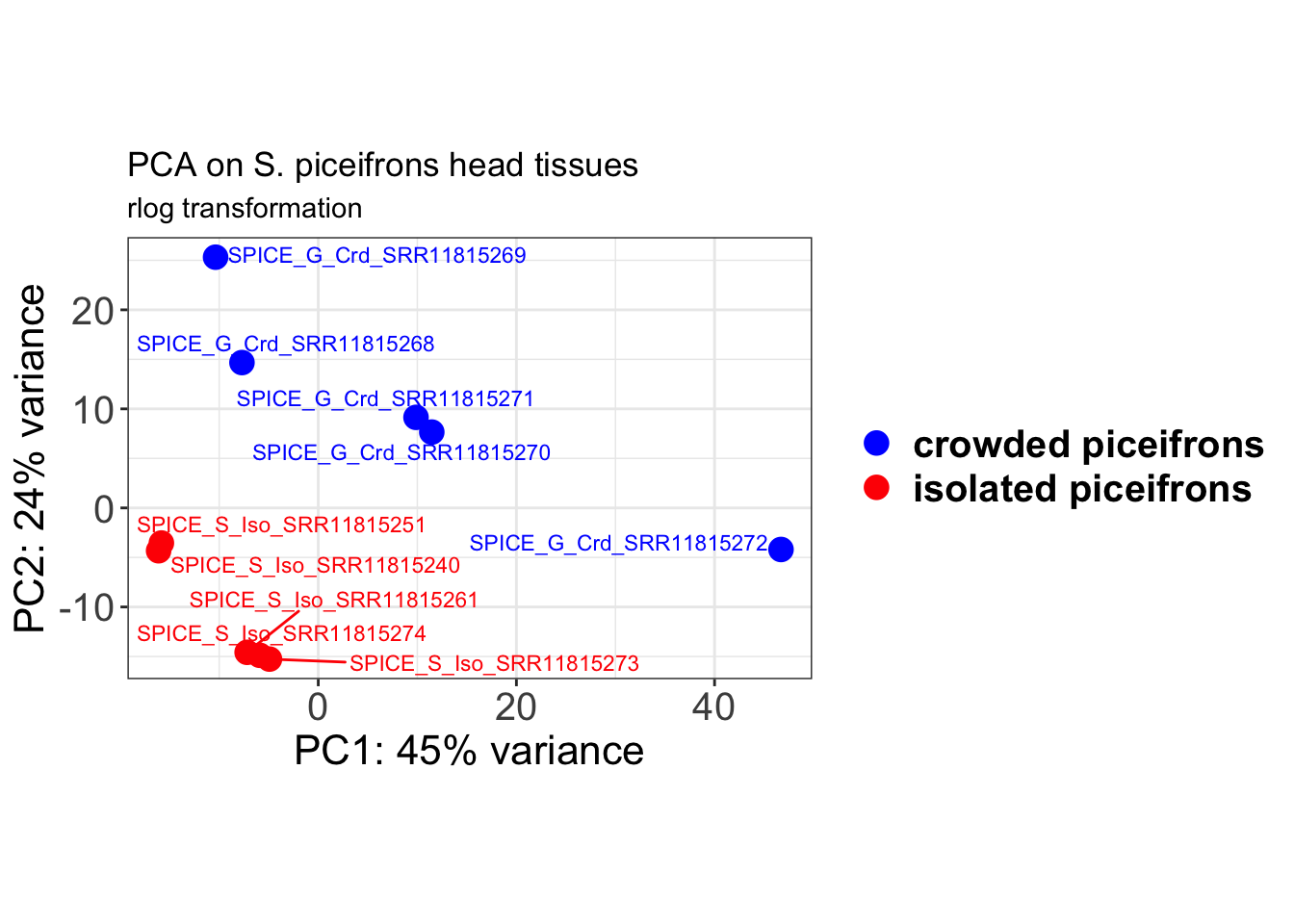
| Version | Author | Date |
|---|---|---|
| 125349f | MaevaTecher | 2022-11-01 |
Plot the PCA vsd
# Create the pca on the defined groups
pcaData <- plotPCA(object = shigeru_vst, intgroup = c("RearingCondition", "Tissue"),
    returnData = TRUE)

# Store the information for each axis variance in %
percentVar <- round(100 * attr(pcaData, "percentVar"))

# Make sure that the discriminant variable are in factor for using shape and
# color later on
pcaData$RearingCondition <- factor(pcaData$RearingCondition, levels = c("Crowded",
    "Isolated"), labels = c("crowded piceifrons", "isolated piceifrons"))
levels(pcaData$RearingCondition)
FALSE [1] "crowded piceifrons" "isolated piceifrons"# pcaData$Tissue<-factor(pcaData1$Tissue,levels=c('Whole_body','Optical_lobes'),
# labels=c('Hatchling', 'OLB')) levels(pcaData$Tissue)
ggplot(pcaData, aes(PC1, PC2, color = RearingCondition)) + geom_point(size = 4) +
xlab(paste0("PC1: ", percentVar[1], "% variance")) + ylab(paste0("PC2: ", percentVar[2],
"% variance")) + scale_color_manual(values = c("blue", "red")) + geom_text_repel(aes(label = name),
nudge_x = -1, nudge_y = 0.2, size = 3) + coord_fixed() + theme_bw() + theme(legend.title = element_blank()) +
theme(legend.text = element_text(face = "bold", size = 15)) + theme(axis.text = element_text(size = 15)) +
theme(axis.title = element_text(size = 16)) + ggtitle("PCA on S. piceifrons head tissues",
subtitle = "vst transformation") + xlab(paste0("PC1: ", percentVar[1], "% variance")) +
ylab(paste0("PC2: ", percentVar[2], "% variance"))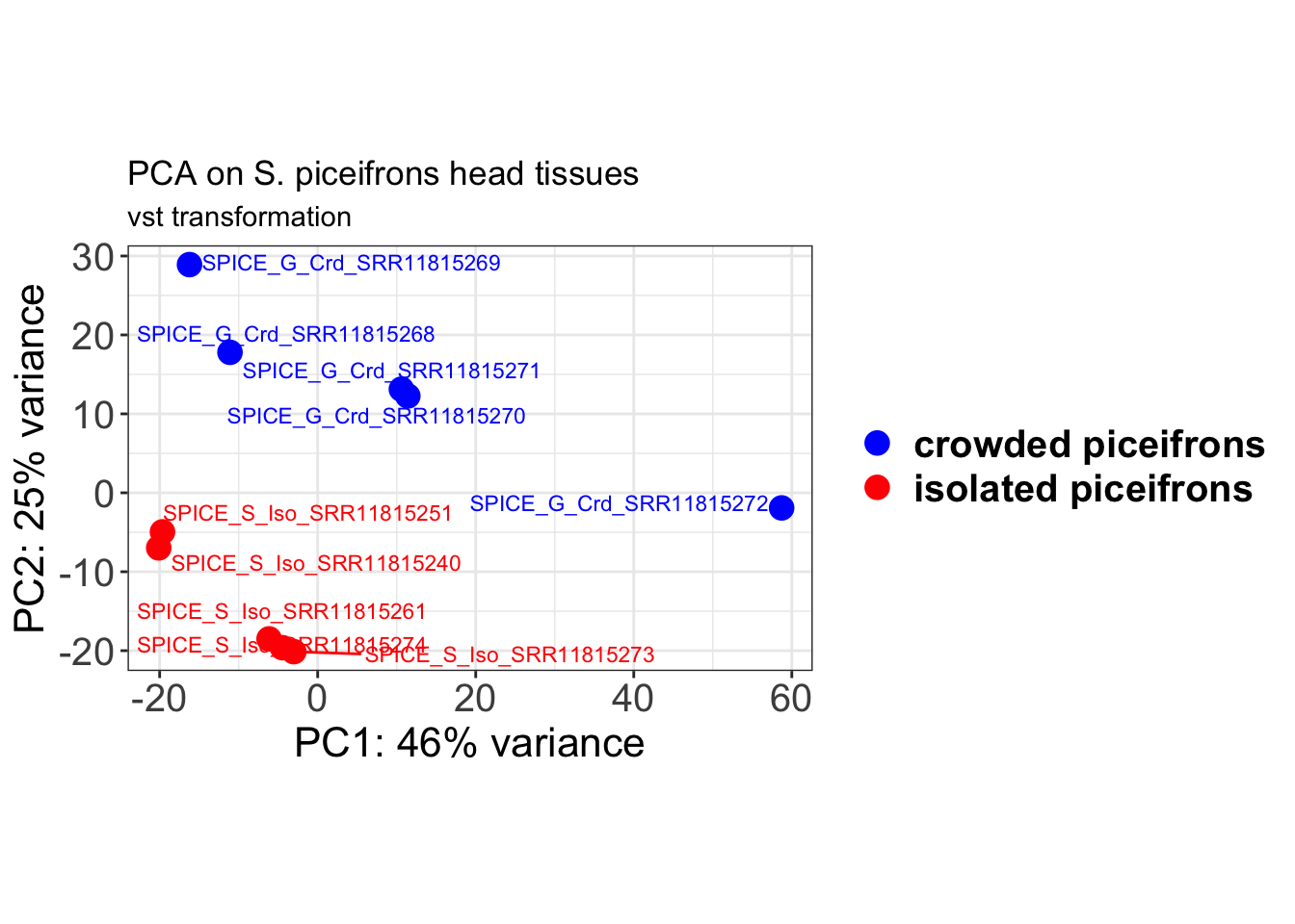
| Version | Author | Date |
|---|---|---|
| 125349f | MaevaTecher | 2022-11-01 |
Sample Matrix Distance
Using also the transformed data, we check the distance between samples and see how they correlate to each others.
Heatmap using rlog
# calculate between-sample distance matrix
sampleDistMatrix.rlog <- as.matrix(dist(t(assay(shigeru_rlog))))

metadata <- sampletable[, c("RearingCondition", "Tissue")]
rownames(metadata) <- sampletable$SampleName


pheatmap(sampleDistMatrix.rlog, annotation_col = metadata, main = "Head tissue heatmap, rlog transformation")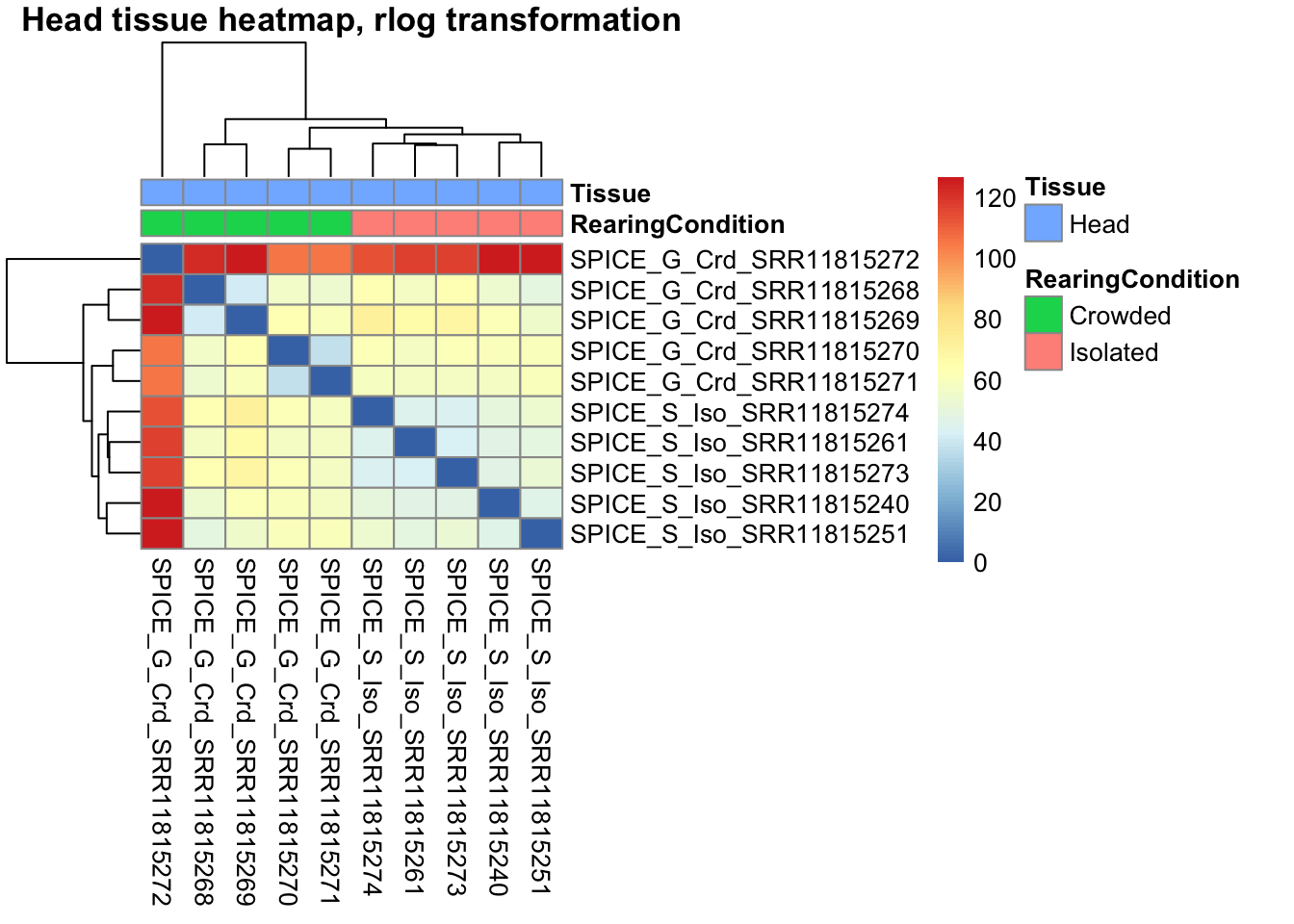
| Version | Author | Date |
|---|---|---|
| 125349f | MaevaTecher | 2022-11-01 |
Heatmap using vst
# calculate between-sample distance matrix
sampleDistMatrix.vst <- as.matrix(dist(t(assay(shigeru_vst))))

pheatmap(sampleDistMatrix.vst, annotation_col = metadata, main = "Head tissue heatmap, vst transformation")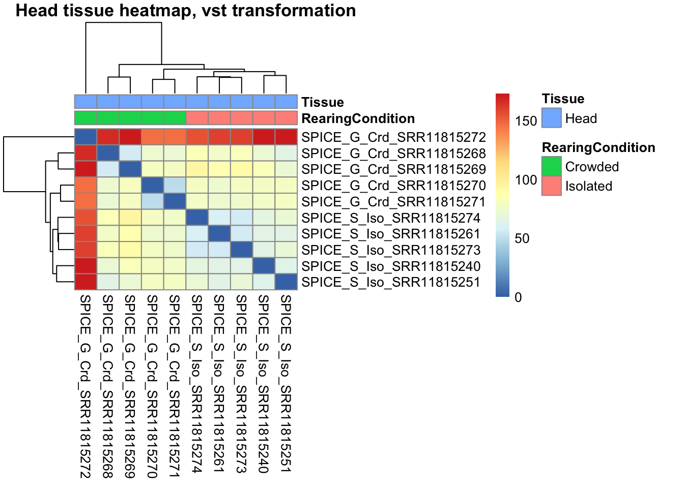
| Version | Author | Date |
|---|---|---|
| 125349f | MaevaTecher | 2022-11-01 |
MA-plot
This plot allows us to show the log2 fold changes over the mean of normalized counts for all the samples. Points will be colored in red if the adjusted p-value is less than 0.05 and the log2 fold change is bigger than 1. In blue, will be the reverse for the log2 fold change.
To generate more accurate log2 foldchange estimates, DESeq2 allows (and recommends) the shrinkage of the LFC estimates toward zero when the information for a gene is low, which could include:
-Low counts
-High dispersion values
# include the log2FoldChange shrinkage use to visualize gene ranking
de_shrink <- lfcShrink(dds = shigeru, coef = "RearingCondition_Isolated_vs_Crowded",
    type = "apeglm")
head(de_shrink)
FALSE log2 fold change (MAP): RearingCondition Isolated vs Crowded
FALSE Wald test p-value: RearingCondition Isolated vs Crowded
FALSE DataFrame with 6 rows and 5 columns
FALSE baseMean log2FoldChange lfcSE pvalue padj
FALSE <numeric> <numeric> <numeric> <numeric> <numeric>
FALSE LOC124796288 2.37306 -0.1187124 0.276337 8.30204e-03 1.12401e-01
FALSE LOC124796294 1.14866 -0.0248082 0.234004 2.80906e-01 NA
FALSE LOC124796332 9.18581 -0.0578750 0.231375 4.01131e-01 7.41676e-01
FALSE LOC124793320 133.76396 -1.1354854 0.865692 4.13290e-03 7.18571e-02
FALSE LOC124712404 29.00252 -0.0797187 0.248051 NA NA
FALSE LOC124798649 11.86003 4.9350149 0.866991 2.46048e-09 6.54487e-07# Ma plot
maplot <- ggmaplot(de_shrink, fdr = 0.05, fc = 1, size = 2, palette = c("#B31B21",
"#1465AC", "darkgray"), genenames = as.vector(rownames(de_shrink$name)), top = 0,
legend = "top", label.select = NULL) + coord_cartesian(xlim = c(0, 20)) + scale_y_continuous(limits = c(-12,
12)) + theme(axis.text.x = element_text(size = 16), axis.text.y = element_text(size = 15),
axis.title.x = element_text(size = 17), axis.title.y = element_text(size = 17),
axis.line = element_line(size = 1, colour = "gray20"), axis.ticks = element_line(size = 1,
colour = "gray20")) + guides(color = guide_legend(override.aes = list(size = c(3,
3, 3)))) + theme(legend.position = c(0.7, 0.12), legend.text = element_text(size = 14,
face = "bold"), legend.background = element_rect(fill = "transparent")) + theme(plot.title = element_text(size = 18,
colour = "gray30", face = "bold", hjust = 0.06, vjust = -5)) + labs(title = "MA-plot for the shrunken log2 fold changes in the head")
maplot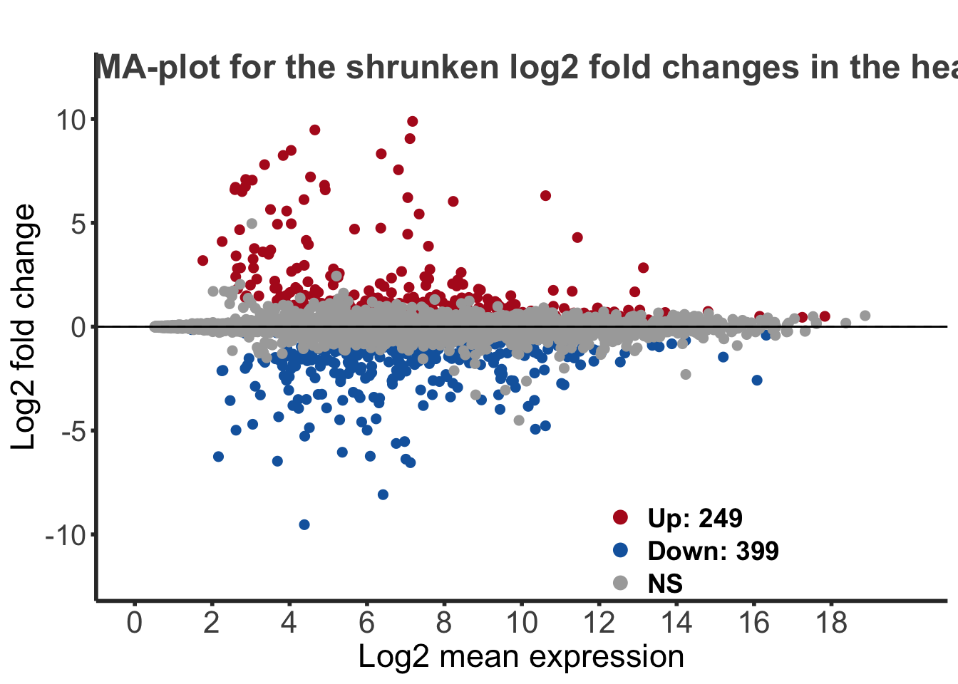
| Version | Author | Date |
|---|---|---|
| 125349f | MaevaTecher | 2022-11-01 |
Volcano Plot
The EnhancedVolcano helps visualise the resulst of
differential expression analysis.
keyvals <- ifelse(res_shigeru$log2FoldChange >= 1 & res_shigeru$padj <= 0.05, "#B31B21",
    ifelse(res_shigeru$log2FoldChange <= -1 & res_shigeru$padj <= 0.05, "#1465AC",
        "darkgray"))

keyvals[is.na(keyvals)] <- "darkgray"
names(keyvals)[keyvals == "#B31B21"] <- "Upregulated"
names(keyvals)[keyvals == "#1465AC"] <- "Downregulated"
names(keyvals)[keyvals == "darkgray"] <- "NS"

EnhancedVolcano(res_shigeru, lab = rownames(res_shigeru), x = "log2FoldChange", y = "padj",
    pCutoff = 0.05, FCcutoff = 1, pointSize = 3, labSize = 4, colAlpha = 4/5, colCustom = keyvals,
    drawConnectors = TRUE)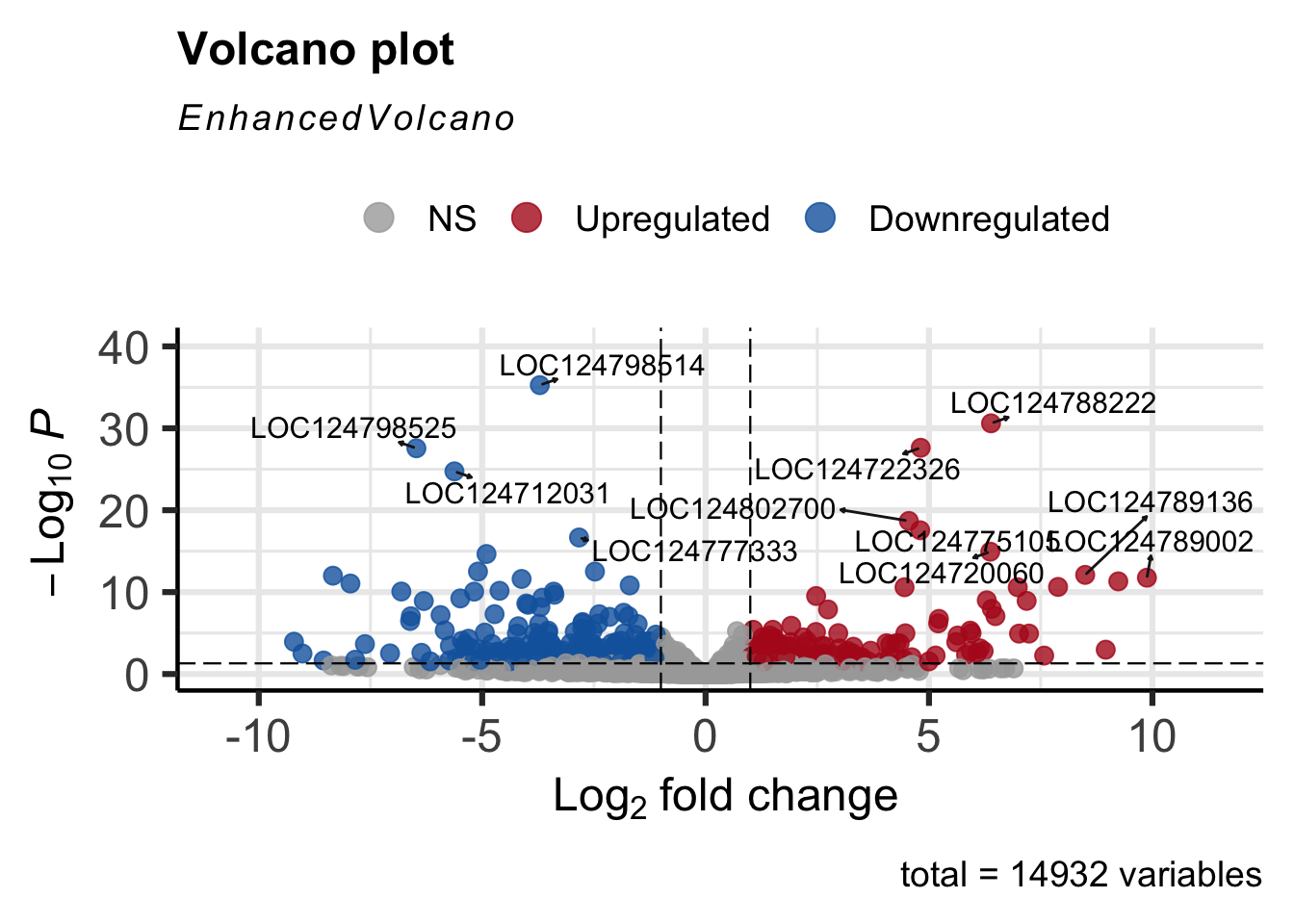
Normalized Matrix distance
We then normalize the result by extracting only significant genes with a fold change of 1.
resorted_deresults <- res_shigeru[order(res_shigeru$padj), ]

## Select only the genes that have a padj > 0.05 and with minimum
## log2FoldChange of 1
sig <- resorted_deresults[!is.na(resorted_deresults$padj) & resorted_deresults$padj <
    tresh_padj & abs(resorted_deresults$log2FoldChange) >= tresh_logfold, ]
selected <- rownames(sig)
selected
FALSE [1] "LOC124798514" "LOC124788222" "LOC124722326" "LOC124798525" "LOC124712031"
FALSE [6] "LOC124802700" "LOC124775105" "LOC124777333" "LOC124720060" "LOC124805215"
FALSE [11] "LOC124804802" "LOC124804688" "LOC124789136" "LOC124804691" "LOC124789002"
FALSE [16] "LOC124804687" "LOC124789650" "LOC124805172" "LOC124791362" "LOC124788242"
FALSE [21] "LOC124777599" "LOC124712054" "LOC124799270" "LOC124789762" "LOC124711568"
FALSE [26] "LOC124805478" "LOC124717267" "LOC124795556" "LOC124789780" "LOC124803056"
FALSE [31] "LOC124802724" "LOC124789001" "LOC124795919" "LOC124802921" "LOC124795391"
FALSE [36] "LOC124802814" "LOC124722943" "LOC124717096" "LOC124798455" "LOC124795472"
FALSE [41] "LOC124718860" "LOC124717260" "LOC124721974" "LOC124800984" "LOC124720306"
FALSE [46] "LOC124791378" "LOC124717148" "LOC124789749" "LOC124798547" "LOC124798649"
FALSE [51] "LOC124777064" "LOC124720432" "LOC124798603" "LOC124798323" "LOC124788214"
FALSE [56] "LOC124789786" "LOC124777258" "LOC124776394" "LOC124777143" "LOC124711857"
FALSE [61] "LOC124787799" "LOC124801935" "LOC124777235" "LOC124803027" "LOC124805241"
FALSE [66] "LOC124718938" "LOC124717283" "LOC124805195" "LOC124799019" "LOC124717389"
FALSE [71] "LOC124720174" "LOC124799061" "LOC124777956" "LOC124795373" "LOC124719983"
FALSE [76] "LOC124712530" "LOC124711778" "LOC124791394" "LOC124721693" "LOC124709245"
FALSE [81] "LOC124718981" "LOC124789632" "LOC124754463" "LOC124719099" "LOC124777576"
FALSE [86] "LOC124721130" "LOC124795430" "LOC124795620" "LOC124803439" "LOC124789548"
FALSE [91] "LOC124712464" "LOC124775601" "LOC124789546" "LOC124796352" "LOC124804686"
FALSE [96] "LOC124789268" "LOC124791708" "LOC124776485" "LOC124720521" "LOC124789741"
FALSE [101] "LOC124805560" "LOC124803748" "LOC124788015" "LOC124803358" "LOC124777671"
FALSE [106] "LOC124797805" "LOC124804656" "LOC124721228" "LOC124795445" "LOC124796321"
FALSE [111] "LOC124777858" "LOC124804813" "LOC124720137" "LOC124795417" "LOC124712047"
FALSE [116] "LOC124712022" "LOC124804598" "LOC124798520" "LOC124710724" "LOC124788290"
FALSE [121] "LOC124797889" "LOC124798208" "LOC124711290" "LOC124795236" "LOC124711697"
FALSE [126] "LOC124711278" "LOC124802776" "LOC124789719" "LOC124711866" "LOC124716714"
FALSE [131] "LOC124776658" "LOC124798509" "LOC124789846" "LOC124712226" "LOC124711548"
FALSE [136] "LOC124798601" "LOC124805162" "LOC124789667" "LOC124719741" "LOC124789397"
FALSE [141] "LOC124777946" "LOC124788119" "LOC124789506" "LOC124795555" "LOC124805313"
FALSE [146] "LOC124805138" "LOC124742380" "LOC124720047" "LOC124716732" "LOC124776026"
FALSE [151] "LOC124802550" "LOC124712519" "LOC124795471" "LOC124795446" "LOC124805178"
FALSE [156] "LOC124787797" "LOC124760025" "LOC124777043" "LOC124712543" "LOC124788266"
FALSE [161] "LOC124711907" "LOC124720355" "LOC124777551" "LOC124795456" "LOC124795184"
FALSE [166] "LOC124794930" "LOC124805680" "LOC124777389" "LOC124789889" "LOC124720076"
FALSE [171] "LOC124711893" "LOC124713151" "LOC124787768" "LOC124790591" "LOC124717061"
FALSE [176] "LOC124722982" "LOC124718923" "LOC124805240" "LOC124773612" "LOC124789965"
FALSE [181] "LOC124802817" "LOC124789336" "LOC124711771" "LOC124719708" "LOC124802707"
FALSE [186] "LOC124777415" "LOC124711951" "LOC124789584" "LOC124719691" "LOC124777491"
FALSE [191] "LOC124789508" "LOC124804665" "LOC124776733" "LOC124711965" "LOC124777770"
FALSE [196] "LOC124776084" "LOC124795141" "LOC124805192" "LOC124798582" "LOC124777662"
FALSE [201] "LOC124798572" "LOC124777899" "LOC124720033" "LOC124776089" "LOC124718862"
FALSE [206] "LOC124805250" "LOC124775969" "LOC124788165" "LOC124742890" "LOC124719815"
FALSE [211] "LOC124797990" "LOC124803348" "LOC124711250" "LOC124775444" "LOC124798698"
FALSE [216] "LOC124799953" "LOC124789795" "LOC124777558" "LOC124803281" "LOC124795918"
FALSE [221] "LOC124711364" "LOC124717265" "LOC124805104" "LOC124777400" "LOC124804991"
FALSE [226] "LOC124794920" "LOC124776202" "LOC124780415" "LOC124794821" "LOC124788012"
FALSE [231] "LOC124776484" "LOC124776648" "LOC124789669" "LOC124719891" "LOC124788914"
FALSE [236] "LOC124802574" "LOC124777923" "LOC124712002" "LOC124777831" "LOC124788538"
FALSE [241] "LOC124787892" "LOC124712552" "LOC124789606" "LOC124798287" "LOC124805339"
FALSE [246] "LOC124777872" "LOC124795640" "LOC124805407" "LOC124718922" "LOC124720476"
FALSE [251] "LOC124722186" "LOC124711793" "LOC124777611" "LOC124722715" "LOC124719969"
FALSE [256] "LOC124798583" "LOC124777594" "LOC124788138" "LOC124722208" "LOC124771028"
FALSE [261] "LOC124790081" "LOC124775415" "LOC124804631" "LOC124719062" "LOC124805532"
FALSE [266] "LOC124787932" "LOC124711752" "LOC124797903" "LOC124711286" "LOC124711861"
FALSE [271] "LOC124789703" "LOC124777762" "LOC124796285" "LOC124789856" "LOC124711994"
FALSE [276] "LOC124777754" "LOC124789687" "LOC124777219" "LOC124776646" "LOC124711943"
FALSE [281] "LOC124777625" "LOC124789886" "LOC124794670" "LOC124777463" "LOC124723001"
FALSE [286] "LOC124804986" "LOC124775213" "LOC124776325" "LOC124776322" "LOC124722471"
FALSE [291] "LOC124777637" "LOC124796310" "LOC124805331" "LOC124717082" "LOC124771313"
FALSE [296] "LOC124776287" "LOC124802884" "LOC124805187" "LOC124800801" "LOC124777187"
FALSE [301] "LOC124718949" "LOC124788080" "LOC124777672" "LOC124776850" "LOC124720168"
FALSE [306] "LOC124722004" "LOC124789575" "LOC124795844" "LOC124799255" "LOC124711859"
FALSE [311] "LOC124711876" "LOC124795649" "LOC124777002" "LOC124720123" "LOC124776707"
FALSE [316] "LOC124796020" "LOC124795457" "LOC124795499" "LOC124789775" "LOC124803230"
FALSE [321] "LOC124802811" "LOC124802970" "LOC124720487" "LOC124716304" "LOC124711910"
FALSE [326] "LOC124776215" "LOC124789613" "LOC124711479" "LOC124795045" "LOC124712049"
FALSE [331] "LOC124779545" "LOC124776760" "LOC124798344" "LOC124794744" "LOC124800634"
FALSE [336] "LOC124798939" "LOC124787813" "LOC124805148" "LOC124795378" "LOC124717171"
FALSE [341] "LOC124805136" "LOC124711197" "LOC124775080" "LOC124795738" "LOC124777512"
FALSE [346] "LOC124795106" "LOC124721091" "LOC124723038" "LOC124803052" "LOC124788368"
FALSE [351] "LOC124777085" "LOC124717333" "LOC124795140" "LOC124795427" "LOC124775853"
FALSE [356] "LOC124796540" "LOC124798392" "LOC124775214" "LOC124717035" "LOC124805664"
FALSE [361] "LOC124795034" "LOC124721604" "LOC124720442" "LOC124796240" "LOC124722978"
FALSE [366] "LOC124789963" "LOC124775408" "LOC124721705" "LOC124722044" "LOC124719056"
FALSE [371] "LOC124738352" "LOC124794714" "LOC124775790" "LOC124777254" "LOC124712021"
FALSE [376] "LOC124787699" "LOC124712088" "LOC124712421" "LOC124717276" "LOC124776630"
FALSE [381] "LOC124788421" "LOC124798325" "LOC124777169" "LOC124789467" "LOC124777204"
FALSE [386] "LOC124718636" "LOC124777722" "LOC124795460" "LOC124789661" "LOC124776010"
FALSE [391] "LOC124711963" "LOC124798334" "LOC124777456" "LOC124717028" "LOC124789869"
FALSE [396] "LOC124723088" "LOC124789858" "LOC124789968" "LOC124711957" "LOC124727296"
FALSE [401] "LOC124718759" "LOC124720170" "LOC124796276" "LOC124775081" "LOC124719067"
FALSE [406] "LOC124798809" "LOC124805413" "LOC124802965" "LOC124716826" "LOC124720038"
FALSE [411] "LOC124711682" "LOC124795954" "LOC124777619" "LOC124777925" "LOC124788526"
FALSE [416] "LOC124711150" "LOC124780975" "LOC124794933" "LOC124720246" "LOC124777364"
FALSE [421] "LOC124770914" "LOC124716906" "LOC124777855" "LOC124777474" "LOC124788385"
FALSE [426] "LOC124788415" "LOC124719754" "LOC124777963" "LOC124789564" "LOC124777771"
FALSE [431] "LOC124776877" "LOC124716851" "LOC124711660" "LOC124777181" "LOC124787635"
FALSE [436] "LOC124795348" "LOC124798671" "LOC124774946" "LOC124717288" "LOC124789692"
FALSE [441] "LOC124802648" "LOC124794839" "LOC124777878" "LOC124788654" "LOC124709336"
FALSE [446] "LOC124798629" "LOC124717160" "LOC124777023" "LOC124791229" "LOC124719813"
FALSE [451] "LOC124780139" "LOC124711754" "LOC124712350" "LOC124803040" "LOC124777097"
FALSE [456] "LOC124798158" "LOC124798250" "LOC124711968" "LOC124790115" "LOC124790046"
FALSE [461] "LOC124776506" "LOC124794873" "LOC124776028" "LOC124777528" "LOC124722901"
FALSE [466] "LOC124805744" "LOC124805010" "LOC124711507" "LOC124711554" "LOC124718598"
FALSE [471] "LOC124777240" "LOC124795583" "LOC124789209" "LOC124802880" "LOC124777757"
FALSE [476] "LOC124789523" "LOC124790095" "LOC124799220" "LOC124787658" "LOC124796406"
FALSE [481] "LOC124711829" "LOC124805064" "LOC124781286" "LOC124722421" "LOC124802832"
FALSE [486] "LOC124709142" "LOC124721844"## Norm transform the data from DEseq2 run
ntd <- normTransform(satoshi)
## Plot the relation among samples considering only the significant genes
pheatmap(assay(ntd)[selected, ], cluster_rows = TRUE, show_rownames = TRUE, cluster_cols = TRUE,
cutree_rows = 4, cutree_cols = 3, labels_col = colData(satoshi)$SampleName)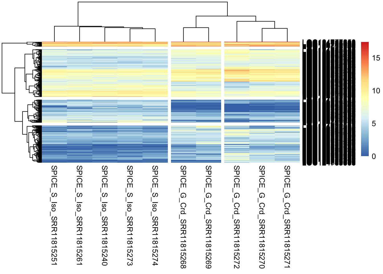
| Version | Author | Date |
|---|---|---|
| 125349f | MaevaTecher | 2022-11-01 |
Create a hmtl report with DEseq2
## import the sample sheet that indicates Rearing Conditions and Tissue origins
setwd(workDir_DEseq2)
# loading target file
target <- loadTargetFile(targetFile = targetFile, varInt = varInt, condRef = condRef,
    batch = batch)
FALSE Target file:
FALSE SampleName
FALSE SPICE_S_Iso_SRR11815240 SPICE_S_Iso_SRR11815240
FALSE SPICE_S_Iso_SRR11815251 SPICE_S_Iso_SRR11815251
FALSE SPICE_S_Iso_SRR11815261 SPICE_S_Iso_SRR11815261
FALSE SPICE_S_Iso_SRR11815273 SPICE_S_Iso_SRR11815273
FALSE SPICE_S_Iso_SRR11815274 SPICE_S_Iso_SRR11815274
FALSE SPICE_G_Crd_SRR11815268 SPICE_G_Crd_SRR11815268
FALSE SPICE_G_Crd_SRR11815269 SPICE_G_Crd_SRR11815269
FALSE SPICE_G_Crd_SRR11815270 SPICE_G_Crd_SRR11815270
FALSE SPICE_G_Crd_SRR11815271 SPICE_G_Crd_SRR11815271
FALSE SPICE_G_Crd_SRR11815272 SPICE_G_Crd_SRR11815272
FALSE FileName Tissue
FALSE SPICE_S_Iso_SRR11815240 SPICE_S_Iso_SRR11815240_counts.txt Head
FALSE SPICE_S_Iso_SRR11815251 SPICE_S_Iso_SRR11815251_counts.txt Head
FALSE SPICE_S_Iso_SRR11815261 SPICE_S_Iso_SRR11815261_counts.txt Head
FALSE SPICE_S_Iso_SRR11815273 SPICE_S_Iso_SRR11815273_counts.txt Head
FALSE SPICE_S_Iso_SRR11815274 SPICE_S_Iso_SRR11815274_counts.txt Head
FALSE SPICE_G_Crd_SRR11815268 SPICE_G_Crd_SRR11815268_counts.txt Head
FALSE SPICE_G_Crd_SRR11815269 SPICE_G_Crd_SRR11815269_counts.txt Head
FALSE SPICE_G_Crd_SRR11815270 SPICE_G_Crd_SRR11815270_counts.txt Head
FALSE SPICE_G_Crd_SRR11815271 SPICE_G_Crd_SRR11815271_counts.txt Head
FALSE SPICE_G_Crd_SRR11815272 SPICE_G_Crd_SRR11815272_counts.txt Head
FALSE RearingCondition
FALSE SPICE_S_Iso_SRR11815240 Isolated
FALSE SPICE_S_Iso_SRR11815251 Isolated
FALSE SPICE_S_Iso_SRR11815261 Isolated
FALSE SPICE_S_Iso_SRR11815273 Isolated
FALSE SPICE_S_Iso_SRR11815274 Isolated
FALSE SPICE_G_Crd_SRR11815268 Crowded
FALSE SPICE_G_Crd_SRR11815269 Crowded
FALSE SPICE_G_Crd_SRR11815270 Crowded
FALSE SPICE_G_Crd_SRR11815271 Crowded
FALSE SPICE_G_Crd_SRR11815272 Crowded# loading counts
counts <- loadCountData(target = target, rawDir = rawDir, featuresToRemove = featuresToRemove)FALSE Loading files:
FALSE SPICE_S_Iso_SRR11815240_counts.txt: 28731 rows and 14531 null count(s)
FALSE SPICE_S_Iso_SRR11815251_counts.txt: 28731 rows and 14513 null count(s)
FALSE SPICE_S_Iso_SRR11815261_counts.txt: 28731 rows and 14392 null count(s)
FALSE SPICE_S_Iso_SRR11815273_counts.txt: 28731 rows and 14221 null count(s)
FALSE SPICE_S_Iso_SRR11815274_counts.txt: 28731 rows and 14424 null count(s)
FALSE SPICE_G_Crd_SRR11815268_counts.txt: 28731 rows and 14657 null count(s)
FALSE SPICE_G_Crd_SRR11815269_counts.txt: 28731 rows and 14521 null count(s)
FALSE SPICE_G_Crd_SRR11815270_counts.txt: 28731 rows and 14504 null count(s)
FALSE SPICE_G_Crd_SRR11815271_counts.txt: 28731 rows and 14059 null count(s)
FALSE SPICE_G_Crd_SRR11815272_counts.txt: 28731 rows and 15232 null count(s)
FALSE
FALSE Features removed:
FALSE
FALSE Top of the counts matrix:
FALSE SPICE_S_Iso_SRR11815240 SPICE_S_Iso_SRR11815251
FALSE LOC124708997 610 562
FALSE LOC124708998 510 407
FALSE LOC124708999 0 1
FALSE LOC124709000 2 0
FALSE LOC124709001 0 0
FALSE LOC124709003 0 0
FALSE SPICE_S_Iso_SRR11815261 SPICE_S_Iso_SRR11815273
FALSE LOC124708997 3346 8876
FALSE LOC124708998 891 692
FALSE LOC124708999 0 0
FALSE LOC124709000 2 4
FALSE LOC124709001 0 0
FALSE LOC124709003 0 0
FALSE SPICE_S_Iso_SRR11815274 SPICE_G_Crd_SRR11815268
FALSE LOC124708997 4341 343
FALSE LOC124708998 773 439
FALSE LOC124708999 0 0
FALSE LOC124709000 4 2
FALSE LOC124709001 1 0
FALSE LOC124709003 0 0
FALSE SPICE_G_Crd_SRR11815269 SPICE_G_Crd_SRR11815270
FALSE LOC124708997 314 463
FALSE LOC124708998 461 799
FALSE LOC124708999 0 0
FALSE LOC124709000 0 0
FALSE LOC124709001 0 0
FALSE LOC124709003 0 2
FALSE SPICE_G_Crd_SRR11815271 SPICE_G_Crd_SRR11815272
FALSE LOC124708997 638 3170
FALSE LOC124708998 936 496
FALSE LOC124708999 0 0
FALSE LOC124709000 0 0
FALSE LOC124709001 0 0
FALSE LOC124709003 0 0
FALSE
FALSE Bottom of the counts matrix:
FALSE SPICE_S_Iso_SRR11815240 SPICE_S_Iso_SRR11815251
FALSE Trnav-cac 0 0
FALSE Trnav-gac 0 0
FALSE Trnav-uac 0 0
FALSE Trnaw-cca 0 0
FALSE Trnay-aua 0 0
FALSE Trnay-gua 0 0
FALSE SPICE_S_Iso_SRR11815261 SPICE_S_Iso_SRR11815273
FALSE Trnav-cac 0 0
FALSE Trnav-gac 0 0
FALSE Trnav-uac 0 0
FALSE Trnaw-cca 0 0
FALSE Trnay-aua 0 0
FALSE Trnay-gua 0 0
FALSE SPICE_S_Iso_SRR11815274 SPICE_G_Crd_SRR11815268
FALSE Trnav-cac 0 0
FALSE Trnav-gac 0 0
FALSE Trnav-uac 0 0
FALSE Trnaw-cca 0 0
FALSE Trnay-aua 0 0
FALSE Trnay-gua 0 0
FALSE SPICE_G_Crd_SRR11815269 SPICE_G_Crd_SRR11815270
FALSE Trnav-cac 0 0
FALSE Trnav-gac 0 0
FALSE Trnav-uac 0 0
FALSE Trnaw-cca 0 0
FALSE Trnay-aua 0 0
FALSE Trnay-gua 0 0
FALSE SPICE_G_Crd_SRR11815271 SPICE_G_Crd_SRR11815272
FALSE Trnav-cac 0 0
FALSE Trnav-gac 0 0
FALSE Trnav-uac 0 0
FALSE Trnaw-cca 0 0
FALSE Trnay-aua 0 0
FALSE Trnay-gua 0 0# description plots
majSequences <- descriptionPlots(counts = counts, group = target[, varInt], col = colors)FALSE Matrix of SERE statistics:
FALSE SPICE_S_Iso_SRR11815240 SPICE_S_Iso_SRR11815251
FALSE SPICE_S_Iso_SRR11815240 0.000 7.681
FALSE SPICE_S_Iso_SRR11815251 7.681 0.000
FALSE SPICE_S_Iso_SRR11815261 8.278 7.525
FALSE SPICE_S_Iso_SRR11815273 8.073 8.239
FALSE SPICE_S_Iso_SRR11815274 7.342 8.961
FALSE SPICE_G_Crd_SRR11815268 8.750 5.271
FALSE SPICE_G_Crd_SRR11815269 10.462 6.957
FALSE SPICE_G_Crd_SRR11815270 11.375 8.585
FALSE SPICE_G_Crd_SRR11815271 10.225 7.865
FALSE SPICE_G_Crd_SRR11815272 21.111 20.214
FALSE SPICE_S_Iso_SRR11815261 SPICE_S_Iso_SRR11815273
FALSE SPICE_S_Iso_SRR11815240 8.278 8.073
FALSE SPICE_S_Iso_SRR11815251 7.525 8.239
FALSE SPICE_S_Iso_SRR11815261 0.000 6.150
FALSE SPICE_S_Iso_SRR11815273 6.150 0.000
FALSE SPICE_S_Iso_SRR11815274 7.051 6.487
FALSE SPICE_G_Crd_SRR11815268 8.817 9.755
FALSE SPICE_G_Crd_SRR11815269 11.514 11.846
FALSE SPICE_G_Crd_SRR11815270 11.274 11.696
FALSE SPICE_G_Crd_SRR11815271 9.681 10.195
FALSE SPICE_G_Crd_SRR11815272 21.701 21.430
FALSE SPICE_S_Iso_SRR11815274 SPICE_G_Crd_SRR11815268
FALSE SPICE_S_Iso_SRR11815240 7.342 8.750
FALSE SPICE_S_Iso_SRR11815251 8.961 5.271
FALSE SPICE_S_Iso_SRR11815261 7.051 8.817
FALSE SPICE_S_Iso_SRR11815273 6.487 9.755
FALSE SPICE_S_Iso_SRR11815274 0.000 10.433
FALSE SPICE_G_Crd_SRR11815268 10.433 0.000
FALSE SPICE_G_Crd_SRR11815269 12.567 5.995
FALSE SPICE_G_Crd_SRR11815270 12.590 6.881
FALSE SPICE_G_Crd_SRR11815271 10.910 7.054
FALSE SPICE_G_Crd_SRR11815272 20.887 19.749
FALSE SPICE_G_Crd_SRR11815269 SPICE_G_Crd_SRR11815270
FALSE SPICE_S_Iso_SRR11815240 10.462 11.375
FALSE SPICE_S_Iso_SRR11815251 6.957 8.585
FALSE SPICE_S_Iso_SRR11815261 11.514 11.274
FALSE SPICE_S_Iso_SRR11815273 11.846 11.696
FALSE SPICE_S_Iso_SRR11815274 12.567 12.590
FALSE SPICE_G_Crd_SRR11815268 5.995 6.881
FALSE SPICE_G_Crd_SRR11815269 0.000 8.480
FALSE SPICE_G_Crd_SRR11815270 8.480 0.000
FALSE SPICE_G_Crd_SRR11815271 8.659 6.828
FALSE SPICE_G_Crd_SRR11815272 20.361 20.568
FALSE SPICE_G_Crd_SRR11815271 SPICE_G_Crd_SRR11815272
FALSE SPICE_S_Iso_SRR11815240 10.225 21.111
FALSE SPICE_S_Iso_SRR11815251 7.865 20.214
FALSE SPICE_S_Iso_SRR11815261 9.681 21.701
FALSE SPICE_S_Iso_SRR11815273 10.195 21.430
FALSE SPICE_S_Iso_SRR11815274 10.910 20.887
FALSE SPICE_G_Crd_SRR11815268 7.054 19.749
FALSE SPICE_G_Crd_SRR11815269 8.659 20.361
FALSE SPICE_G_Crd_SRR11815270 6.828 20.568
FALSE SPICE_G_Crd_SRR11815271 0.000 20.397
FALSE SPICE_G_Crd_SRR11815272 20.397 0.000# analysis with DESeq2
out.DESeq2 <- run.DESeq2(counts = counts, target = target, varInt = varInt, batch = batch,
locfunc = locfunc, fitType = fitType, pAdjustMethod = pAdjustMethod_DEseq2, cooksCutoff = cooksCutoff,
independentFiltering = independentFiltering, alpha = alpha_DEseq2)FALSE Design of the statistical model:
FALSE ~ RearingCondition
FALSE
FALSE Normalization factors:
FALSE SPICE_S_Iso_SRR11815240 SPICE_S_Iso_SRR11815251 SPICE_S_Iso_SRR11815261
FALSE 0.9298497 0.9129101 1.4552040
FALSE SPICE_S_Iso_SRR11815273 SPICE_S_Iso_SRR11815274 SPICE_G_Crd_SRR11815268
FALSE 1.3328683 1.1726994 0.8242531
FALSE SPICE_G_Crd_SRR11815269 SPICE_G_Crd_SRR11815270 SPICE_G_Crd_SRR11815271
FALSE 0.9639351 1.1943765 1.3987534
FALSE SPICE_G_Crd_SRR11815272
FALSE 0.4421667
FALSE Comparison Crowded vs Isolated done# PCA + Clustering
exploreCounts(object = out.DESeq2$dds, group = target[, varInt], typeTrans = typeTrans,
col = colors)FALSE quartz_off_screen
FALSE 2# summary of the analysis (boxplots, dispersions, diag size factors, export
# table, nDiffTotal, histograms, MA plot)
summaryResults <- summarizeResults.DESeq2(out.DESeq2, group = target[, varInt], col = colors,
independentFiltering = independentFiltering, cooksCutoff = cooksCutoff, alpha = alpha_DEseq2)FALSE Number of features discarded by the independent filtering:
FALSE Test vs Ref BaseMean Threshold # discarded
FALSE [1,] Crowded vs Isolated 1.79 14994
FALSE
FALSE Number of features down/up and total:
FALSE Test vs Ref # down # up # total
FALSE [1,] Crowded vs Isolated 248 394 642# generating HTML report
writeReport.DESeq2(target = target, counts = counts, out.DESeq2 = out.DESeq2, summaryResults = summaryResults,
majSequences = majSequences, workDir = workDir_DEseq2, projectName = projectName,
author = author, targetFile = targetFile, rawDir = rawDir, featuresToRemove = featuresToRemove,
varInt = varInt, condRef = condRef, batch = batch, fitType = fitType, cooksCutoff = cooksCutoff,
independentFiltering = independentFiltering, alpha = alpha_DEseq2, pAdjustMethod = pAdjustMethod_DEseq2,
typeTrans = typeTrans, locfunc = locfunc, colors = colors)FALSE HTML report created
sessionInfo()FALSE R version 4.2.1 (2022-06-23)
FALSE Platform: x86_64-apple-darwin17.0 (64-bit)
FALSE Running under: macOS Big Sur ... 10.16
FALSE
FALSE Matrix products: default
FALSE BLAS: /Library/Frameworks/R.framework/Versions/4.2/Resources/lib/libRblas.0.dylib
FALSE LAPACK: /Library/Frameworks/R.framework/Versions/4.2/Resources/lib/libRlapack.dylib
FALSE
FALSE locale:
FALSE [1] en_US.UTF-8/en_US.UTF-8/en_US.UTF-8/C/en_US.UTF-8/en_US.UTF-8
FALSE
FALSE attached base packages:
FALSE [1] stats4 stats graphics grDevices utils datasets methods
FALSE [8] base
FALSE
FALSE other attached packages:
FALSE [1] pheatmap_1.0.12 SARTools_1.8.1
FALSE [3] kableExtra_1.3.4 edgeR_3.38.4
FALSE [5] limma_3.52.4 ashr_2.2-54
FALSE [7] EnhancedVolcano_1.14.0 ggrepel_0.9.1
FALSE [9] ggpubr_0.4.0 apeglm_1.18.0
FALSE [11] data.table_1.14.4 DESeq2_1.36.0
FALSE [13] SummarizedExperiment_1.26.1 Biobase_2.56.0
FALSE [15] MatrixGenerics_1.8.1 matrixStats_0.62.0
FALSE [17] GenomicRanges_1.48.0 GenomeInfoDb_1.32.4
FALSE [19] IRanges_2.31.2 S4Vectors_0.34.0
FALSE [21] BiocGenerics_0.42.0 reshape2_1.4.4
FALSE [23] ggthemes_4.2.4 plotly_4.10.0
FALSE [25] DT_0.26 forcats_0.5.2
FALSE [27] stringr_1.4.1 dplyr_1.0.10
FALSE [29] purrr_0.3.5 readr_2.1.3
FALSE [31] tidyr_1.2.1 tibble_3.1.8
FALSE [33] ggplot2_3.3.6 tidyverse_1.3.2
FALSE [35] rmdformats_1.0.4 knitr_1.40
FALSE
FALSE loaded via a namespace (and not attached):
FALSE [1] readxl_1.4.1 backports_1.4.1 workflowr_1.7.0
FALSE [4] systemfonts_1.0.4 plyr_1.8.7 lazyeval_0.2.2
FALSE [7] splines_4.2.1 BiocParallel_1.30.4 digest_0.6.30
FALSE [10] invgamma_1.1 htmltools_0.5.3 SQUAREM_2021.1
FALSE [13] fansi_1.0.3 magrittr_2.0.3 memoise_2.0.1
FALSE [16] googlesheets4_1.0.1 tzdb_0.3.0 Biostrings_2.64.1
FALSE [19] annotate_1.74.0 modelr_0.1.9 svglite_2.1.0
FALSE [22] bdsmatrix_1.3-6 colorspace_2.0-3 blob_1.2.3
FALSE [25] rvest_1.0.3 haven_2.5.1 xfun_0.34
FALSE [28] crayon_1.5.2 RCurl_1.98-1.9 jsonlite_1.8.3
FALSE [31] genefilter_1.78.0 survival_3.4-0 glue_1.6.2
FALSE [34] gtable_0.3.1 gargle_1.2.1 zlibbioc_1.42.0
FALSE [37] XVector_0.36.0 webshot_0.5.4 DelayedArray_0.22.0
FALSE [40] car_3.1-1 abind_1.4-5 scales_1.2.1
FALSE [43] mvtnorm_1.1-3 GGally_2.1.2 DBI_1.1.3
FALSE [46] rstatix_0.7.0 Rcpp_1.0.9 viridisLite_0.4.1
FALSE [49] xtable_1.8-4 emdbook_1.3.12 bit_4.0.4
FALSE [52] truncnorm_1.0-8 htmlwidgets_1.5.4 httr_1.4.4
FALSE [55] RColorBrewer_1.1-3 ellipsis_0.3.2 farver_2.1.1
FALSE [58] reshape_0.8.9 pkgconfig_2.0.3 XML_3.99-0.11
FALSE [61] sass_0.4.2 dbplyr_2.2.1 locfit_1.5-9.6
FALSE [64] utf8_1.2.2 labeling_0.4.2 tidyselect_1.2.0
FALSE [67] rlang_1.0.6 later_1.3.0 AnnotationDbi_1.58.0
FALSE [70] munsell_0.5.0 cellranger_1.1.0 tools_4.2.1
FALSE [73] cachem_1.0.6 cli_3.4.1 generics_0.1.3
FALSE [76] RSQLite_2.2.18 broom_1.0.1 ggdendro_0.1.23
FALSE [79] evaluate_0.17 fastmap_1.1.0 yaml_2.3.6
FALSE [82] bit64_4.0.5 fs_1.5.2 KEGGREST_1.36.3
FALSE [85] whisker_0.4 formatR_1.12 xml2_1.3.3
FALSE [88] compiler_4.2.1 rstudioapi_0.14 png_0.1-7
FALSE [91] ggsignif_0.6.4 reprex_2.0.2 geneplotter_1.74.0
FALSE [94] bslib_0.4.0 stringi_1.7.8 highr_0.9
FALSE [97] lattice_0.20-45 Matrix_1.5-1 vctrs_0.5.0
FALSE [100] pillar_1.8.1 lifecycle_1.0.3 jquerylib_0.1.4
FALSE [103] irlba_2.3.5.1 bitops_1.0-7 httpuv_1.6.6
FALSE [106] R6_2.5.1 bookdown_0.29 promises_1.2.0.1
FALSE [109] gridExtra_2.3 codetools_0.2-18 MASS_7.3-58.1
FALSE [112] assertthat_0.2.1 rprojroot_2.0.3 withr_2.5.0
FALSE [115] GenomeInfoDbData_1.2.8 parallel_4.2.1 hms_1.1.2
FALSE [118] grid_4.2.1 coda_0.19-4 rmarkdown_2.17
FALSE [121] carData_3.0-5 googledrive_2.0.0 git2r_0.30.1
FALSE [124] mixsqp_0.3-43 bbmle_1.0.25 numDeriv_2016.8-1.1
FALSE [127] lubridate_1.8.0