Last updated: 2024-10-11

Checks: 7 0

Knit directory: mito_age_fert/

This reproducible R Markdown analysis was created with workflowr (version 1.7.1). The Checks tab describes the reproducibility checks that were applied when the results were created. The Past versions tab lists the development history.

R Markdown file: up-to-date

Great! Since the R Markdown file has been committed to the Git repository, you know the exact version of the code that produced these results.

Environment: empty

Great job! The global environment was empty. Objects defined in the global environment can affect the analysis in your R Markdown file in unknown ways. For reproduciblity it’s best to always run the code in an empty environment.

Seed: set.seed(20230213)

The command set.seed(20230213) was run prior to running the code in the R Markdown file. Setting a seed ensures that any results that rely on randomness, e.g. subsampling or permutations, are reproducible.

Session information: recorded

Great job! Recording the operating system, R version, and package versions is critical for reproducibility.

Cache: none

Nice! There were no cached chunks for this analysis, so you can be confident that you successfully produced the results during this run.

File paths: relative

Great job! Using relative paths to the files within your workflowr project makes it easier to run your code on other machines.

Repository version: 0f5ea81

Great! You are using Git for version control. Tracking code development and connecting the code version to the results is critical for reproducibility.

The results in this page were generated with repository version 0f5ea81. See the Past versions tab to see a history of the changes made to the R Markdown and HTML files.

Note that you need to be careful to ensure that all relevant files for the analysis have been committed to Git prior to generating the results (you can use wflow_publish or wflow_git_commit). workflowr only checks the R Markdown file, but you know if there are other scripts or data files that it depends on. Below is the status of the Git repository when the results were generated:


Ignored files:
    Ignored:    .DS_Store
    Ignored:    .Rhistory
    Ignored:    .Rproj.user/
    Ignored:    analysis/.DS_Store
    Ignored:    analysis/figure/
    Ignored:    data/.DS_Store

Untracked files:
    Untracked:  README.html
    Untracked:  check_lines.R
    Untracked:  code/data_wrangling.R
    Untracked:  code/plotting_Script.R
    Untracked:  data/Data_raw_emmely.csv
    Untracked:  data/defence.csv
    Untracked:  data/male_fertility.csv
    Untracked:  data/mito_34sigdiffSNPs_consensus_incl_colnames.csv
    Untracked:  data/mito_mt_copy_number.xlsx
    Untracked:  data/mito_mt_seq_major_alleles_sig_snptable.csv
    Untracked:  data/mito_mt_seq_sig_annotated.csv
    Untracked:  data/mito_mt_seq_sig_annotated.vcf
    Untracked:  data/offence.csv
    Untracked:  data/rawdata_PCA.csv
    Untracked:  data/snp-gene.txt
    Untracked:  data/sperm_metabolic_rate.csv
    Untracked:  data/sperm_viability.csv
    Untracked:  data/wrangled/
    Untracked:  figures/
    Untracked:  output/SNP_clusters.csv
    Untracked:  output/bod_brm.rds
    Untracked:  output/female_rate_dredge.rds
    Untracked:  output/female_rates_bb.Rdata
    Untracked:  output/female_rates_boot.Rdata
    Untracked:  output/female_rates_poly.Rdata
    Untracked:  output/male_fec_dredge.rds
    Untracked:  output/male_hatch_dredge.rds
    Untracked:  output/male_hatch_dredge_reduced.rds
    Untracked:  output/sperm_met_dredge.rds
    Untracked:  output/viab_ctrl_dredge.rds
    Untracked:  output/viab_trt_dredge.rds
    Untracked:  snp_matrix_dobler.csv

Unstaged changes:
    Deleted:    analysis/sperm_comp.Rmd
    Modified:   data/README.md

Note that any generated files, e.g. HTML, png, CSS, etc., are not included in this status report because it is ok for generated content to have uncommitted changes.

These are the previous versions of the repository in which changes were made to the R Markdown (analysis/female_fertility.Rmd) and HTML (docs/female_fertility.html) files. If you’ve configured a remote Git repository (see ?wflow_git_remote), click on the hyperlinks in the table below to view the files as they were in that past version.

File	Version	Author	Date	Message
Rmd	0f5ea81	MartinGarlovsky	2024-10-11	wflow_publish("analysis/female_fertility.Rmd")
html	2ee8510	MartinGarlovsky	2024-10-09	Build site.
Rmd	2eea37b	MartinGarlovsky	2024-10-09	wflow_publish("analysis/female_fertility.Rmd")

Load packages

library(tidyverse)

library(lme4)
#library(merTools)
library(DHARMa)
library(emmeans)
library(kableExtra)
library(knitrhooks) # install with devtools::install_github("nathaneastwood/knitrhooks")
library(showtext)

library(conflicted)

select <- dplyr::select
filter <- dplyr::filter

output_max_height() # a knitrhook option

options(stringsAsFactors = FALSE)

# colour palettes
met.pal <- MetBrewer::met.brewer('Johnson')
met3 <- met.pal[c(1, 3, 5)]

# set contrasts
options(contrasts = c("contr.sum", "contr.poly"))

Load data

fert_dat <- read_csv("data/wrangled/female_fertility.csv") %>% 
  mutate(mito_snp = as.factor(mito_snp),
         coevolved = if_else(mito == nuclear, "matched", "mismatched"))

Introduction

First look at the data shows that fecundity appears to plateau between the first and second vial before declining. Therefore, we model fecundity across three episodes:

early life fecundity
lifetime fecundity
the rate of progeny production

# progeny by mito / nuclear
fert_dat %>% 
  group_by(mito, nuclear, vial) %>% 
  summarise(mn = mean(progeny),
            se = sd(progeny)/sqrt(n()),
            s95 = se * 1.96) %>% 
  ggplot(aes(x = vial, y = mn, colour = mito)) +
  geom_point(data = fert_dat,
             aes(y = progeny, colour = mito), alpha = .15,
             position = position_jitterdodge(dodge.width = .5, jitter.width = .1)) +
  geom_ribbon(aes(ymin = mn - s95, ymax = mn + s95, fill = mito, group = mito),
              alpha = .5, colour = NA) +
  geom_errorbar(aes(ymin = mn - s95, ymax = mn + s95), 
                width = .25, position = position_dodge(width = .5)) +
  geom_point(position = position_dodge(width = .5)) +
  geom_line(aes(group = nuclear)) + 
  facet_wrap(~nuclear) +
  scale_x_continuous(breaks = c(1:7)) +
  scale_colour_manual(values = met3) +
  scale_fill_manual(values = met3) +
  labs(y = 'Fecundity per vial (EMM ± 95% CIs)') +
  theme_bw() + 
  theme() + 
  #ggsave('figures/vial_means.pdf', height = 3, width = 9, dpi = 600, useDingbats = FALSE) +
  NULL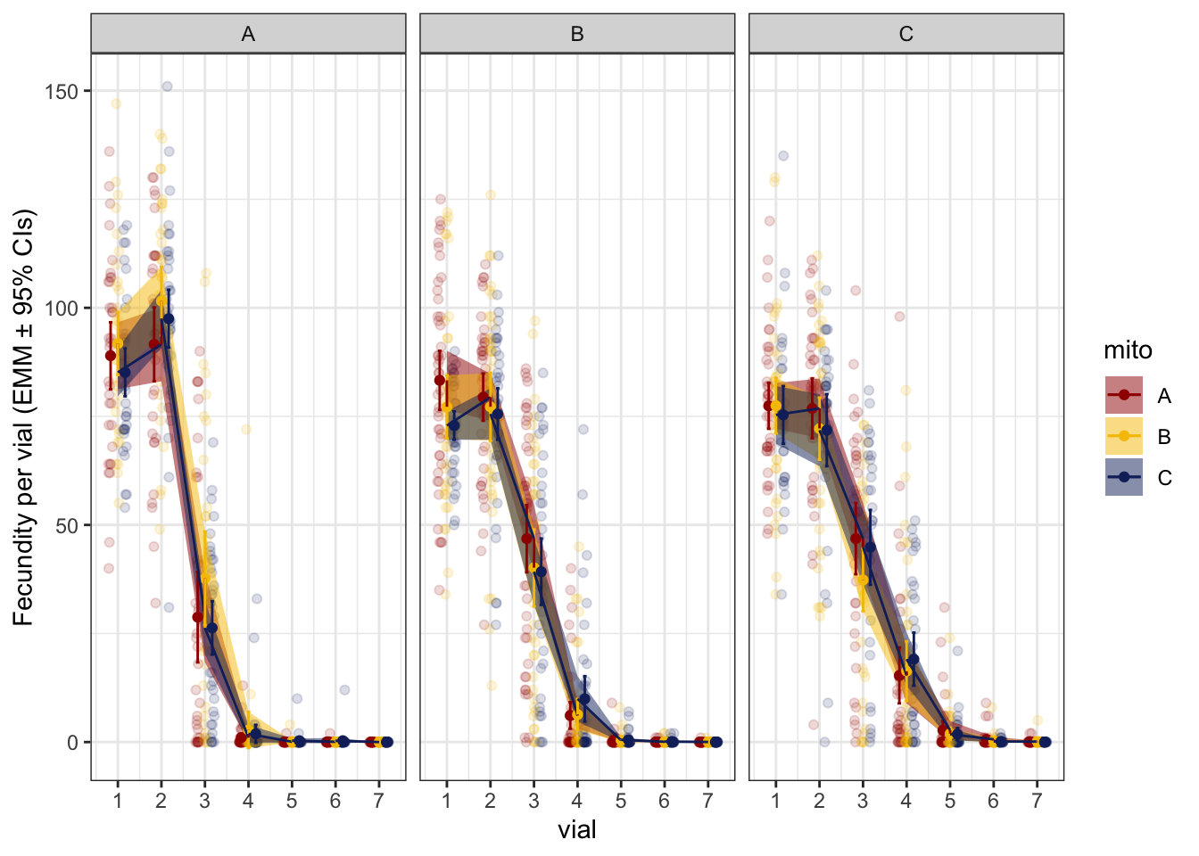

Version	Author	Date
2ee8510	MartinGarlovsky	2024-10-09

Figure 1. Per vial progeny production for each mitonculear genotype. Facets are nuclear genotypes, with colour denoting mitochondrial genotype.

> Early life fecundity

We summed progeny produced from the first two vial for each female.

daydat <- fert_dat %>% filter(vial == '1' | vial == '2') %>% 
  dplyr::select(ID:mtn, mito_snp, coevolved, LINE, vial, progeny) %>% 
  pivot_wider(names_from = vial,
              values_from = progeny) %>% 
  dplyr::rename(v1 = `1`, v2 = `2`) %>% 
  mutate(comb_vial = rowSums(across(c(v1, v2))))

daydat %>% pivot_longer(cols = c(v1, v2)) %>% #filter(age == "young") %>% 
  ggplot(aes(x = name, y = value)) + 
  geom_line(aes(group = ID, colour = mito)) +
  tidybayes::stat_halfeye(alpha = .5) +
  scale_colour_manual(values = met3) +
  labs(y = 'Female fecundity') +
  facet_grid(mito ~ nuclear) +
  NULL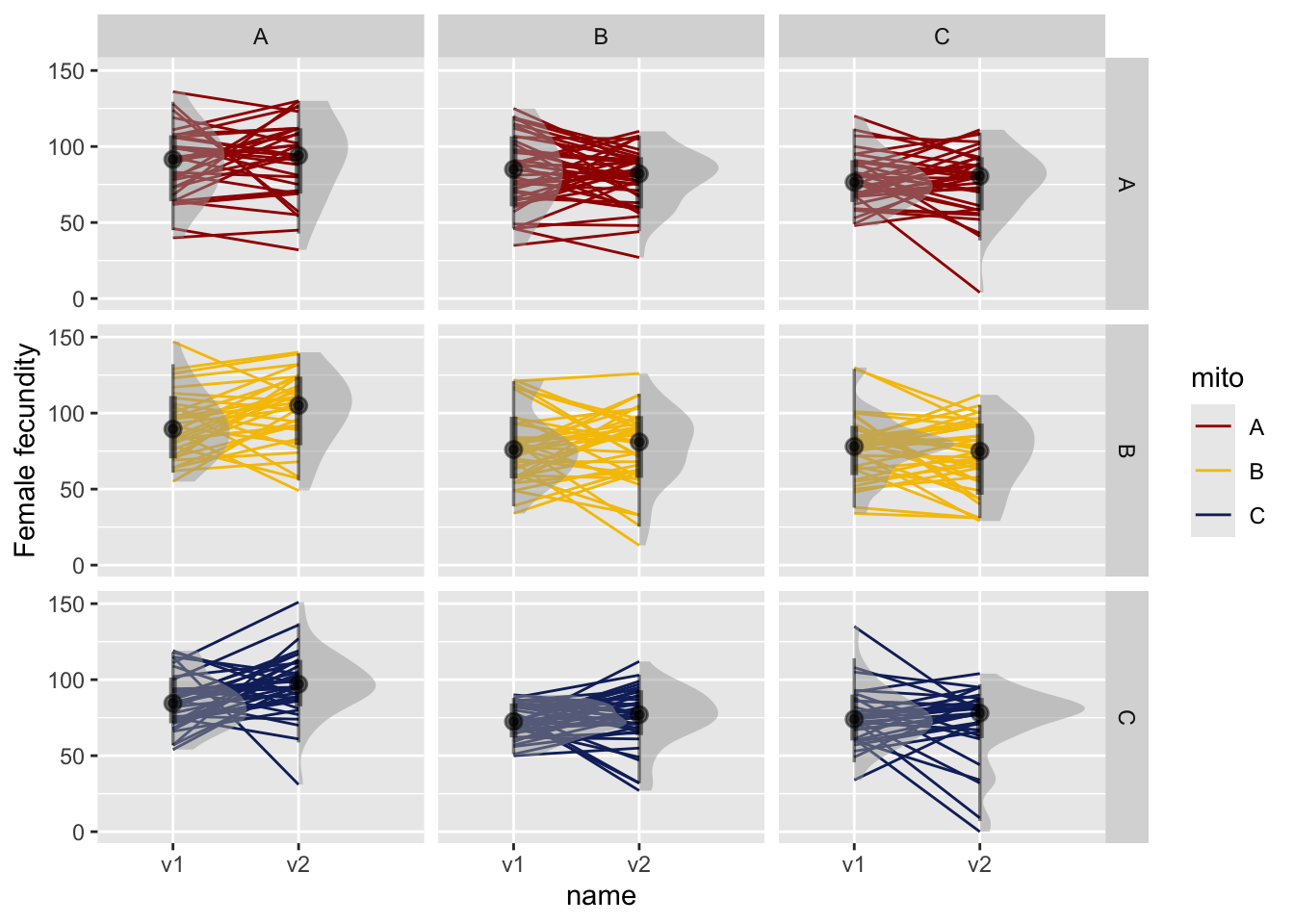

Version	Author	Date
2ee8510	MartinGarlovsky	2024-10-09

Figure 2. Female fecundity in vial 1 and vial 2. Facets are for mito and nuclear genotypes. Lines connect individual females with large points representing the mean and error bars summarise the 66% and 95% quantiles.

# combined vial 1 and vial 2
#hist(daydat$comb_vial)

fecundity_early <- lmerTest::lmer(comb_vial ~ mito * nuclear + (1|LINE), data = daydat, REML = TRUE)

>>> Check diagnostics

performance::check_model(fecundity_early)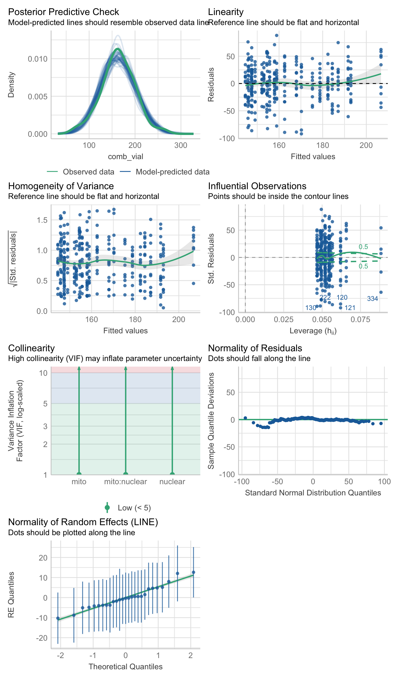

Version	Author	Date
2ee8510	MartinGarlovsky	2024-10-09

anova(fecundity_early, type = "III", ddf = "Kenward-Roger") %>% broom::tidy() %>% 
  as_tibble() %>% 
  kable(digits = 3, 
        caption = 'Type III Analysis of Variance Table with Kenward-Roger`s method') %>% 
  kable_styling(full_width = FALSE)

Type III Analysis of Variance Table with Kenward-Roger`s method
term	sumsq	meansq	NumDF	DenDF	statistic	p.value
mito	1548.543	774.272	2	17.787	0.714	0.503
nuclear	39590.215	19795.107	2	17.765	18.266	0.000
mito:nuclear	3322.807	830.702	4	17.750	0.767	0.561

emmeans(fecundity_early, pairwise ~ nuclear, adjust = "tukey")$contrasts %>% broom::tidy() %>% 
  kable(digits = 3, 
        caption = 'Posthoc Tukey tests for days effect. Results are averaged over the levels of mito') %>% 
  kable_styling(full_width = FALSE)

Posthoc Tukey tests for days effect. Results are averaged over the levels of mito
term	contrast	estimate	std.error	df	statistic	adj.p.value
nuclear	A - B	30.404	6.216	17.556	4.891	0.000
nuclear	A - C	35.172	6.341	18.553	5.547	0.000
nuclear	B - C	4.768	6.222	17.269	0.766	0.728

>>> Matched vs. mismatched

coevo_early <- lmerTest::lmer(comb_vial ~ coevolved + (1|LINE), data = daydat, REML = TRUE)

anova(coevo_early, type = "III", ddf = "Kenward-Roger")

Type III Analysis of Variance Table with Kenward-Roger's method
          Sum Sq Mean Sq NumDF  DenDF F value Pr(>F)
coevolved  509.6   509.6     1 25.442  0.4702 0.4991

>>> Mito-type analysis

fecundity_day1_snp <- lmerTest::lmer(comb_vial ~ mito_snp * nuclear + (1|LINE), data = daydat, REML = TRUE)
anova(fecundity_day1_snp, type = "III", ddf = "Kenward-Roger")

Type III Analysis of Variance Table with Kenward-Roger's method
                  Sum Sq Mean Sq NumDF  DenDF F value  Pr(>F)  
mito_snp          4327.1   540.9     8 8.6615  0.4991 0.82890  
nuclear          15644.0  7822.0     2 9.2612  7.2131 0.01292 *
mito_snp:nuclear 10169.7  1452.8     7 8.9663  1.3398 0.33402  
---
Signif. codes:  0 '***' 0.001 '**' 0.01 '*' 0.05 '.' 0.1 ' ' 1

early_fec_snp <- emmeans(fecundity_day1_snp, ~ mito_snp * nuclear, type = 'response') %>% 
  as_tibble() %>% drop_na() %>% 
  ggplot(aes(x = nuclear, y = emmean, fill = mito_snp)) +
  geom_jitter(data = daydat,
              aes(y = comb_vial, colour = mito_snp),
               position = position_jitterdodge(dodge.width = .5, jitter.width = .1),
              alpha = .25) +
  geom_errorbar(aes(ymin = lower.CL, ymax = upper.CL), 
                width = .25, position = position_dodge(width = .5)) +
  geom_point(size = 3, pch = 21, position = position_dodge(width = .5)) +
  labs(y = 'Early life fecundity (EMM ± 95% CIs)') +
  scale_colour_viridis_d(option = "H") +
  scale_fill_viridis_d(option = "H") +
  theme_bw() + 
  theme() + 
  NULL

early_fec_snp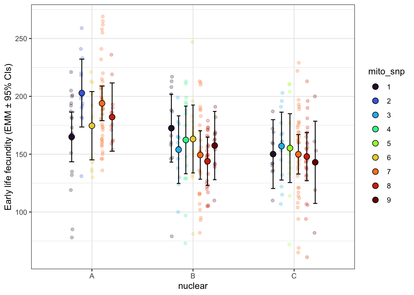

Version	Author	Date
2ee8510	MartinGarlovsky	2024-10-09

> Lifetime fecundity

Here we sum the total number of offspring each female produced across the entire 21 days.

# summarised data 
sum_fecundity <- fert_dat %>% 
  group_by(ID, mito, mito_snp, mtgrp, nuclear, mtn, coevolved, LINE) %>% 
  summarise(total.fec = sum(progeny)) %>% 
  ungroup() %>% 
  mutate(# scale variables 
    scaled_fec = as.numeric(scale(total.fec)),
    # add observation level random effect
    OLRE = 1:nrow(.))

# check mtgrp not crossed within lines
#xtabs(~ LINE + mtgrp, data = sum_fecundity)

hist(sum_fecundity$total.fec, breaks = 50)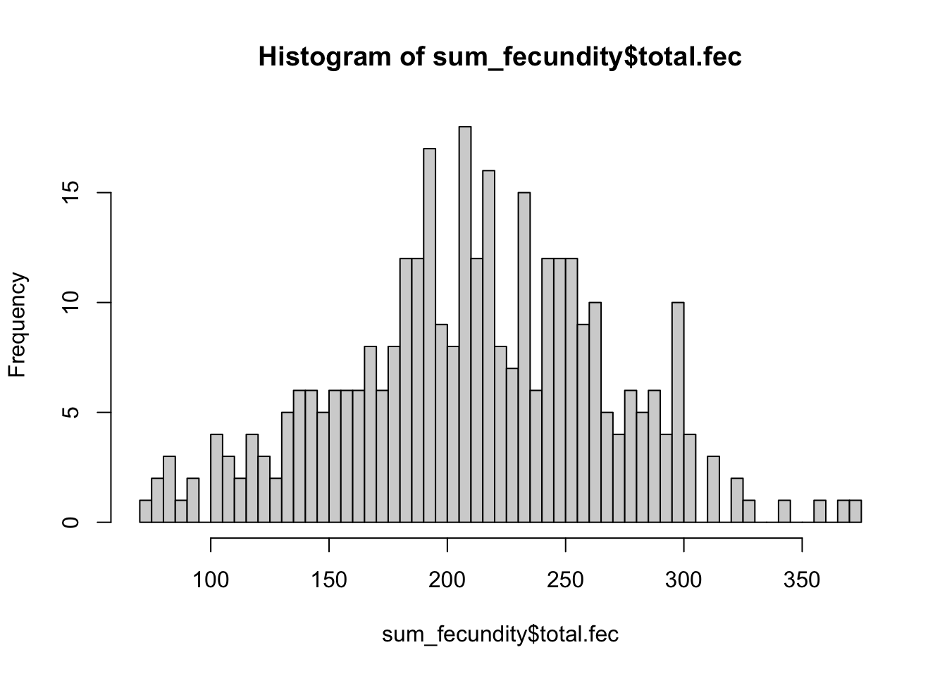

Version	Author	Date
2ee8510	MartinGarlovsky	2024-10-09

# fit linear fit
fecundity_total <- lmerTest::lmer(total.fec ~ mito * nuclear + (1|LINE), data = sum_fecundity, REML = TRUE)

>>> Check diagnostics

performance::check_model(fecundity_total)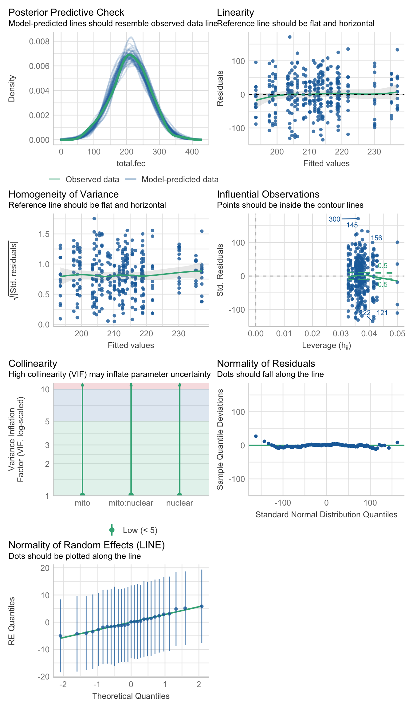

Version	Author	Date
2ee8510	MartinGarlovsky	2024-10-09

anova(fecundity_total, type = "III", ddf = "Kenward-Roger")

Type III Analysis of Variance Table with Kenward-Roger's method
              Sum Sq Mean Sq NumDF  DenDF F value Pr(>F)
mito          2951.2  1475.6     2 17.582  0.4769 0.6285
nuclear       7986.8  3993.4     2 17.533  1.2906 0.3000
mito:nuclear 16005.0  4001.2     4 17.511  1.2931 0.3108

# grand mean
#emmeans::emmeans(fecundity_total, specs = ~1, type = "response")

>>> Matched vs. mismatched

fecundity_coevo <- lmerTest::lmer(total.fec ~ coevolved + (1|LINE), data = sum_fecundity, REML = TRUE)
anova(fecundity_coevo, type = "III", ddf = "Kenward-Roger")

Type III Analysis of Variance Table with Kenward-Roger's method
          Sum Sq Mean Sq NumDF  DenDF F value Pr(>F)
coevolved 2391.7  2391.7     1 25.446  0.7729 0.3875

>>> Mito-type analysis

fecundity_lmer_snp <- lmerTest::lmer(total.fec ~ mito_snp * nuclear + (1|LINE), data = sum_fecundity)
anova(fecundity_lmer_snp, type = "III", ddf = "Kenward-Roger")

Type III Analysis of Variance Table with Kenward-Roger's method
                 Sum Sq Mean Sq NumDF  DenDF F value Pr(>F)
mito_snp          19929  2491.2     8 8.1317  0.8067 0.6154
nuclear              41    20.4     2 9.5863  0.0066 0.9934
mito_snp:nuclear  47266  6752.3     7 8.6974  2.1827 0.1399

lifetime_fec_snp <- emmeans(fecundity_lmer_snp, ~ mito_snp * nuclear) %>% as_tibble() %>% drop_na() %>% 
  ggplot(aes(x = nuclear, y = emmean, fill = mito_snp)) +
  geom_jitter(data = sum_fecundity,
              aes(y = total.fec, colour = mito_snp),
               position = position_jitterdodge(dodge.width = .5, jitter.width = .1),
              alpha = .5) +
  geom_errorbar(aes(ymin = lower.CL, ymax = upper.CL), 
                width = .25, position = position_dodge(width = .5)) +
  geom_point(size = 3, pch = 21, position = position_dodge(width = .5)) +
  labs(y = 'Lifetime fecundity (EMM ± 95% CIs)',
       colour = 'nuclear', fill = 'nuclear') +
  scale_colour_viridis_d(option = "H") +
  scale_fill_viridis_d(option = "H") +
  theme_bw() +
  #theme(legend.position = 'bottom') +
  NULL

lifetime_fec_snp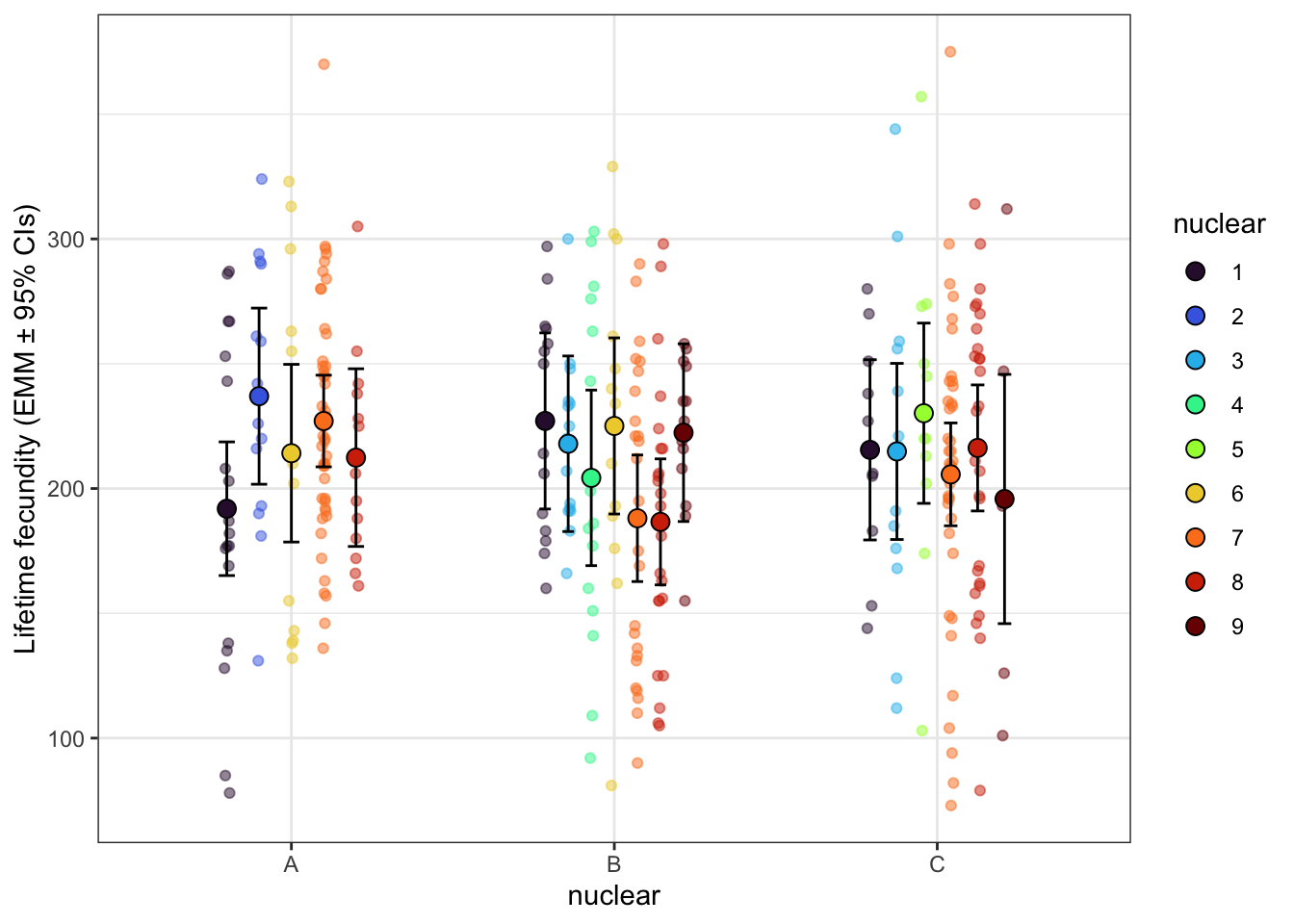

Version	Author	Date
2ee8510	MartinGarlovsky	2024-10-09

> Rate of decline

We modelled the rate of progeny production using a GLMM during the period of decline, namely from vial 2 to 6 (excluding vials 1 and 7). A quick plot of the data suggests a non-linear relationship between progeny production and vial.

fert_filt <- fert_dat %>% filter(vial != '1', vial <= 6)

>> Linear

fert_filt %>% 
  ggplot(aes(x = vial, y = progeny, colour = mito)) +
  geom_point(alpha = .25, position = position_dodge(width = .5)) +
  stat_smooth(method = "lm", formula = y ~ poly(x, 1), colour = "black") +
  facet_wrap(~ nuclear) +
  scale_x_continuous(breaks = c(1:7)) +
  scale_colour_manual(values = met3) +
  scale_fill_manual(values = met3) +
  theme_bw() + 
  theme() + 
  NULL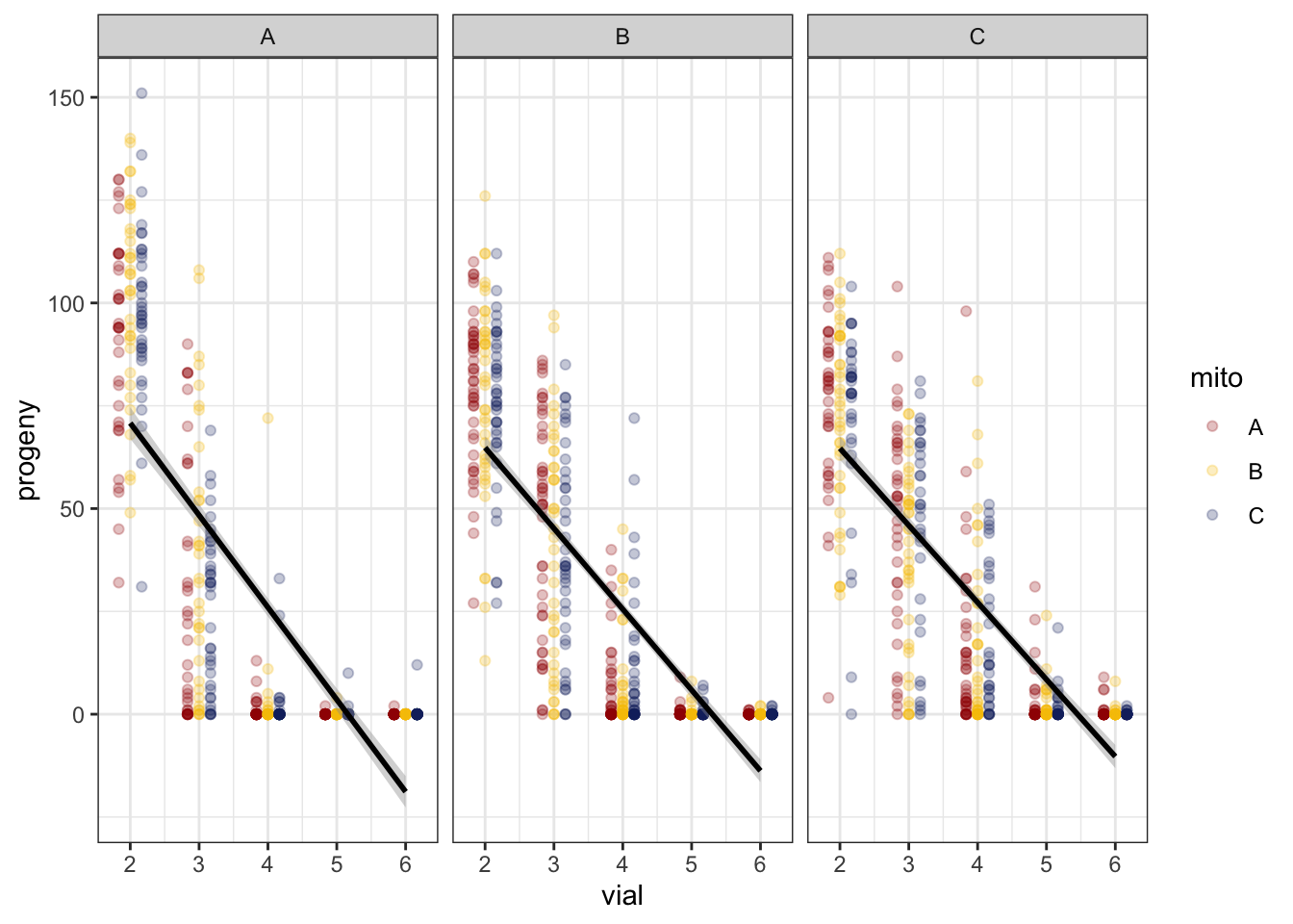

Version	Author	Date
2ee8510	MartinGarlovsky	2024-10-09

>> Polynomial

fert_filt %>% 
  ggplot(aes(x = vial, y = progeny, colour = mito)) +
  geom_point(alpha = .25, position = position_dodge(width = .5)) +
  stat_smooth(method = "lm", formula = y ~ poly(x, 2), colour = "black") +
  facet_wrap(~ nuclear) +
  scale_x_continuous(breaks = c(1:7)) +
  scale_colour_manual(values = met3) +
  scale_fill_manual(values = met3) +
  theme_bw() + 
  theme() + 
  NULL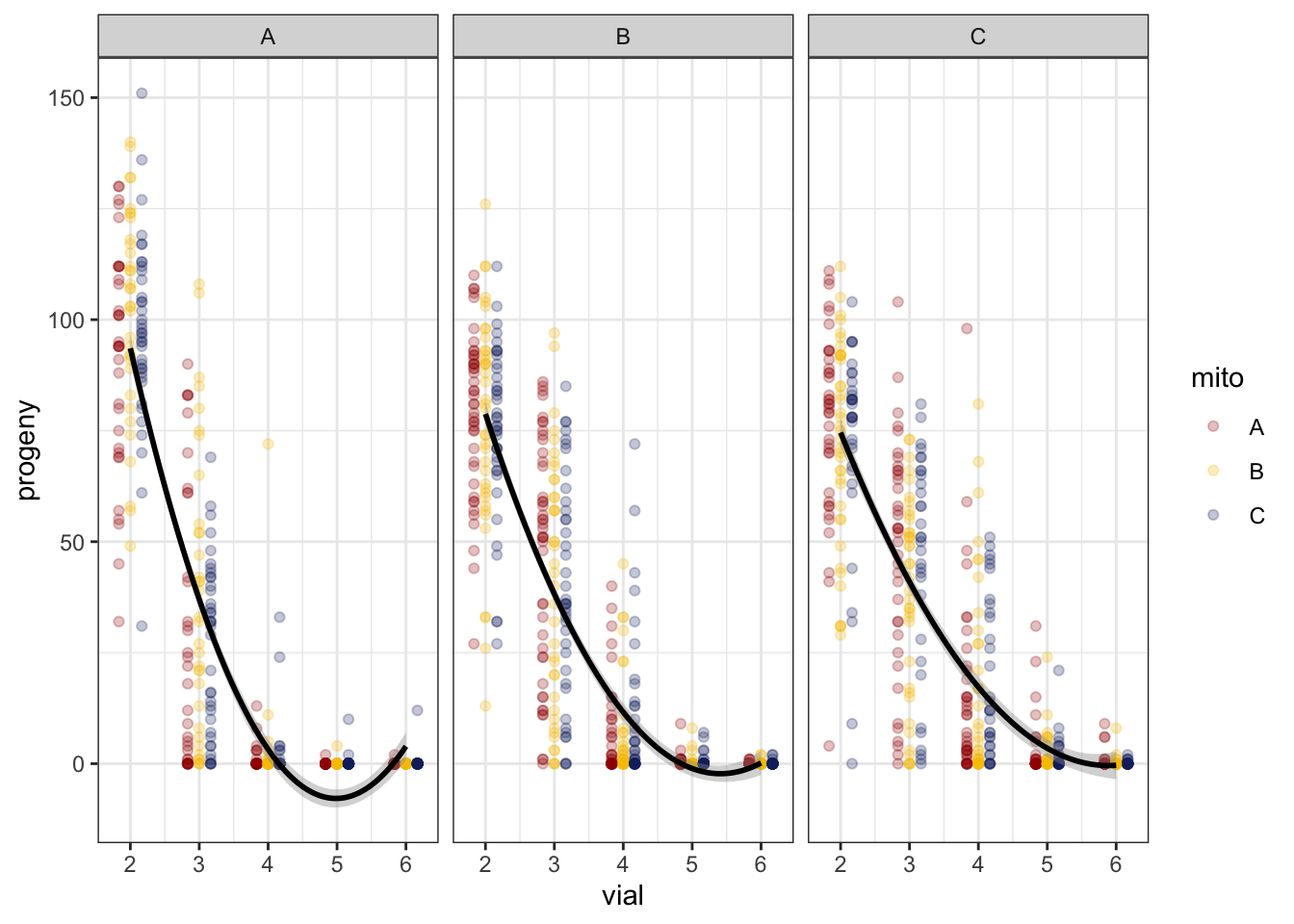

Version	Author	Date
2ee8510	MartinGarlovsky	2024-10-09

>> Fit the model

We compared a linear fit to a polynomial fit. Based on AICc, the second order polynomial fit is preferred.

# fit model
rate_glmm <- glmer(progeny ~ mito * nuclear * vial + (1|LINE:vial) + (1|ID) + (1|OLRE),
                   data = fert_filt, family = 'poisson',
                   control = glmerControl(optimizer = "bobyqa", optCtrl = list(maxfun = 50000)))

# fit model
rate_poly <- glmer(progeny ~ mito * nuclear * vial + I(vial^2) + (1|LINE:vial) + (1|ID) + (1|OLRE),
                   data = fert_filt, family = 'poisson',
                   control = glmerControl(optimizer = "bobyqa", optCtrl = list(maxfun = 50000)))

MuMIn::AICc(rate_glmm, rate_poly)

          df     AICc
rate_glmm 21 9824.599
rate_poly 22 9809.792

>>> Check diagnostics

performance::check_model(rate_poly)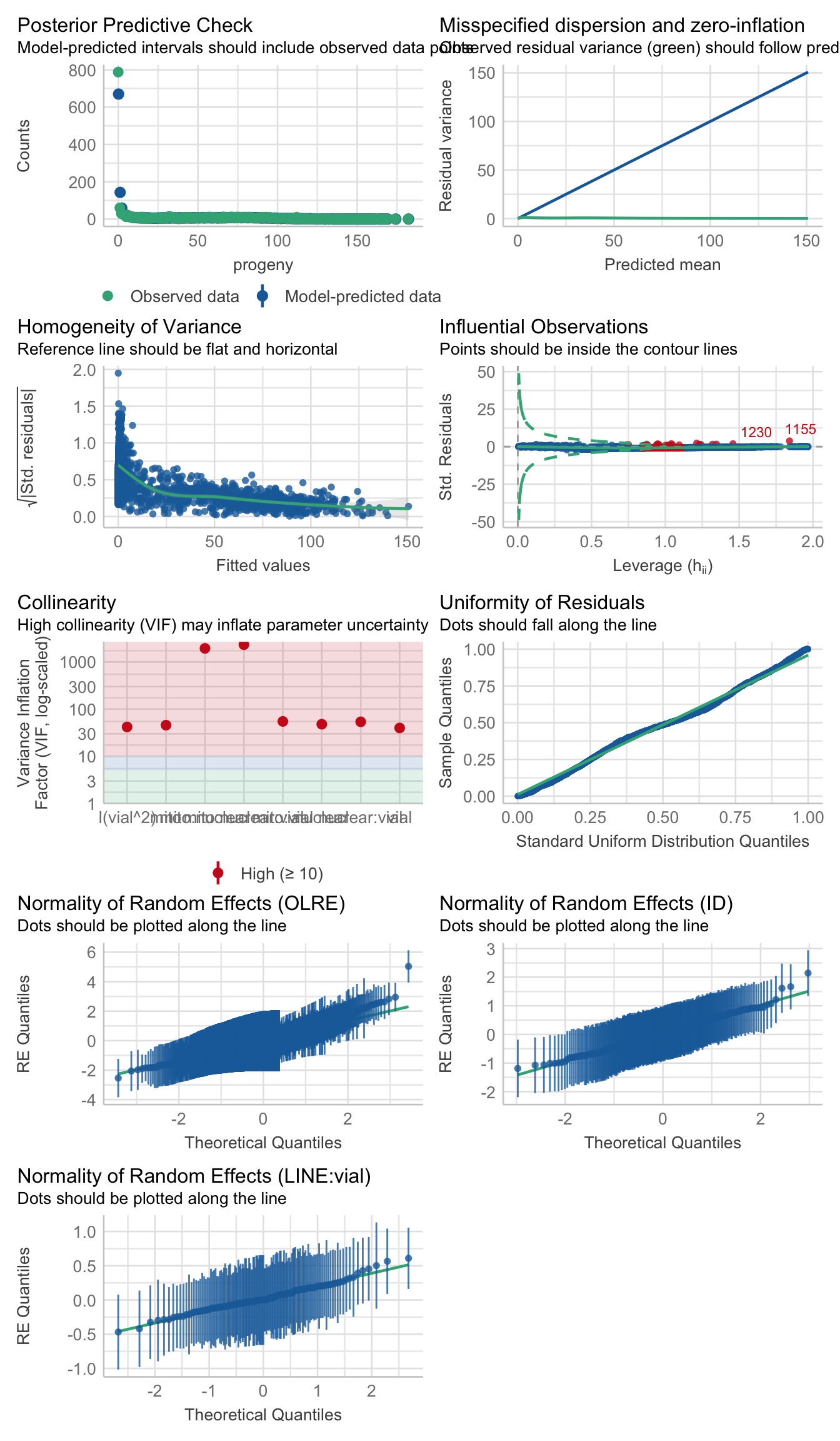

Version	Author	Date
2ee8510	MartinGarlovsky	2024-10-09

performance::check_overdispersion(rate_poly) # not overdispersed

# Overdispersion test

       dispersion ratio =   0.334
  Pearson's Chi-Squared = 557.699
                p-value =       1

performance::check_zeroinflation(rate_poly) # zero inflated

# Check for zero-inflation

   Observed zeros: 788
  Predicted zeros: 669
            Ratio: 0.85

testDispersion(rate_poly)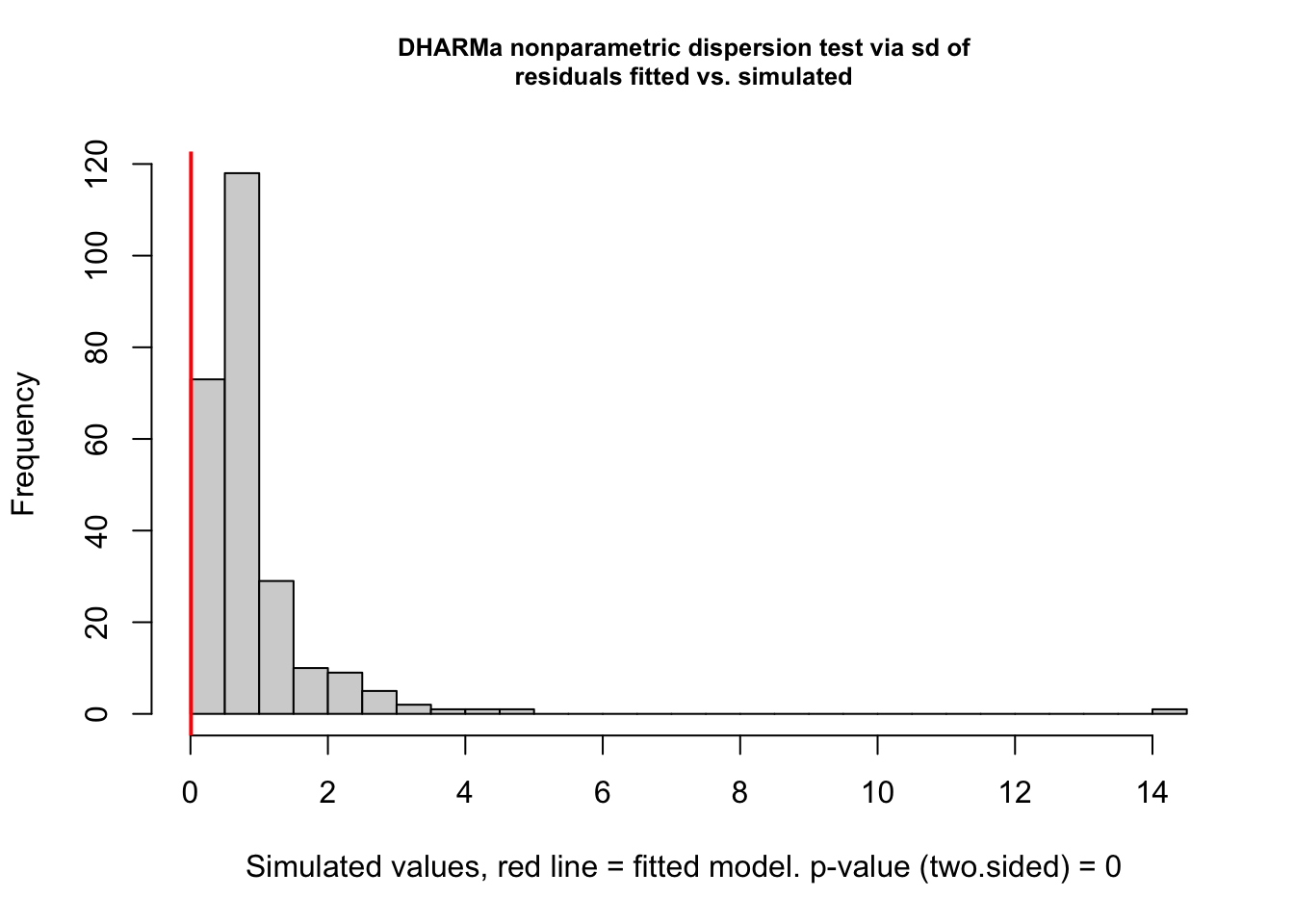

Version	Author	Date
2ee8510	MartinGarlovsky	2024-10-09

    DHARMa nonparametric dispersion test via sd of residuals fitted vs.
    simulated

data:  simulationOutput
dispersion = 0.00862, p-value < 2.2e-16
alternative hypothesis: two.sided

simulationOutput <- simulateResiduals(fittedModel = rate_poly, plot = FALSE)
testZeroInflation(simulationOutput)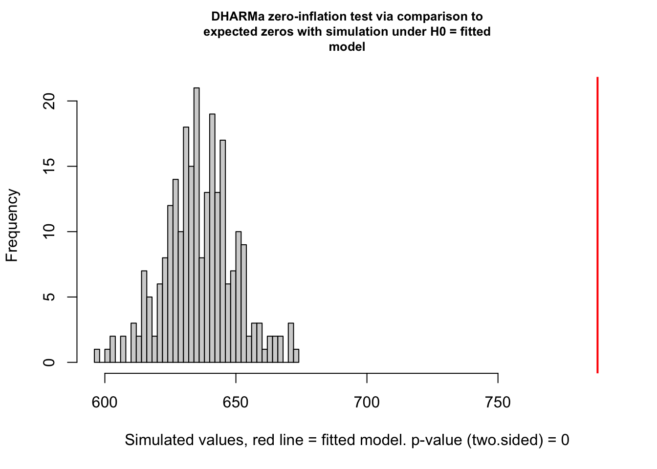

Version	Author	Date
2ee8510	MartinGarlovsky	2024-10-09

    DHARMa zero-inflation test via comparison to expected zeros with
    simulation under H0 = fitted model

data:  simulationOutput
ratioObsSim = 1.2374, p-value < 2.2e-16
alternative hypothesis: two.sided

hist(residuals(simulationOutput))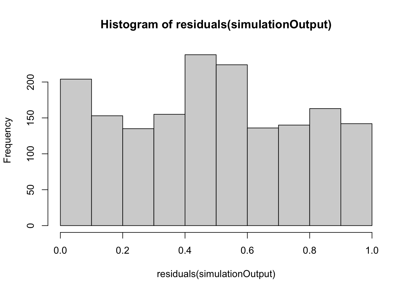

Version	Author	Date
2ee8510	MartinGarlovsky	2024-10-09

hist(residuals(simulationOutput, quantileFunction = qnorm, outlierValues = c(-7,7)))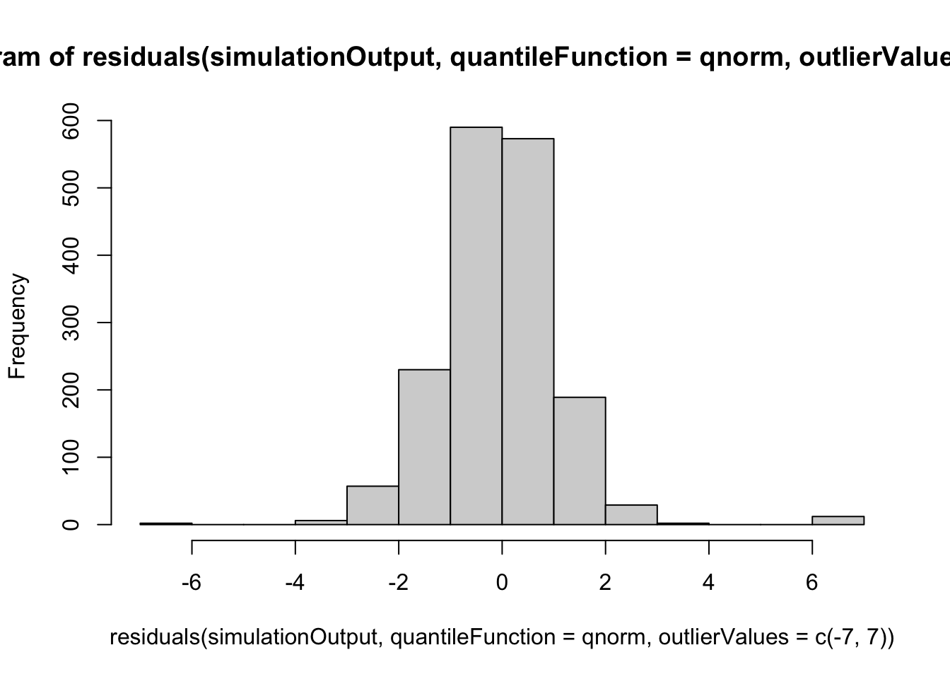

Version	Author	Date
2ee8510	MartinGarlovsky	2024-10-09

plot(simulationOutput)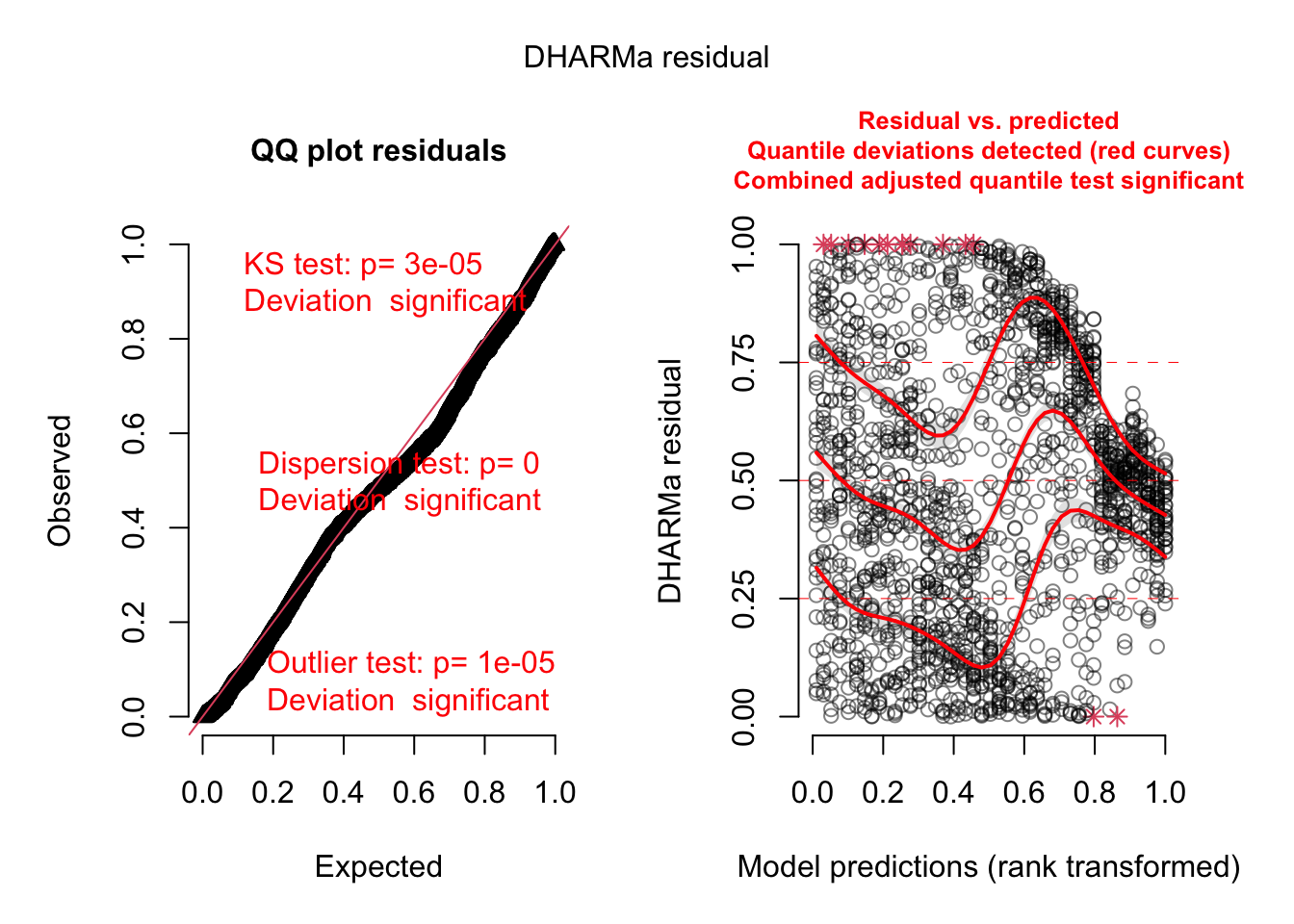

Version	Author	Date
2ee8510	MartinGarlovsky	2024-10-09

>> Results

car::Anova(rate_poly, type = 'III')

Analysis of Deviance Table (Type III Wald chisquare tests)

Response: progeny
                     Chisq Df Pr(>Chisq)    
(Intercept)       221.0932  1  < 2.2e-16 ***
mito                2.1116  2    0.34791    
nuclear            35.7304  2  1.743e-08 ***
vial                9.0479  1    0.00263 ** 
I(vial^2)          19.6275  1  9.411e-06 ***
mito:nuclear        2.6912  4    0.61076    
mito:vial           4.3477  2    0.11374    
nuclear:vial       84.1731  2  < 2.2e-16 ***
mito:nuclear:vial   3.2873  4    0.51095    
---
Signif. codes:  0 '***' 0.001 '**' 0.01 '*' 0.05 '.' 0.1 ' ' 1

#summary(rate_glmm)

emt <- emtrends(rate_poly, "nuclear", var = "vial")
#pairs(emt)

rate_norms <- emtrends(rate_poly, c("mito", "nuclear"), var = "vial") %>% as_tibble() %>% 
  ggplot(aes(x = nuclear, y = vial.trend, fill = mito)) +
  geom_line(aes(group = mito, colour = mito), position = position_dodge(width = .5)) +
  geom_point(size = 3, pch = 21, position = position_dodge(width = .5)) +
  labs(y = 'Fecundity (EMM)') +
  scale_colour_manual(values = met3) +
  scale_fill_manual(values = met3) +
  theme_bw() + 
  theme() + 
  NULL

>>>>> Model predicted values

Here we generate model predicted values for a model with a simplified random effects structure. This is unused in the manuscript at present.

# reduced model for predicted values
# # plot data and model fit
rate_glmm_dummy <- glmer(progeny ~ mito * nuclear * vial + I(vial^2) + (1 + vial|LINE),
                         data = fert_filt, family = 'poisson',
                         control = glmerControl(optimizer = "bobyqa", optCtrl = list(maxfun = 50000)))

#car::Anova(rate_glmm_dummy, type = 'III')

prediction_data <- expand.grid(vial = seq(from = 2, to = 6, length = 100), 
                               #ID = unique(fert_filt$ID),
                               #OLRE = unique(fert_filt$OLRE),
                               LINE = levels(as.factor(fert_filt$LINE))) %>%
  mutate(mito = str_sub(LINE, 1, 1),
         nuclear = str_sub(LINE, 2, 2))

mySumm <- function(.) {
  predict(., newdata=prediction_data, re.form=NULL)
}
####Collapse bootstrap into median, 95% PI
sumBoot <- function(merBoot) {
  return(
    data.frame(fit = apply(merBoot$t, 2, function(x) as.numeric(quantile(x, probs=.5, na.rm=TRUE))),
               lwr = apply(merBoot$t, 2, function(x) as.numeric(quantile(x, probs=.025, na.rm=TRUE))),
               upr = apply(merBoot$t, 2, function(x) as.numeric(quantile(x, probs=.975, na.rm=TRUE)))
    )
  )
}

### Reader beware - this takes a long time to run!!!
##lme4::bootMer() method 2
# PI.boot2.time <- system.time(
#   boot2 <- lme4::bootMer(rate_glmm_dummy, mySumm, nsim=1000, use.u=TRUE, type="parametric", .progress = "txt")
# )
##saveRDS(boot2, file = "output/female_rates_poly.Rdata")

boot2 <- read_rds("output/female_rates_poly.Rdata")
PI.boot2 <- sumBoot(boot2)

plot_data <- data.frame(prediction_data, PI.boot2)
#head(plot_data)
colnames(plot_data)[5] <- "progeny"

plot_data_summary <- plot_data %>% 
  group_by(mito, nuclear, vial) %>% 
  summarise(mn_fit = mean(progeny),
            #mn_sef = mean(se.fit),
            mn_lwr = mean(lwr),
            mn_upr = mean(upr)
            ) %>% 
  ungroup() %>% mutate(across(4:6, ~exp(.x)))

# plot
fert_mns <- fert_filt %>% 
  group_by(mito, nuclear, vial) %>% 
  summarise(mn = mean(progeny),
            se = sd(progeny)/sqrt(n()),
            s95 = se * 1.96)

rateP <- fert_filt %>% 
  ggplot(aes(x = vial, y = progeny, colour = mito)) +
  geom_point(aes(y = progeny, colour = mito, shape = mito), alpha = .15,
             position = position_jitterdodge(dodge.width = .5, jitter.width = .1)) +
  geom_ribbon(data = plot_data_summary,
              aes(y = mn_fit, ymin = mn_lwr, ymax = mn_upr, fill = mito, group = mito),
              alpha = .5, colour = NA) +
  geom_line(data = plot_data_summary,
            aes(y = mn_fit, colour = mito, group = mito)) +
  geom_errorbar(data = fert_mns,
                aes(y = mn, ymin = mn - s95, ymax = mn + s95),
                width = .25, position = position_dodge(width = .5)) +
  geom_point(data = fert_mns, aes(y = mn), position = position_dodge(width = .5)) +
  scale_x_continuous(breaks = c(1:7)) +
  scale_colour_manual(values = met3) +
  scale_fill_manual(values = met3) +
  labs(y = 'Fecundity per vial (mean ± SE)') +
  facet_wrap(~ nuclear) + 
  theme_bw() + 
  theme() + 
  #ggsave('figures/vial_means.pdf', height = 3, width = 9, dpi = 600, useDingbats = FALSE) +
  NULL

rateP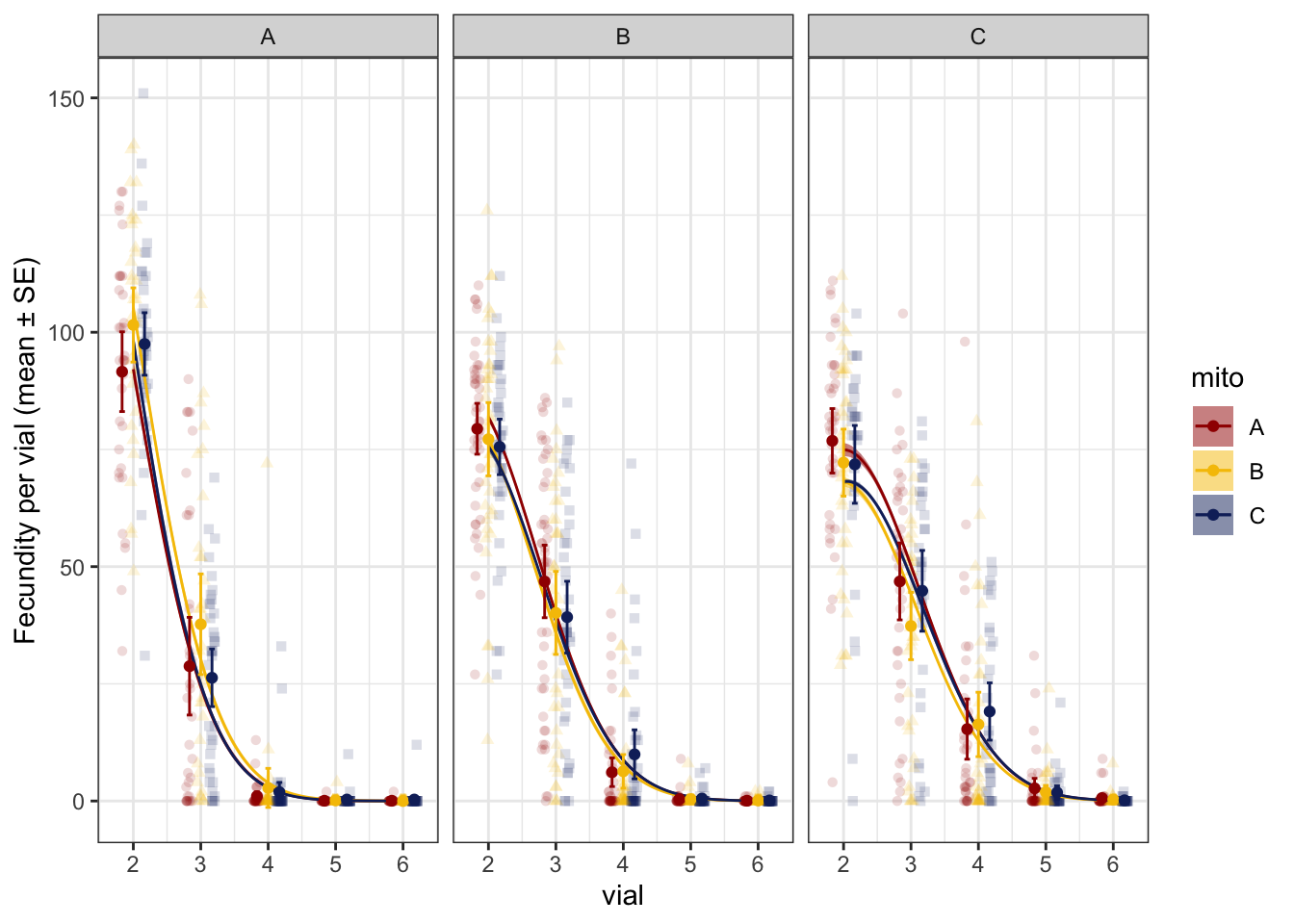

Version	Author	Date
2ee8510	MartinGarlovsky	2024-10-09

# raw data
fem_fert_rawplot <- fert_dat %>% 
  group_by(mito, nuclear, vial) %>% 
  summarise(mn = mean(progeny),
            se = sd(progeny)/sqrt(n()),
            s95 = se * 1.96) %>% 
  ggplot(aes(x = vial, y = mn, colour = mito)) +
  geom_point(data = fert_dat,
             aes(y = progeny, colour = mito), alpha = .15,
             position = position_jitterdodge(dodge.width = .5, jitter.width = .1)) +
  geom_errorbar(aes(ymin = mn - s95, ymax = mn + s95), 
                width = .25, position = position_dodge(width = .5)) +
  geom_point(position = position_dodge(width = .5)) +
  scale_x_continuous(breaks = c(1:7)) +
  scale_colour_manual(values = met3) +
  scale_fill_manual(values = met3) +
  labs(y = 'Fecundity per vial (mean ± SE)') +
  facet_wrap(~ nuclear) +
  theme_bw() + 
  theme() + 
  NULL
#ggsave(filename = 'figures/fem_fert_rawplot.pdf', height = 4, width = 9, dpi = 600, useDingbats = FALSE)

>>> Matched vs. mismatched

rate_coevo <- glmer(progeny ~ coevolved * vial + (1|LINE:vial) + (1|ID) + (1|OLRE),
                         data = fert_filt, family = 'poisson',
                         control = glmerControl(optimizer = "bobyqa", optCtrl = list(maxfun = 50000)))

car::Anova(rate_coevo, type = 'III')

Analysis of Deviance Table (Type III Wald chisquare tests)

Response: progeny
                   Chisq Df Pr(>Chisq)    
(Intercept)    1135.0369  1     <2e-16 ***
coevolved         0.0319  1     0.8581    
vial            885.9213  1     <2e-16 ***
coevolved:vial    0.0069  1     0.9338    
---
Signif. codes:  0 '***' 0.001 '**' 0.01 '*' 0.05 '.' 0.1 ' ' 1

>>> Mito-type analysis

# fit model
rate_glmm_snp <- glmer(progeny ~ mito_snp * nuclear * vial + (1|LINE:vial) + (1|ID) + (1|OLRE),
                       data = fert_filt, family = 'poisson', 
                       control= glmerControl(optimizer="bobyqa", optCtrl=list(maxfun=50000)))

car::Anova(rate_glmm_snp, type = 'III')

Analysis of Deviance Table (Type III Wald chisquare tests)

Response: progeny
                         Chisq Df Pr(>Chisq)    
(Intercept)           157.6550  1    < 2e-16 ***
mito_snp                6.5879  8    0.58168    
nuclear                 0.2651  2    0.87588    
vial                  117.0384  1    < 2e-16 ***
mito_snp:nuclear        5.1144  7    0.64600    
mito_snp:vial          13.9589  8    0.08284 .  
nuclear:vial            2.6662  2    0.26366    
mito_snp:nuclear:vial   9.3443  7    0.22887    
---
Signif. codes:  0 '***' 0.001 '**' 0.01 '*' 0.05 '.' 0.1 ' ' 1

#summary(rate_glmm_snp)

> Combined plot for all stages

comb_all_female <- bind_rows(
  emmeans(fecundity_early, ~ mito * nuclear) %>% as_tibble() %>% mutate(stage = "a) Early life"),
  emmeans(fecundity_total, ~ mito * nuclear) %>% as_tibble() %>% mutate(stage = "b) Lifetime"),
  emtrends(rate_glmm, c("mito", "nuclear"), var = "vial") %>% as_tibble() %>% 
    mutate(stage = "c) Rate of decline",
           emmean = vial.trend)) %>% 
  ggplot(aes(x = nuclear, y = emmean, fill = mito)) +
  geom_line(aes(group = mito, colour = mito), position = position_dodge(width = .5)) +
  geom_point(size = 3, pch = 21, position = position_dodge(width = .5)) +
  labs(y = 'Fecundity (EMM)') +
  scale_colour_manual(values = met3) +
  scale_fill_manual(values = met3) +
  facet_wrap(~stage, scales = "free_y") +
  theme_bw() + 
  theme() + 
  NULL

comb_all_female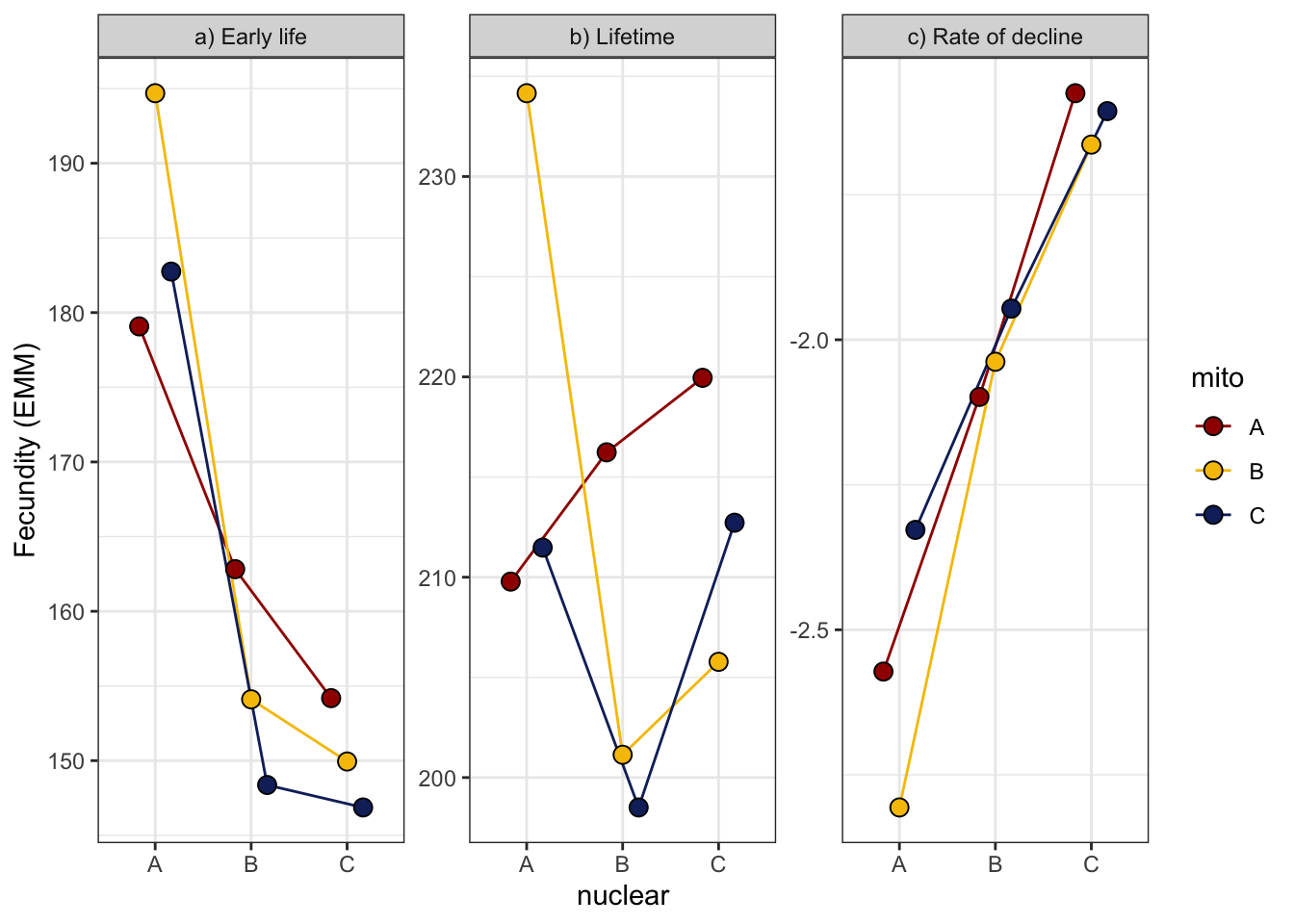

Version	Author	Date
2ee8510	MartinGarlovsky	2024-10-09

#ggsave(filename = 'figures/femaleplot_norms3.pdf', height = 4, width = 12, dpi = 600, useDingbats = FALSE)

> Survival analysis

Finally, we modelled reproductive senescence using survival analysis based on the onset of infertility, i.e., the time (in vials) to event (final vial producing progeny for each female) as the response.

library(coxme)
library(survminer)

fsurv <- fert_dat %>% 
  mutate(bin_prog = if_else(progeny == 0, 0, 1),
         mito_snp = as.factor(mito_snp))

fsurv$cum_pr <- ave(fsurv$progeny, fsurv$ID, FUN = cumsum)
fsurv <- fsurv %>% group_by(ID) %>% slice(which.min(progeny)) %>% mutate(EVENT = 1)

fit1 <- survfit(Surv(vial, EVENT) ~ mito + nuclear, data = fsurv)
#summary(fit1)
#anova(fit1)

survplot <- ggsurvplot(fit1, colour = "mito",
                       palette = rep(rev(met3), 3))

survplot$plot + 
  facet_wrap(~nuclear) + 
  theme_bw() + 
  theme(legend.position = "") +
  NULL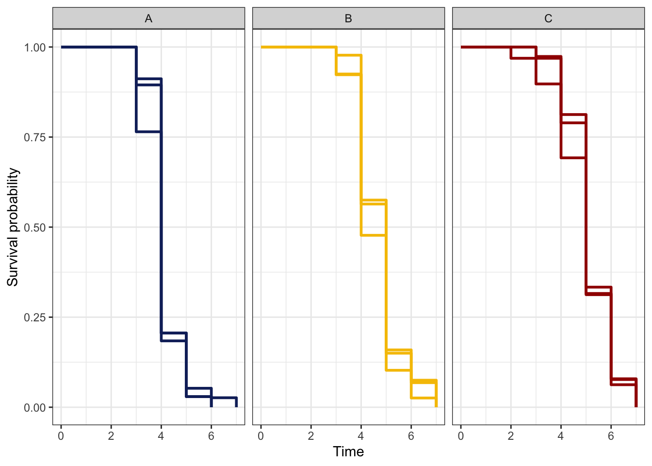

Version	Author	Date
2ee8510	MartinGarlovsky	2024-10-09

>>> Check diagnostics

Using a simplified model without the random effects we can check the proportional hazards assumption.

plot(survfit(Surv(vial, EVENT) ~ mito + nuclear, data = fsurv), 
     lty = 1:4, 
     fun="cloglog", main = "cloglog")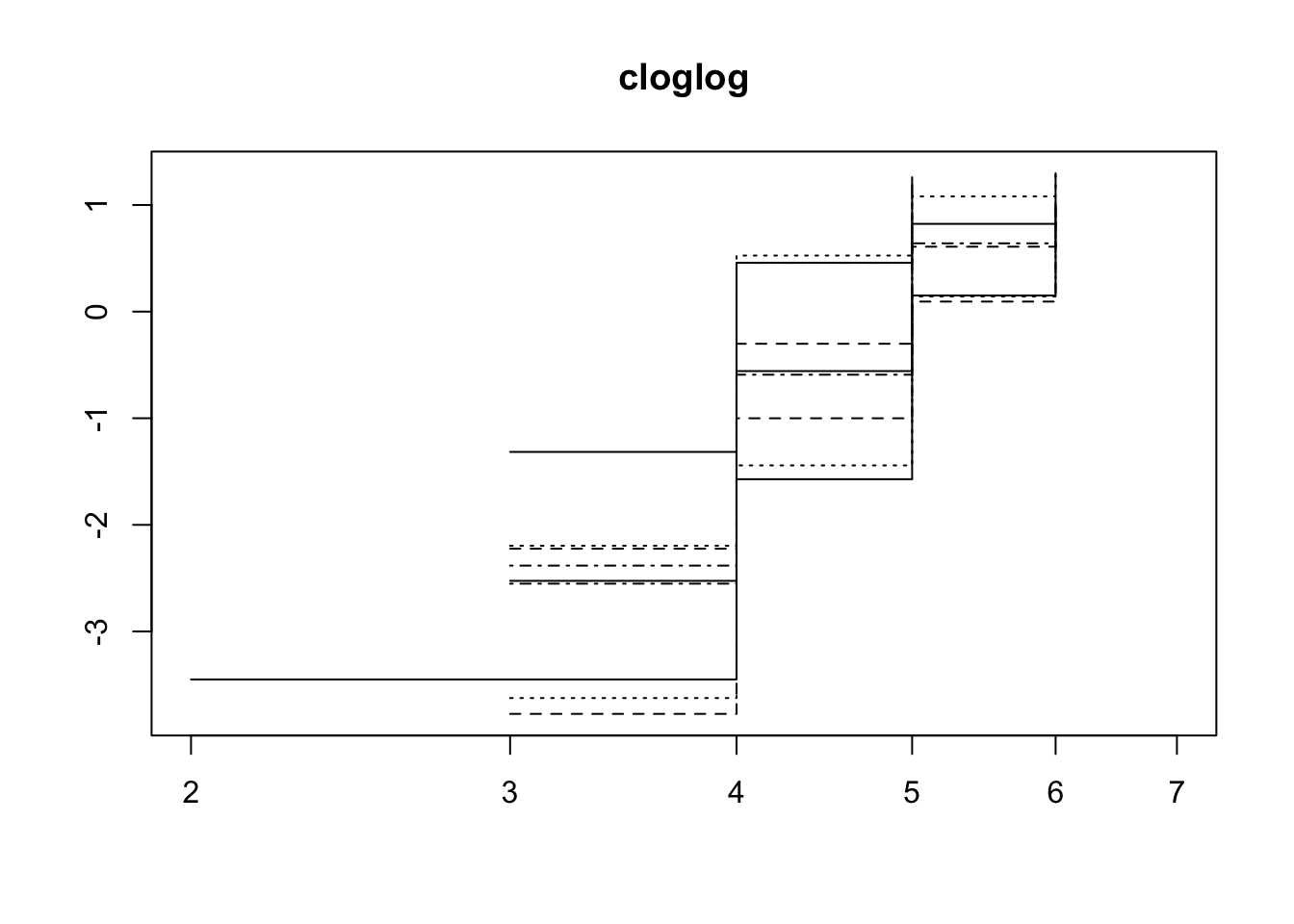

Version	Author	Date
2ee8510	MartinGarlovsky	2024-10-09

test.ph <- cox.zph(coxph(Surv(vial, EVENT) ~ mito * nuclear, data = fsurv))

ggcoxzph(test.ph)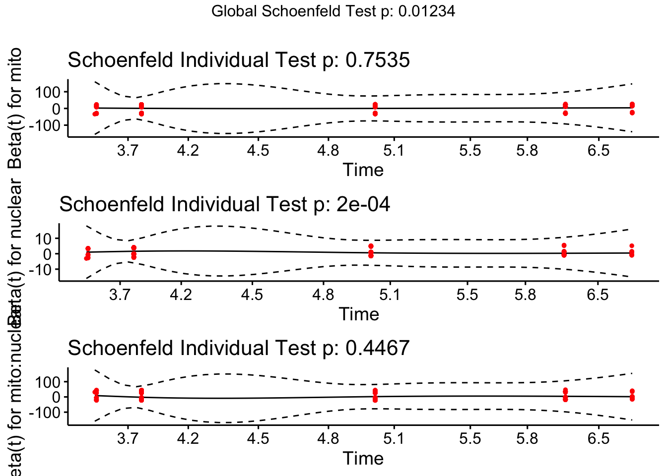

Version	Author	Date
2ee8510	MartinGarlovsky	2024-10-09

We then use likelihood ratio tests comparing the full model to submodels excluding the effect of interest.

cox.des <- coxme(Surv(vial, EVENT) ~ mito * nuclear + (1|LINE), data = fsurv)

cox.des.n1 <- coxme(Surv(vial, EVENT) ~ 1 + nuclear + (1|LINE), data = fsurv)
cox.des.n2 <- coxme(Surv(vial, EVENT) ~ mito + 1 + (1|LINE), data = fsurv)
cox.des.n3 <- coxme(Surv(vial, EVENT) ~ mito + nuclear + (1|LINE), data = fsurv)

# posthoc tests
bind_rows(anova(cox.des, cox.des.n1) %>% broom::tidy(),
          anova(cox.des, cox.des.n2) %>% broom::tidy(),
          anova(cox.des, cox.des.n3) %>% broom::tidy()) %>% #drop_na() %>% 
  kable(digits = 3, 
        caption = 'Likelihood ratio tests comparing the full model to submodels excluding the main effect of interest') %>% 
  kable_styling(full_width = FALSE) %>%
  kableExtra::group_rows("Mitochondria", 1, 2) %>%
  kableExtra::group_rows("Nuclear", 3, 4) %>%
  kableExtra::group_rows("Mitonuclear interaction", 5, 6)

Likelihood ratio tests comparing the full model to submodels excluding the main effect of interest
term	logLik	statistic	df	p.value
Mitochondria
~mito * nuclear + (1 \| LINE)	-1605.899	NA	NA	NA
~1 + nuclear + (1 \| LINE)	-1606.570	1.341	6	0.969
Nuclear
~mito * nuclear + (1 \| LINE)	-1605.899	NA	NA	NA
~mito + 1 + (1 \| LINE)	-1627.989	44.180	6	0.000
Mitonuclear interaction
~mito * nuclear + (1 \| LINE)	-1605.899	NA	NA	NA
~mito + nuclear + (1 \| LINE)	-1606.201	0.603	4	0.963

cox_emm <- emmeans(cox.des, ~ mito * nuclear)

# posthoc tests
emmeans(cox_emm, pairwise ~ nuclear, adjust = "tukey")

$emmeans
 nuclear emmean     SE  df asymp.LCL asymp.UCL
 A        0.610 0.0840 Inf     0.446    0.7749
 B       -0.103 0.0723 Inf    -0.245    0.0387
 C       -0.473 0.0811 Inf    -0.632   -0.3138

Results are averaged over the levels of: mito 
Results are given on the log (not the response) scale. 
Confidence level used: 0.95 

$contrasts
 contrast estimate    SE  df z.ratio p.value
 A - B       0.713 0.136 Inf   5.254  <.0001
 A - C       1.083 0.142 Inf   7.601  <.0001
 B - C       0.370 0.133 Inf   2.786  0.0147

Results are averaged over the levels of: mito 
Results are given on the log (not the response) scale. 
P value adjustment: tukey method for comparing a family of 3 estimates

#emmeans(cox_emm, pairwise ~ nuclear, adjust = "tukey", type = "response")

# posthoc tests
bind_rows(emmeans(cox_emm, pairwise ~ nuclear, adjust = "tukey")$contrasts %>% broom::tidy(),
          emmeans(cox_emm, pairwise ~ nuclear, adjust = "tukey", type = "response")$contrasts %>% broom::tidy()) %>% 
  kable(digits = 3, 
        caption = 'Posthoc Tukey tests to compare which groups differ. Results are averaged over the levels of mito') %>% 
  kable_styling(full_width = FALSE) %>%
  kableExtra::group_rows("log scale", 1, 3) %>%
  kableExtra::group_rows("Hazard ratios", 4, 6)

Posthoc Tukey tests to compare which groups differ. Results are averaged over the levels of mito
term	contrast	null.value	estimate	std.error	df	statistic	adj.p.value	ratio	null
log scale
nuclear	A - B	0	0.713	0.136	Inf	5.254	0.000	NA	NA
nuclear	A - C	0	1.083	0.142	Inf	7.601	0.000	NA	NA
nuclear	B - C	0	0.370	0.133	Inf	2.786	0.015	NA	NA
Hazard ratios
nuclear	A / B	0	NA	0.277	Inf	5.254	0.000	2.041	1
nuclear	A / C	0	NA	0.421	Inf	7.601	0.000	2.954	1
nuclear	B / C	0	NA	0.192	Inf	2.786	0.015	1.447	1

>>> Matched vs. mismatched

cox.coevo <- coxme(Surv(vial, EVENT) ~ coevolved + (1|LINE), data = fsurv)

#anova(cox.coevo)
summary(cox.coevo)

Mixed effects coxme model
 Formula: Surv(vial, EVENT) ~ coevolved + (1 | LINE) 
    Data: fsurv 

  events, n = 338, 338

Random effects:
  group  variable        sd  variance
1  LINE Intercept 0.3747831 0.1404624
                  Chisq    df         p   AIC    BIC
Integrated loglik 12.13  2.00 2.320e-03  8.13   0.49
 Penalized loglik 54.41 16.58 6.524e-06 21.24 -42.15

Fixed effects:
              coef exp(coef) se(coef)   z     p
coevolved1 0.04908   1.05030  0.09776 0.5 0.616

cox.coevo.n1 <- coxme(Surv(vial, EVENT) ~ 1 + (1|LINE), data = fsurv)

anova(cox.coevo, cox.coevo.n1) # mito NS

Analysis of Deviance Table
 Cox model: response is  Surv(vial, EVENT)
 Model 1: ~coevolved + (1 | LINE)
 Model 2: ~1 + (1 | LINE)
   loglik  Chisq Df P(>|Chi|)
1 -1628.0                    
2 -1628.1 0.2392  1    0.6248

>>> Mito-type analysis

The mito-type analysis throws an error due to the rank deficiency of the design.

# cox.snp <- coxme(Surv(vial, EVENT) ~ mito_snp * nuclear + (1|LINE), data = fsurv)
# 
# summary(cox.snp)
# 
# cox.snp.n1 <- coxme(Surv(vial, EVENT) ~ 1 + nuclear + (1|LINE), data = fsurv)
# cox.snp.n2 <- coxme(Surv(vial, EVENT) ~ mito_snp + 1 + (1|LINE), data = fsurv)
# cox.snp.n3 <- coxme(Surv(vial, EVENT) ~ mito_snp + nuclear + (1|LINE), data = fsurv)
# 
# anova(cox.snp, cox.snp.n1) # mito NS
# anova(cox.snp, cox.snp.n2) # nuclear sig
# anova(cox.snp, cox.snp.n3) # interaction NS

sessionInfo()

R version 4.4.0 (2024-04-24)
Platform: aarch64-apple-darwin20
Running under: macOS Sonoma 14.6.1

Matrix products: default
BLAS:   /Library/Frameworks/R.framework/Versions/4.4-arm64/Resources/lib/libRblas.0.dylib 
LAPACK: /Library/Frameworks/R.framework/Versions/4.4-arm64/Resources/lib/libRlapack.dylib;  LAPACK version 3.12.0

locale:
[1] en_US.UTF-8/en_US.UTF-8/en_US.UTF-8/C/en_US.UTF-8/en_US.UTF-8

time zone: Europe/London
tzcode source: internal

attached base packages:
[1] stats     graphics  grDevices utils     datasets  methods   base     

other attached packages:
 [1] survminer_0.4.9  ggpubr_0.6.0     coxme_2.2-22     bdsmatrix_1.3-7 
 [5] survival_3.7-0   conflicted_1.2.0 showtext_0.9-7   showtextdb_3.0  
 [9] sysfonts_0.8.9   knitrhooks_0.0.4 knitr_1.48       kableExtra_1.4.0
[13] emmeans_1.10.4   DHARMa_0.4.6     lme4_1.1-35.5    Matrix_1.7-0    
[17] lubridate_1.9.3  forcats_1.0.0    stringr_1.5.1    dplyr_1.1.4     
[21] purrr_1.0.2      readr_2.1.5      tidyr_1.3.1      tibble_3.2.1    
[25] ggplot2_3.5.1    tidyverse_2.0.0  workflowr_1.7.1 

loaded via a namespace (and not attached):
  [1] tensorA_0.36.2.1     rstudioapi_0.16.0    jsonlite_1.8.9      
  [4] datawizard_0.13.0    magrittr_2.0.3       estimability_1.5.1  
  [7] farver_2.1.2         nloptr_2.1.1         rmarkdown_2.28      
 [10] fs_1.6.4             vctrs_0.6.5          MetBrewer_0.2.0     
 [13] memoise_2.0.1        minqa_1.2.8          rstatix_0.7.2       
 [16] htmltools_0.5.8.1    distributional_0.5.0 broom_1.0.7         
 [19] tidybayes_3.0.7      Formula_1.2-5        sass_0.4.9          
 [22] bslib_0.8.0          pbkrtest_0.5.3       plyr_1.8.9          
 [25] zoo_1.8-12           cachem_1.1.0         whisker_0.4.1       
 [28] mime_0.12            lifecycle_1.0.4      iterators_1.0.14    
 [31] pkgconfig_2.0.3      gap_1.6              R6_2.5.1            
 [34] fastmap_1.2.0        shiny_1.9.1          rbibutils_2.3       
 [37] digest_0.6.37        numDeriv_2016.8-1.1  colorspace_2.1-1    
 [40] patchwork_1.3.0      ps_1.8.0             rprojroot_2.0.4     
 [43] qgam_1.3.4           labeling_0.4.3       km.ci_0.5-6         
 [46] fansi_1.0.6          timechange_0.3.0     httr_1.4.7          
 [49] abind_1.4-8          mgcv_1.9-1           compiler_4.4.0      
 [52] bit64_4.5.2          withr_3.0.1          doParallel_1.0.17   
 [55] backports_1.5.0      carData_3.0-5        performance_0.12.3  
 [58] highr_0.11           ggsignif_0.6.4       MASS_7.3-61         
 [61] tools_4.4.0          httpuv_1.6.15        glue_1.8.0          
 [64] callr_3.7.6          nlme_3.1-166         promises_1.3.0      
 [67] grid_4.4.0           checkmate_2.3.2      getPass_0.2-4       
 [70] see_0.9.0            generics_0.1.3       gtable_0.3.5        
 [73] KMsurv_0.1-5         tzdb_0.4.0           data.table_1.16.0   
 [76] hms_1.1.3            car_3.1-3            xml2_1.3.6          
 [79] utf8_1.2.4           ggrepel_0.9.6        foreach_1.5.2       
 [82] pillar_1.9.0         ggdist_3.3.2         vroom_1.6.5         
 [85] posterior_1.6.0      later_1.3.2          splines_4.4.0       
 [88] lattice_0.22-6       bit_4.5.0            tidyselect_1.2.1    
 [91] git2r_0.33.0         gridExtra_2.3        arrayhelpers_1.1-0  
 [94] svglite_2.1.3        stats4_4.4.0         xfun_0.48           
 [97] MuMIn_1.48.4         stringi_1.8.4        yaml_2.3.10         
[100] boot_1.3-31          codetools_0.2-20     evaluate_1.0.0      
[103] cli_3.6.3            xtable_1.8-4         systemfonts_1.1.0   
[106] Rdpack_2.6.1         munsell_0.5.1        processx_3.8.4      
[109] jquerylib_0.1.4      survMisc_0.5.6       Rcpp_1.0.13         
[112] coda_0.19-4.1        svUnit_1.0.6         parallel_4.4.0      
[115] bayestestR_0.14.0    gap.datasets_0.0.6   viridisLite_0.4.2   
[118] mvtnorm_1.3-1        lmerTest_3.1-3       scales_1.3.0        
[121] insight_0.20.5       crayon_1.5.3         rlang_1.1.4

Female fertility

Martin Garlovsky

2022-08-03

Load packages

Load data

Introduction

> Early life fecundity

>>> Check diagnostics

>>> Matched vs. mismatched

>>> Mito-type analysis

> Lifetime fecundity

>>> Check diagnostics

>>> Matched vs. mismatched

>>> Mito-type analysis

> Rate of decline

>> Linear

>> Polynomial

>> Fit the model

>>> Check diagnostics

>> Results

>>>>> Model predicted values

>>> Matched vs. mismatched

>>> Mito-type analysis

> Combined plot for all stages

> Survival analysis

>>> Check diagnostics

>>> Matched vs. mismatched

>>> Mito-type analysis