Basic Operations with Raster Data
Last updated: 2024-12-28
Checks: 7 0
Knit directory: R_tutorial/
This reproducible R Markdown analysis was created with workflowr (version 1.7.1). The Checks tab describes the reproducibility checks that were applied when the results were created. The Past versions tab lists the development history.
Great! Since the R Markdown file has been committed to the Git repository, you know the exact version of the code that produced these results.
Great job! The global environment was empty. Objects defined in the global environment can affect the analysis in your R Markdown file in unknown ways. For reproduciblity it’s best to always run the code in an empty environment.
The command set.seed(20241223) was run prior to running
the code in the R Markdown file. Setting a seed ensures that any results
that rely on randomness, e.g. subsampling or permutations, are
reproducible.
Great job! Recording the operating system, R version, and package versions is critical for reproducibility.
Nice! There were no cached chunks for this analysis, so you can be confident that you successfully produced the results during this run.
Great job! Using relative paths to the files within your workflowr project makes it easier to run your code on other machines.
Great! You are using Git for version control. Tracking code development and connecting the code version to the results is critical for reproducibility.
The results in this page were generated with repository version 6c19bd7. See the Past versions tab to see a history of the changes made to the R Markdown and HTML files.
Note that you need to be careful to ensure that all relevant files for
the analysis have been committed to Git prior to generating the results
(you can use wflow_publish or
wflow_git_commit). workflowr only checks the R Markdown
file, but you know if there are other scripts or data files that it
depends on. Below is the status of the Git repository when the results
were generated:
Ignored files:
    Ignored:    .Rhistory
    Ignored:    .Rproj.user/

Unstaged changes:
    Modified:   analysis/How_To.Rmd
    Modified:   analysis/index.Rmd
Note that any generated files, e.g. HTML, png, CSS, etc., are not included in this status report because it is ok for generated content to have uncommitted changes.
These are the previous versions of the repository in which changes were
made to the R Markdown
(analysis/Basic_Operations_with_Raster_Data.Rmd) and HTML
(docs/Basic_Operations_with_Raster_Data.html) files. If
you’ve configured a remote Git repository (see
?wflow_git_remote), click on the hyperlinks in the table
below to view the files as they were in that past version.
| File | Version | Author | Date | Message |
|---|---|---|---|---|
| Rmd | 6c19bd7 | Ohm-Np | 2024-12-28 | wflow_publish("analysis/Basic_Operations_with_Raster_Data.Rmd") |
Raster data represents continuous spatial information such as elevation, temperature, or land cover. The terra package provides efficient tools for working with raster data, allowing users to visualize, analyze, and manipulate raster layers. Few common operations include plotting, reclassification, clipping and masking among thers. These operations enable users to extract specific information and tailor raster datasets to their analysis needs.
Plotting
Visualizing raster data is often the first step in understanding its structure and distribution. With terra, the plot() function can be used to quickly render raster layers. It creates intuitive visualizations, often with automatically chosen color palettes that reflect the range of values in the data. For this section, we will use ESA Land Cover raster data from year 2015, which can be downloaded by clicking this link.
# Load the terra package
library(terra)

# Import a raster dataset
lc_2015 <-
  rast("data/raster/landcover_2015.tif")

# Plot the raster data
plot(lc_2015,
     main = "Raster Visualization")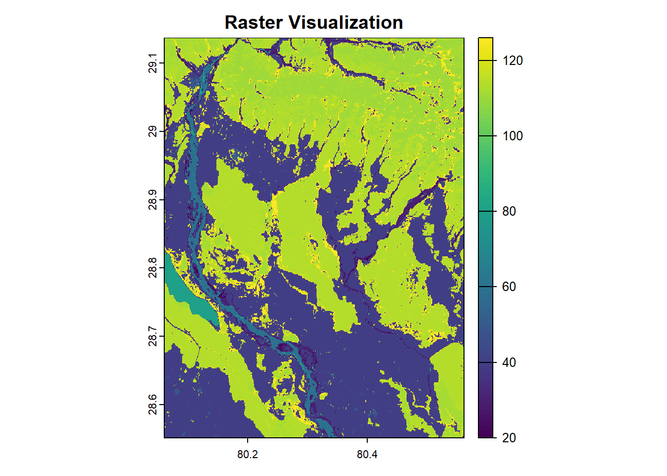
As seen in the plot above, the cell values range from 20 to over 120.
Clipping
Clipping a raster limits its extent to a specific area of interest. It helps reduce file size and ensures analysis is focused on relevant regions. In terra, clipping can be performed using the crop() function, which takes a raster and a bounding box or spatial object to define the extent.
# Import a sf object which you have already downloaded i.e. Sreepur gpkg
library(sf)
spr <-
  read_sf("data/vector/sreepur.gpkg")

# Clip the raster
lc_2015_crop <-
  terra::crop(lc_2015, spr)

# Plot the clipped raster
plot(lc_2015_crop,
     main = "Clipped Raster")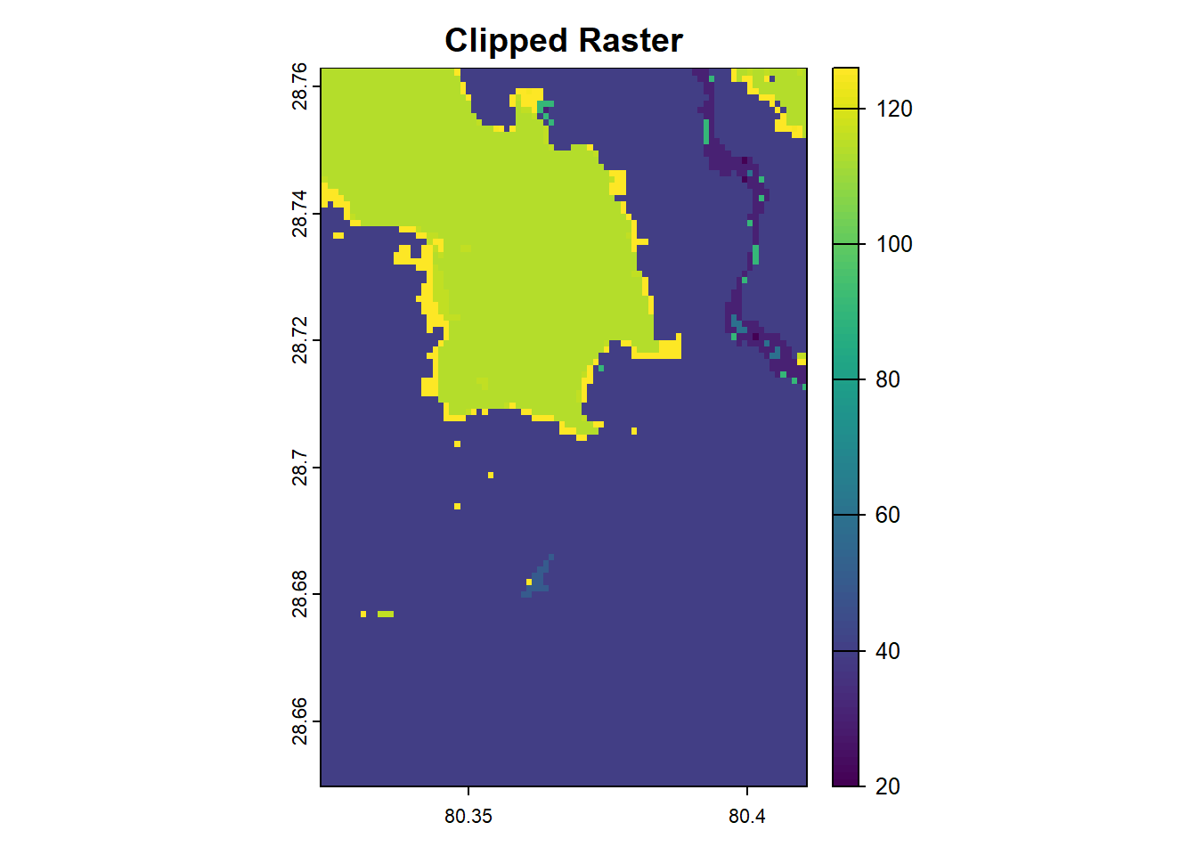
Masking
Masking modifies a raster by setting values outside a specified region to NA. This operation is particularly useful for applying spatial masks, such as land polygons, to exclude unwanted areas like oceans. The mask() function achieves this by combining a raster and a spatial object (e.g., vector polygons).
# Mask the raster
lc_2015_mask <-
  terra::mask(lc_2015_crop,
              spr)

# Plot the clipped raster
plot(lc_2015_mask,
     main = "Masked Raster")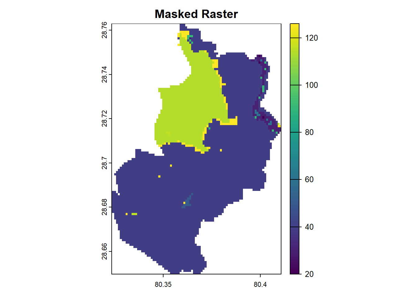
Masking helps refine raster datasets by focusing on specific areas or excluding irrelevant regions.
Reclassification
Reclassification involves categorizing raster cell values into meaningful classes. For example, a raster of population count values can be reclassified into categories such as “Low,” “Medium,” and “High.” And a raster of Land cover values can be reclassified into their original land cover type categories. The classify() function in terra simplifies this process by applying specified rules to the raster.
Before performing reclassification, we need to determine the exact values (min, max) of the raster.
# determine minimum and maximum values from the masked raster
terra::minmax(lc_2015_mask)[1:2, ]
min max
20 126 # determine the unique values in the raster, as each cell value in the land cover data represents a different land cover type
table(unique(values(lc_2015_mask)))
 20  30  40  50  60  90 114 116 124 126
  1   1   1   1   1   1   1   1   1   1
As we can see, there are 10 different values within the masked raster, indicating that there are 10 distinct land cover types within the Sreepur polygon.
The ESA Product User Manual provides essential information on their data products, data values, and corresponding land cover types. For your convenience, I have listed all 23 discrete classes below.
20 - Shrubland, 30 - Grassland, 40 - Cropland, 50 - Built-up, 60 - Bare/Sparse Vegetation, 70 - Snow and Ice, 80 - Permanent Water Bodies, 90 - Herbaceous Wetland, 100 - Moss, 111 - Closed Forest Evergreen Needle Leaf, 112 - Closed Forest Evergreen Broad Leaf, 113 - Closed Forest Deciduous Needle Leaf, 114 - Closed Forest Deciduous Broad Leaf, 115 - Closed Forest Mixed, 116 - Closed Forest Unknown, 121 - Open Forest Evergreen Needle Leaf, 122 - Open Forest Evergreen Broad Leaf, 123 - Open Forest Deciduous Needle Leaf, 124 - Open Forest Deciduous Broad Leaf, 125 - Open Forest Mixed, 126 - Open Forest Unknown, 200 - Open Sea & 0 - Empty
However, for this tutorial and our specific area of ineterst, we will use only the necessary classes and modify them for our convenience.
# Reclassify raster values into new categories
# Define reclassification rules: from-to, new value
rules <- matrix(c(19, 21, 1,
                  29, 31, 2,
                  39, 41, 3,
                  49, 51, 4,
                  59, 61, 5,
                  89, 91, 6,
                  113, 117, 7,
                  123, 127, 8),
                ncol = 3, byrow = TRUE)

# Apply reclassification on masked raster
reclassified_raster <- terra::classify(lc_2015_mask,
                                       rules)

# Convert the numeric raster to a factor (or character) with labels
levels(reclassified_raster) <- data.frame(value = c(1, 2, 3, 4, 5, 6, 7, 8),
                                          label = c("Shrubland", "Grassland", "Cropland", "Built-Up",
                                                    "Sparse Vegetation", "Herbaceous wetland", "Closed Forest", "Open Forest"))

# Plot the reclassified raster
plot(reclassified_raster, main = "Reclassified Raster")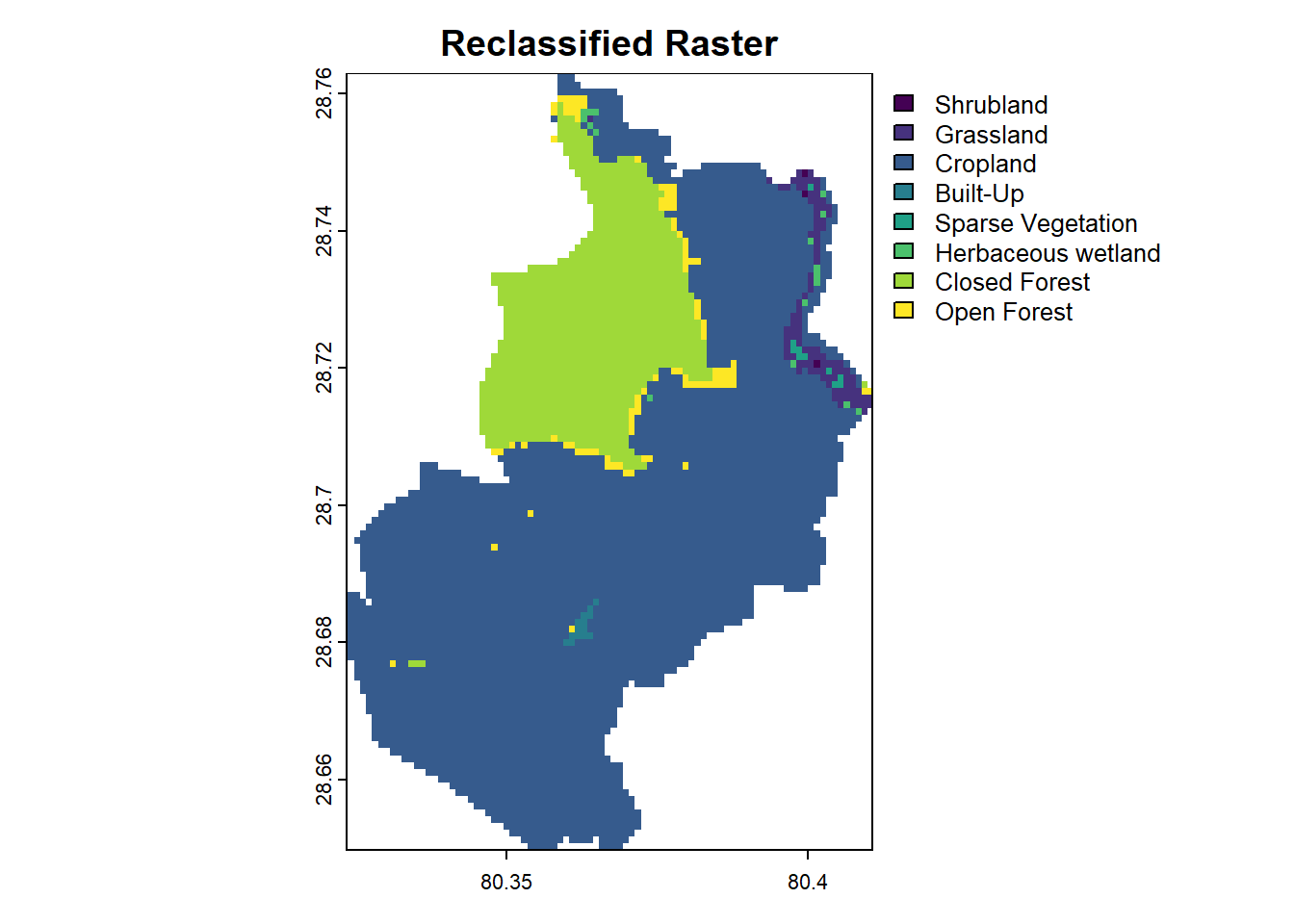
Working with raster data often involves visualizing the dataset, reclassifying values into meaningful categories, and refining spatial coverage through clipping and masking. The terra package provides powerful tools to perform these operations efficiently. These capabilities allow users to tailor raster datasets to their specific analytical needs, enabling effective geospatial analysis.
sessionInfo()R version 4.4.0 (2024-04-24 ucrt)
Platform: x86_64-w64-mingw32/x64
Running under: Windows 11 x64 (build 22631)
Matrix products: default
locale:
[1] LC_COLLATE=English_Germany.utf8 LC_CTYPE=English_Germany.utf8
[3] LC_MONETARY=English_Germany.utf8 LC_NUMERIC=C
[5] LC_TIME=English_Germany.utf8
time zone: Europe/Berlin
tzcode source: internal
attached base packages:
[1] stats graphics grDevices utils datasets methods base
other attached packages:
[1] sf_1.0-19 terra_1.8-5 workflowr_1.7.1
loaded via a namespace (and not attached):
[1] jsonlite_1.8.8 highr_0.11 compiler_4.4.0 promises_1.3.0
[5] Rcpp_1.0.13 stringr_1.5.1 git2r_0.33.0 callr_3.7.6
[9] later_1.3.2 jquerylib_0.1.4 yaml_2.3.10 fastmap_1.2.0
[13] R6_2.5.1 classInt_0.4-10 knitr_1.48 tibble_3.2.1
[17] units_0.8-5 rprojroot_2.0.4 DBI_1.2.3 bslib_0.8.0
[21] pillar_1.9.0 rlang_1.1.4 utf8_1.2.4 cachem_1.1.0
[25] stringi_1.8.4 httpuv_1.6.15 xfun_0.47 getPass_0.2-4
[29] fs_1.6.4 sass_0.4.9 cli_3.6.3 magrittr_2.0.3
[33] class_7.3-22 ps_1.8.1 grid_4.4.0 digest_0.6.36
[37] processx_3.8.4 rstudioapi_0.16.0 lifecycle_1.0.4 vctrs_0.6.5
[41] KernSmooth_2.23-22 proxy_0.4-27 evaluate_0.24.0 glue_1.7.0
[45] whisker_0.4.1 codetools_0.2-20 e1071_1.7-16 fansi_1.0.6
[49] rmarkdown_2.28 httr_1.4.7 tools_4.4.0 pkgconfig_2.0.3
[53] htmltools_0.5.8.1