Data Frames in R

What is a Data Frame?

Creating Data Frames

Accessing and Modifying Data

Data Frame Operations

Geospatial Data Frames

Creating GDF
Manipulating GDF

Last updated: 2025-01-02

Checks: 7 0

Knit directory: R_tutorial/

This reproducible R Markdown analysis was created with workflowr (version 1.7.1). The Checks tab describes the reproducibility checks that were applied when the results were created. The Past versions tab lists the development history.

R Markdown file: up-to-date

Great! Since the R Markdown file has been committed to the Git repository, you know the exact version of the code that produced these results.

Environment: empty

Great job! The global environment was empty. Objects defined in the global environment can affect the analysis in your R Markdown file in unknown ways. For reproduciblity it’s best to always run the code in an empty environment.

Seed: set.seed(20241223)

The command set.seed(20241223) was run prior to running the code in the R Markdown file. Setting a seed ensures that any results that rely on randomness, e.g. subsampling or permutations, are reproducible.

Session information: recorded

Great job! Recording the operating system, R version, and package versions is critical for reproducibility.

Cache: none

Nice! There were no cached chunks for this analysis, so you can be confident that you successfully produced the results during this run.

File paths: relative

Great job! Using relative paths to the files within your workflowr project makes it easier to run your code on other machines.

Repository version: f7832cd

Great! You are using Git for version control. Tracking code development and connecting the code version to the results is critical for reproducibility.

The results in this page were generated with repository version f7832cd. See the Past versions tab to see a history of the changes made to the R Markdown and HTML files.

Note that you need to be careful to ensure that all relevant files for the analysis have been committed to Git prior to generating the results (you can use wflow_publish or wflow_git_commit). workflowr only checks the R Markdown file, but you know if there are other scripts or data files that it depends on. Below is the status of the Git repository when the results were generated:


Ignored files:
    Ignored:    .Rhistory
    Ignored:    .Rproj.user/

Note that any generated files, e.g. HTML, png, CSS, etc., are not included in this status report because it is ok for generated content to have uncommitted changes.

These are the previous versions of the repository in which changes were made to the R Markdown (analysis/Data_Frames.Rmd) and HTML (docs/Data_Frames.html) files. If you’ve configured a remote Git repository (see ?wflow_git_remote), click on the hyperlinks in the table below to view the files as they were in that past version.

File	Version	Author	Date	Message
Rmd	f7832cd	Ohm-Np	2025-01-02	wflow_publish("analysis/Data_Frames.Rmd")
html	d11d577	Ohm-Np	2025-01-01	Build site.
Rmd	1782ac4	Ohm-Np	2025-01-01	wflow_publish("analysis/Data_Frames.Rmd")

What is a Data Frame?

Data frames are a cornerstone of data manipulation and analysis in R, designed for handling tabular data efficiently. They are two-dimensional, rectangular structures where rows represent observations and columns represent variables. Each column is a vector of equal length, allowing for the storage of mixed data types such as numerical, character, or logical values. Analogous to spreadsheets or SQL tables, data frames are indispensable in tasks like statistical analysis, data visualization, and machine learning.

Key characteristics of data frames:

Columns can contain different data types (e.g., numeric, character, factor).
Rows represent individual observations or cases.
Data frames can hold large datasets efficiently.

Creating Data Frames

We can create a data frame in R using the data.frame() function from base R. Here’s an example:

# Creating a data frame
students <- data.frame(
  Name = c("Amrit", "Ishwor", "Indra", "Rakshya"),
  Age = c(27, 24, 21, 25),
  Grade = c("A", "B", "A", "B"),
  Major = c("Maths", "Science", "Maths", "Science")
)

# Display the data frame
print(students)

     Name Age Grade   Major
1   Amrit  27     A   Maths
2  Ishwor  24     B Science
3   Indra  21     A   Maths
4 Rakshya  25     B Science

Accessing and Modifying Data

Selecting Rows and Columns

We can access elements of a data frame using indexing, column names, or logical conditions.

# Access a specific column
students$Name

[1] "Amrit"   "Ishwor"  "Indra"   "Rakshya"

# Access a specific row
students[1, ]

   Name Age Grade Major
1 Amrit  27     A Maths

# Access a specific value
students[2, "Grade"]

[1] "B"

Adding and Removing Columns

We can add a new column to a data frame dynamically or remove an existing column.

# Adding a new column
students$Passed <- c(TRUE, FALSE, TRUE, FALSE)
# Display the data frame
print(students)

     Name Age Grade   Major Passed
1   Amrit  27     A   Maths   TRUE
2  Ishwor  24     B Science  FALSE
3   Indra  21     A   Maths   TRUE
4 Rakshya  25     B Science  FALSE

# Removing a column
students$Grade <- NULL
# Display the data frame
print(students)

     Name Age   Major Passed
1   Amrit  27   Maths   TRUE
2  Ishwor  24 Science  FALSE
3   Indra  21   Maths   TRUE
4 Rakshya  25 Science  FALSE

Data Frame Operations

Filtering and Subsetting

We can filter rows based on conditions using logical operators.

# Filter students with Age > 22
students[students$Age > 22, ]

     Name Age   Major Passed
1   Amrit  27   Maths   TRUE
2  Ishwor  24 Science  FALSE
4 Rakshya  25 Science  FALSE

Sorting and Reordering

Sorting a data frame is straightforward with the order() function.

# Sort by Age
students <- students[order(students$Age), ]
# Display the data frame
print(students)

     Name Age   Major Passed
3   Indra  21   Maths   TRUE
2  Ishwor  24 Science  FALSE
4 Rakshya  25 Science  FALSE
1   Amrit  27   Maths   TRUE

Summary and Statistical Functions

R provides built-in functions to summarize and analyze data frames.

# Summary statistics
summary(students)

     Name                Age           Major             Passed       
 Length:4           Min.   :21.00   Length:4           Mode :logical  
 Class :character   1st Qu.:23.25   Class :character   FALSE:2        
 Mode  :character   Median :24.50   Mode  :character   TRUE :2        
                    Mean   :24.25                                     
                    3rd Qu.:25.50                                     
                    Max.   :27.00

# Number of rows and columns
nrow(students)

[1] 4

ncol(students)

[1] 4

Aggregation and Grouping

The dplyr package functions enable grouping and summarization.

# Load dplyr package
library(dplyr)

# grouping
students %>%
  group_by(Major) %>%
  summarise(Average_Age = mean(Age))

# A tibble: 2 × 2
  Major   Average_Age
  <chr>         <dbl>
1 Maths          24  
2 Science        24.5

So far, this chapter has introduced you to the versatility and power of data frames in R, laying the foundation for data manipulation and analysis. Now, we will delve into data frames specifically designed for geospatial data.

Geospatial Data Frames

A Geospatial Data Frame (GDF) extends a standard data frame by including a geometry column, which stores spatial data in formats such as points, lines, and polygons. This integration of spatial and attribute data makes geospatial data frames ideal for spatial analysis and mapping.

The sf package represents geospatial data frames as sf objects, offering seamless compatibility with other R packages for geospatial and statistical analysis.

Geometry is central to geospatial data frames, defining the spatial features associated with each observation. Each row corresponds to a spatial feature with related attributes, and the geometry column typically stores spatial data in Well-Known Text (WKT) or binary format.

Creating GDF

You can create a geospatial data frame using the st_as_sf() function from the sf package. Here’s an example:

library(sf)

# Create a data frame with spatial data
data <- data.frame(
  Name = c("Point A", "Point B", "Point C"),
  Latitude = c(27.7, 28.2, 26.9),
  Longitude = c(85.3, 84.9, 83.8)
)

# Convert to an sf object
geo_data <- st_as_sf(
  data,
  coords = c("Longitude", "Latitude"),
  crs = 4326  # WGS 84 Coordinate Reference System
)

print(geo_data)

Simple feature collection with 3 features and 1 field
Geometry type: POINT
Dimension:     XY
Bounding box:  xmin: 83.8 ymin: 26.9 xmax: 85.3 ymax: 28.2
Geodetic CRS:  WGS 84
     Name          geometry
1 Point A POINT (85.3 27.7)
2 Point B POINT (84.9 28.2)
3 Point C POINT (83.8 26.9)

Manipulating GDF

Spatial Queries

Geospatial data frames support operations like spatial filtering and proximity analysis.

# Define a bounding box and convert it to an sfc object
bbox <- st_bbox(c(xmin = 84, ymin = 27, xmax = 86, ymax = 29),
                crs = st_crs(geo_data))
bbox_polygon <- 
  st_as_sfc(bbox)

# Filter points within a specific bounding box
filtered_data <- 
  geo_data[st_within(geo_data,
                     bbox_polygon,
                     sparse = FALSE),
           ]

print(filtered_data)

Simple feature collection with 2 features and 1 field
Geometry type: POINT
Dimension:     XY
Bounding box:  xmin: 84.9 ymin: 27.7 xmax: 85.3 ymax: 28.2
Geodetic CRS:  WGS 84
     Name          geometry
1 Point A POINT (85.3 27.7)
2 Point B POINT (84.9 28.2)

Attribute-Based Operations

Just like standard data frames, we can manipulate attributes in geospatial data frames.

# Add a new column
geo_data$Elevation <- 
  c(1500, 2000, 1700)

print(geo_data)

Simple feature collection with 3 features and 2 fields
Geometry type: POINT
Dimension:     XY
Bounding box:  xmin: 83.8 ymin: 26.9 xmax: 85.3 ymax: 28.2
Geodetic CRS:  WGS 84
     Name          geometry Elevation
1 Point A POINT (85.3 27.7)      1500
2 Point B POINT (84.9 28.2)      2000
3 Point C POINT (83.8 26.9)      1700

Visualization of GDF

Geospatial data frames can be visualized using the plot() function from the sf package or integrated with advanced visualization libraries such as ggplot2.

plot(geo_data["Name"],
     main = "Geospatial Data Points")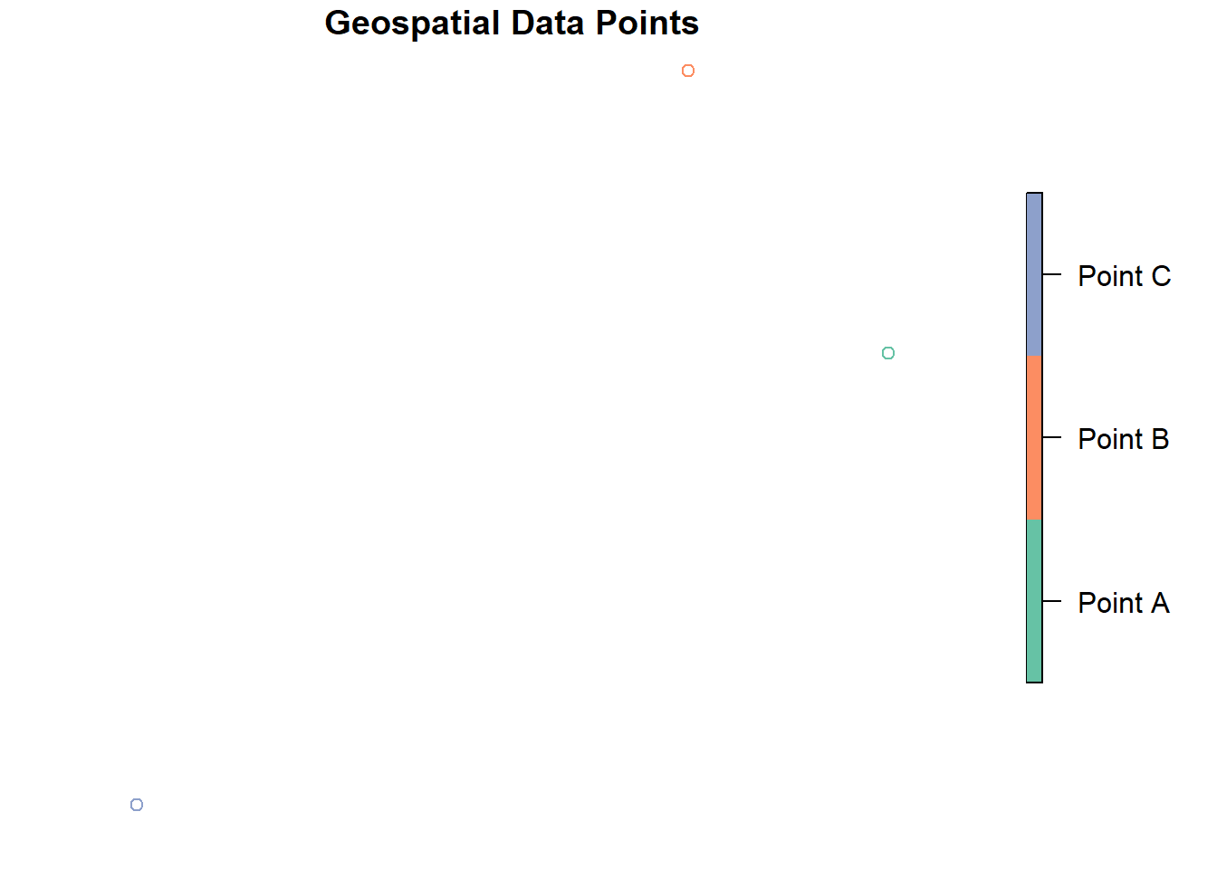

For enhanced visualization, we can use geom_sf() in ggplot2.

library(ggplot2)

ggplot(data = geo_data) +
  geom_sf(aes(color = Name), size = 3) +
  labs(title = "Geospatial Data Points") +
  theme_minimal()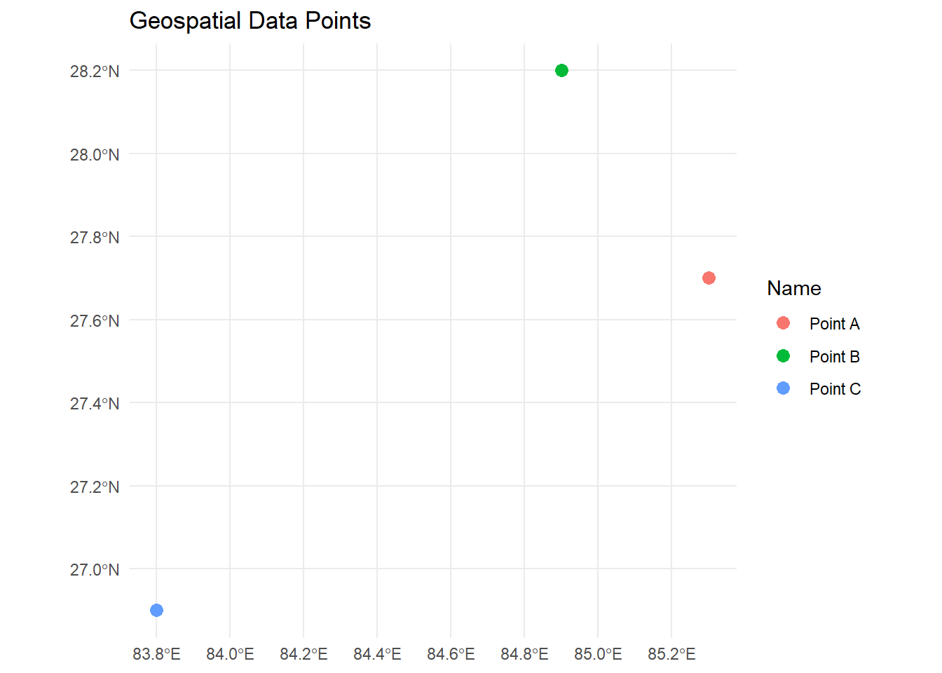

This approach allows you to set individual colors based on the Name attribute or other properties and provides more control over styling.

Geospatial data frames bridge the gap between tabular data and spatial analysis, making them indispensable for modern geospatial workflows. Their versatility, combined with R’s ecosystem of geospatial packages, provides an efficient and intuitive way to analyze and visualize spatial data.

sessionInfo()

R version 4.4.0 (2024-04-24 ucrt)
Platform: x86_64-w64-mingw32/x64
Running under: Windows 11 x64 (build 22631)

Matrix products: default


locale:
[1] LC_COLLATE=English_Germany.utf8  LC_CTYPE=English_Germany.utf8   
[3] LC_MONETARY=English_Germany.utf8 LC_NUMERIC=C                    
[5] LC_TIME=English_Germany.utf8    

time zone: Europe/Berlin
tzcode source: internal

attached base packages:
[1] stats     graphics  grDevices utils     datasets  methods   base     

other attached packages:
[1] ggplot2_3.5.1   sf_1.0-19       dplyr_1.1.4     workflowr_1.7.1

loaded via a namespace (and not attached):
 [1] s2_1.1.7           sass_0.4.9         utf8_1.2.4         generics_0.1.3    
 [5] class_7.3-22       KernSmooth_2.23-22 stringi_1.8.4      digest_0.6.36     
 [9] magrittr_2.0.3     evaluate_0.24.0    grid_4.4.0         fastmap_1.2.0     
[13] rprojroot_2.0.4    jsonlite_1.8.8     processx_3.8.4     whisker_0.4.1     
[17] e1071_1.7-16       DBI_1.2.3          ps_1.8.1           promises_1.3.0    
[21] httr_1.4.7         fansi_1.0.6        scales_1.3.0       jquerylib_0.1.4   
[25] cli_3.6.3          rlang_1.1.4        units_0.8-5        munsell_0.5.1     
[29] withr_3.0.2        cachem_1.1.0       yaml_2.3.10        tools_4.4.0       
[33] colorspace_2.1-1   httpuv_1.6.15      vctrs_0.6.5        R6_2.5.1          
[37] proxy_0.4-27       lifecycle_1.0.4    classInt_0.4-10    git2r_0.33.0      
[41] stringr_1.5.1      fs_1.6.4           pkgconfig_2.0.3    callr_3.7.6       
[45] gtable_0.3.5       pillar_1.9.0       bslib_0.8.0        later_1.3.2       
[49] glue_1.7.0         Rcpp_1.0.13        highr_0.11         xfun_0.47         
[53] tibble_3.2.1       tidyselect_1.2.1   rstudioapi_0.16.0  knitr_1.48        
[57] farver_2.1.2       htmltools_0.5.8.1  rmarkdown_2.28     wk_0.9.4          
[61] compiler_4.4.0     getPass_0.2-4