Integrate and cluster other cells
Jovana Maksimovic and George Howitt
March 20, 2024
Last updated: 2024-03-20
Checks: 7 0
Knit directory: paed-inflammation-CITEseq/
This reproducible R Markdown analysis was created with workflowr (version 1.7.1). The Checks tab describes the reproducibility checks that were applied when the results were created. The Past versions tab lists the development history.
Great! Since the R Markdown file has been committed to the Git repository, you know the exact version of the code that produced these results.
Great job! The global environment was empty. Objects defined in the global environment can affect the analysis in your R Markdown file in unknown ways. For reproduciblity it’s best to always run the code in an empty environment.
The command set.seed(20240216) was run prior to running
the code in the R Markdown file. Setting a seed ensures that any results
that rely on randomness, e.g. subsampling or permutations, are
reproducible.
Great job! Recording the operating system, R version, and package versions is critical for reproducibility.
Nice! There were no cached chunks for this analysis, so you can be confident that you successfully produced the results during this run.
Great job! Using relative paths to the files within your workflowr project makes it easier to run your code on other machines.
Great! You are using Git for version control. Tracking code development and connecting the code version to the results is critical for reproducibility.
The results in this page were generated with repository version 6f4600b. See the Past versions tab to see a history of the changes made to the R Markdown and HTML files.
Note that you need to be careful to ensure that all relevant files for
the analysis have been committed to Git prior to generating the results
(you can use wflow_publish or
wflow_git_commit). workflowr only checks the R Markdown
file, but you know if there are other scripts or data files that it
depends on. Below is the status of the Git repository when the results
were generated:
Ignored files:
    Ignored:    .Rhistory
    Ignored:    .Rproj.user/
    Ignored:    data/C133_Neeland_batch0/
    Ignored:    data/C133_Neeland_batch1/
    Ignored:    data/C133_Neeland_batch2/
    Ignored:    data/C133_Neeland_batch3/
    Ignored:    data/C133_Neeland_batch4/
    Ignored:    data/C133_Neeland_batch5/
    Ignored:    data/C133_Neeland_batch6/
    Ignored:    data/C133_Neeland_merged/
    Ignored:    renv/library/
    Ignored:    renv/staging/

Untracked files:
    Untracked:  analysis/scar.Rmd
    Untracked:  analysis/scar.nb.html
    Untracked:  output/cluster_markers/ADT/
    Untracked:  output/cluster_markers/ADT_decontx/
    Untracked:  output/cluster_markers/RNA/
    Untracked:  output/cluster_markers/RNA_decontx/

Unstaged changes:
    Deleted:    output/cluster_markers/t_cells/REACTOME-cluster-limma-c0.csv
    Deleted:    output/cluster_markers/t_cells/REACTOME-cluster-limma-c1.csv
    Deleted:    output/cluster_markers/t_cells/REACTOME-cluster-limma-c10.csv
    Deleted:    output/cluster_markers/t_cells/REACTOME-cluster-limma-c11.csv
    Deleted:    output/cluster_markers/t_cells/REACTOME-cluster-limma-c12.csv
    Deleted:    output/cluster_markers/t_cells/REACTOME-cluster-limma-c13.csv
    Deleted:    output/cluster_markers/t_cells/REACTOME-cluster-limma-c14.csv
    Deleted:    output/cluster_markers/t_cells/REACTOME-cluster-limma-c15.csv
    Deleted:    output/cluster_markers/t_cells/REACTOME-cluster-limma-c16.csv
    Deleted:    output/cluster_markers/t_cells/REACTOME-cluster-limma-c17.csv
    Deleted:    output/cluster_markers/t_cells/REACTOME-cluster-limma-c18.csv
    Deleted:    output/cluster_markers/t_cells/REACTOME-cluster-limma-c19.csv
    Deleted:    output/cluster_markers/t_cells/REACTOME-cluster-limma-c2.csv
    Deleted:    output/cluster_markers/t_cells/REACTOME-cluster-limma-c20.csv
    Deleted:    output/cluster_markers/t_cells/REACTOME-cluster-limma-c21.csv
    Deleted:    output/cluster_markers/t_cells/REACTOME-cluster-limma-c3.csv
    Deleted:    output/cluster_markers/t_cells/REACTOME-cluster-limma-c4.csv
    Deleted:    output/cluster_markers/t_cells/REACTOME-cluster-limma-c5.csv
    Deleted:    output/cluster_markers/t_cells/REACTOME-cluster-limma-c6.csv
    Deleted:    output/cluster_markers/t_cells/REACTOME-cluster-limma-c7.csv
    Deleted:    output/cluster_markers/t_cells/REACTOME-cluster-limma-c8.csv
    Deleted:    output/cluster_markers/t_cells/REACTOME-cluster-limma-c9.csv
    Deleted:    output/cluster_markers/t_cells/up-cluster-limma-c0.csv
    Deleted:    output/cluster_markers/t_cells/up-cluster-limma-c1.csv
    Deleted:    output/cluster_markers/t_cells/up-cluster-limma-c10.csv
    Deleted:    output/cluster_markers/t_cells/up-cluster-limma-c11.csv
    Deleted:    output/cluster_markers/t_cells/up-cluster-limma-c12.csv
    Deleted:    output/cluster_markers/t_cells/up-cluster-limma-c13.csv
    Deleted:    output/cluster_markers/t_cells/up-cluster-limma-c14.csv
    Deleted:    output/cluster_markers/t_cells/up-cluster-limma-c15.csv
    Deleted:    output/cluster_markers/t_cells/up-cluster-limma-c16.csv
    Deleted:    output/cluster_markers/t_cells/up-cluster-limma-c17.csv
    Deleted:    output/cluster_markers/t_cells/up-cluster-limma-c18.csv
    Deleted:    output/cluster_markers/t_cells/up-cluster-limma-c19.csv
    Deleted:    output/cluster_markers/t_cells/up-cluster-limma-c2.csv
    Deleted:    output/cluster_markers/t_cells/up-cluster-limma-c20.csv
    Deleted:    output/cluster_markers/t_cells/up-cluster-limma-c21.csv
    Deleted:    output/cluster_markers/t_cells/up-cluster-limma-c3.csv
    Deleted:    output/cluster_markers/t_cells/up-cluster-limma-c4.csv
    Deleted:    output/cluster_markers/t_cells/up-cluster-limma-c5.csv
    Deleted:    output/cluster_markers/t_cells/up-cluster-limma-c6.csv
    Deleted:    output/cluster_markers/t_cells/up-cluster-limma-c7.csv
    Deleted:    output/cluster_markers/t_cells/up-cluster-limma-c8.csv
    Deleted:    output/cluster_markers/t_cells/up-cluster-limma-c9.csv
Note that any generated files, e.g. HTML, png, CSS, etc., are not included in this status report because it is ok for generated content to have uncommitted changes.
These are the previous versions of the repository in which changes were
made to the R Markdown
(analysis/08.0_integrate_cluster_other_cells.Rmd) and HTML
(docs/08.0_integrate_cluster_other_cells.html) files. If
you’ve configured a remote Git repository (see
?wflow_git_remote), click on the hyperlinks in the table
below to view the files as they were in that past version.
| File | Version | Author | Date | Message |
|---|---|---|---|---|
| Rmd | 6f4600b | Jovana Maksimovic | 2024-03-20 | wflow_publish(c("analysis/index.Rmd", "analysis/integrate_cluster")) |
Load libraries.
suppressPackageStartupMessages({
 library(SingleCellExperiment)
 library(edgeR)
 library(tidyverse)
 library(ggplot2)
 library(Seurat)
 library(glmGamPoi)
 library(dittoSeq)
 library(here)
 library(clustree)
 library(patchwork)
 library(AnnotationDbi)
 library(org.Hs.eg.db)
 library(glue)
 library(speckle)
 library(tidyHeatmap)
 library(dsb)
})
Load data
Load T-cell subset Seurat object.
ambient <- ""
seu <- readRDS(here("data",
                    "C133_Neeland_merged",
                    glue("C133_Neeland_full_clean{ambient}_other_cells.SEU.rds")))
seu
An object of class Seurat
21894 features across 15687 samples within 3 assays
Active assay: RNA (21568 features, 0 variable features)
2 other assays present: ADT, ADT.dsbData integration
Visualise batch effects.
seu <- ScaleData(seu) %>%
  FindVariableFeatures() %>%
  RunPCA(dims = 1:30, verbose = FALSE) %>%
  RunUMAP(dims = 1:30, verbose = FALSE)

DimPlot(seu, group.by = "Batch", reduction = "umap")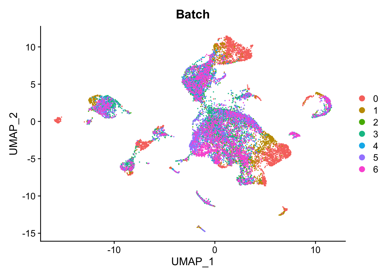
Cell cycle effect
Assign each cell a score, based on its expression of G2/M and S phase markers as described in the Seurat workflow here.
s.genes <- cc.genes.updated.2019$s.genes
g2m.genes <- cc.genes.updated.2019$g2m.genes

seu <- CellCycleScoring(seu, s.features = s.genes, g2m.features = g2m.genes,
                        set.ident = TRUE)
PCA of cell cycle genes.
DimPlot(seu, group.by = "Phase") -> p1

seu %>%
  RunPCA(features = c(s.genes, g2m.genes),
                      dims = 1:30, verbose = FALSE) %>%
  DimPlot(reduction = "pca") -> p2

(p2 / p1) + plot_layout(guides = "collect")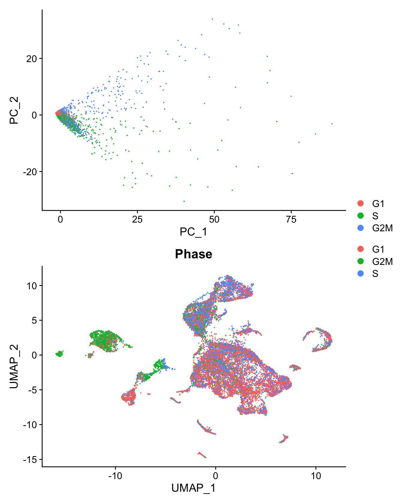
Distribution of cell cycle markers.
# Visualize the distribution of cell cycle markers across
RidgePlot(seu, features = c("PCNA", "TOP2A", "MCM6", "MKI67"), ncol = 2,
          log = TRUE)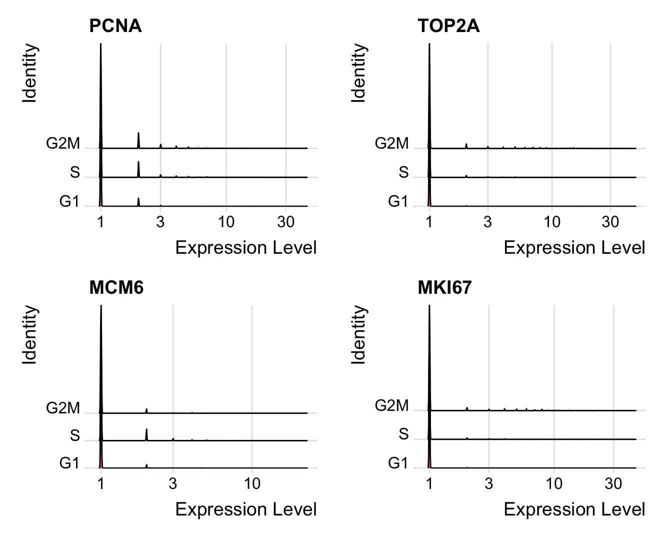
Using the Seurat Alternate Workflow from here,
calculate the difference between the G2M and S phase scores so that
signals separating non-cycling cells and cycling cells will be
maintained, but differences in cell cycle phase among proliferating
cells (which are often uninteresting), can be regressed out of the
data.
seu$CC.Difference <- seu$S.Score - seu$G2M.ScoreIntegrate RNA data
Split by batch for integration. Normalise with
SCTransform. Increase the strength of alignment by
increasing k.anchor parameter to 20 as recommended in
Seurat Fast integration with RPCA vignette.
First, integrate the RNA data.
out <- here("data",
            "C133_Neeland_merged",
            glue("C133_Neeland_full_clean{ambient}_integrated_other_cells.SEU.rds"))

if(!file.exists(out)){
  DefaultAssay(seu) <- "RNA"
  VariableFeatures(seu) <- NULL
  seu[["pca"]] <- NULL
  seu[["umap"]] <- NULL

  seuLst <- SplitObject(seu, split.by = "Batch")
  rm(seu)
  gc()

  # normalise with SCTransform and regress out cell cycle score difference
  seuLst <- lapply(X = seuLst, FUN = SCTransform, method = "glmGamPoi",
                   vars.to.regress = "CC.Difference")
  # integrate RNA data
  features <- SelectIntegrationFeatures(object.list = seuLst,
                                        nfeatures = 3000)
  seuLst <- PrepSCTIntegration(object.list = seuLst, anchor.features = features)
  seuLst <- lapply(X = seuLst, FUN = RunPCA, features = features)
  anchors <- FindIntegrationAnchors(object.list = seuLst,
                                    normalization.method = "SCT",
                                    anchor.features = features,
                                    k.anchor = 20,
                                    dims = 1:30, reduction = "rpca")
  seu <- IntegrateData(anchorset = anchors,
                       k.weight = min(100, min(sapply(seuLst, ncol)) - 5),
                       normalization.method = "SCT",
                       dims = 1:30)

  DefaultAssay(seu) <- "integrated"
  seu <- RunPCA(seu, dims = 1:30, verbose = FALSE) %>%
    RunUMAP(dims = 1:30, verbose = FALSE)

  saveRDS(seu, file = out)
  fs::file_chmod(out, "664")
  if(any(str_detect(fs::group_ids()$group_name,
                    "oshlack_lab"))) fs::file_chown(out,
                                                    group_id = "oshlack_lab")

} else {
  seu <- readRDS(file = out)

}
Integrate ADT data
out <- here("data",
            "C133_Neeland_merged",
            glue("C133_Neeland_full_clean{ambient}_integrated_other_cells.ADT.SEU.rds"))

# get ADT meta data
read.csv(file = here("data",
                     "C133_Neeland_batch1",
                     "data",
                     "sample_sheets",
                     "ADT_features.csv")) -> adt_data
# cleanup ADT meta data
pattern <- "anti-human/mouse |anti-human/mouse/rat |anti-mouse/human "
adt_data$name <- gsub(pattern, "", adt_data$name)
# change ADT rownames to antibody names
DefaultAssay(seu) <- "ADT"
if(all(rownames(seu[["ADT"]]@counts) == adt_data$id)){
  adt_counts <- seu[["ADT"]]@counts
  rownames(adt_counts) <- adt_data$name
  seu[["ADT"]] <- CreateAssayObject(counts = adt_counts)
}

if(!file.exists(out)){
  tmp <- DietSeurat(subset(seu, cells = which(seu$Batch != 0)),
                    assays = "ADT")
  DefaultAssay(tmp) <- "ADT"

  seuLst <- SplitObject(tmp, split.by = "Batch")
  seuLst <- lapply(X = seuLst, FUN = function(x) {
    # set all ADT as variable features
    VariableFeatures(x) <- rownames(x)
    x <- NormalizeData(x, normalization.method = "CLR", margin = 2)
    x
  })
  features <- SelectIntegrationFeatures(object.list = seuLst)
  seuLst <- lapply(X = seuLst, FUN = function(x) {
    x <- ScaleData(x, features = features, verbose = FALSE) %>%
      RunPCA(features = features, verbose = FALSE)
    x
  })
  anchors <- FindIntegrationAnchors(object.list = seuLst, reduction = "rpca",
                                    dims = 1:30)
  tmp <- IntegrateData(anchorset = anchors, dims = 1:30)

  DefaultAssay(tmp) <- "integrated"
  tmp <- ScaleData(tmp) %>%
    RunPCA(dims = 1:30, verbose = FALSE) %>%
    RunUMAP(dims = 1:30, verbose = FALSE)

  # create combined object that only contains cells with RNA+ADT data
  seuADT <- subset(seu, cells = which(seu$Batch !=0))
  seuADT[["integrated.adt"]] <- tmp[["integrated"]]
  seuADT[["pca.adt"]] <- tmp[["pca"]]
  seuADT[["umap.adt"]] <- tmp[["umap"]]

  saveRDS(seuADT, file = out)
  fs::file_chmod(out, "664")
  if(any(str_detect(fs::group_ids()$group_name,
                    "oshlack_lab"))) fs::file_chown(out,
                                                    group_id = "oshlack_lab")

} else {
  seuADT <- readRDS(file = out)

}
View integrated data
DefaultAssay(seuADT) <- "integrated"

DimPlot(seu, group.by = "Batch", reduction = "umap") -> p1
DimPlot(seuADT, group.by = "Batch", reduction = "umap") -> p2
DimPlot(seuADT, group.by = "Batch", reduction = "umap.adt") -> p3

(p1 / ((p2 | p3) +
  plot_layout(guides = "collect"))) &
  theme(axis.title = element_text(size = 8),
axis.text = element_text(size = 8)) 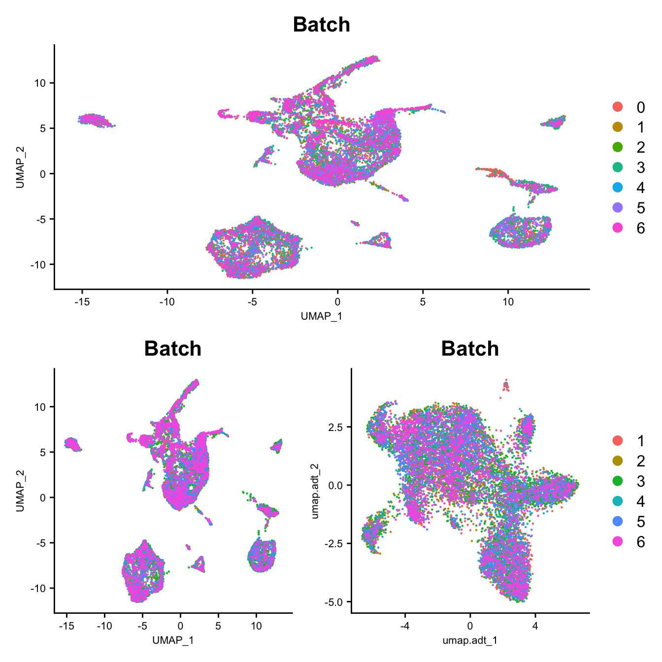
DimPlot(seu, group.by = "Phase", reduction = "umap") -> p1
DimPlot(seuADT, group.by = "Phase", reduction = "umap") -> p2
DimPlot(seuADT, group.by = "Phase", reduction = "umap.adt") -> p3

(p1 / ((p2 | p3) +
  plot_layout(guides = "collect"))) &
  theme(axis.title = element_text(size = 8),
axis.text = element_text(size = 8)) 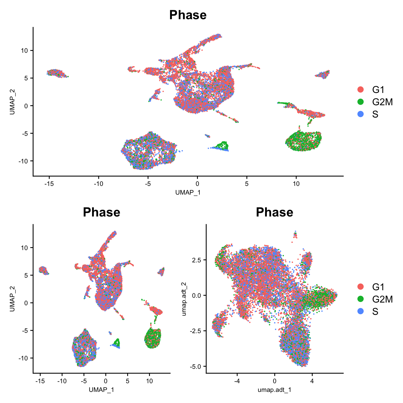
Cluster data
Perform clustering only on data that has ADT i.e. exclude batch 0.
Dimensionality reduction (RNA)
Exclude any mitochondrial, ribosomal, immunoglobulin and HLA genes from variable genes list, to encourage clustering by cell type.
# remove HLA, immunoglobulin, RNA, MT, and RP genes from variable genes list
var_regex = '^HLA-|^IG[HJKL]|^RNA|^MT-|^RP'
hvg <- grep(var_regex, VariableFeatures(seuADT), invert = TRUE, value = TRUE)
# assign edited variable gene list back to object
VariableFeatures(seuADT) <- hvg

# redo PCA and UMAP
seuADT <- RunPCA(seuADT, dims = 1:30, verbose = FALSE) %>%
    RunUMAP(dims = 1:30, verbose = FALSE)

DimHeatmap(seuADT, dims = 1:30, cells = 500, balanced = TRUE,
           reduction = "pca", assays = "integrated")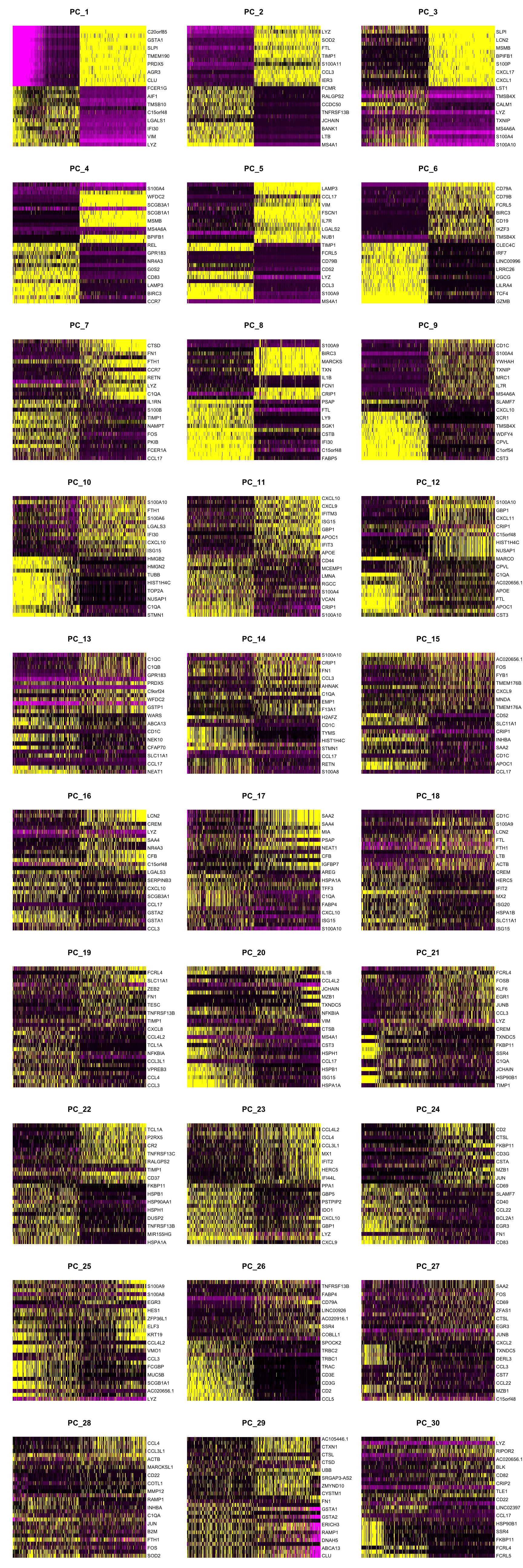
ElbowPlot(seuADT, ndims = 30, reduction = "pca")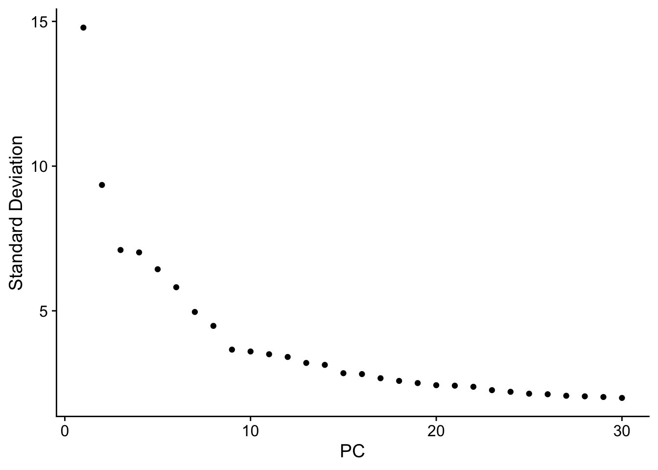
Dimensionality reduction (ADT)
DimHeatmap(seuADT, dims = 1:30, cells = 500, balanced = TRUE,
           reduction = "pca.adt", assays = "integrated.adt")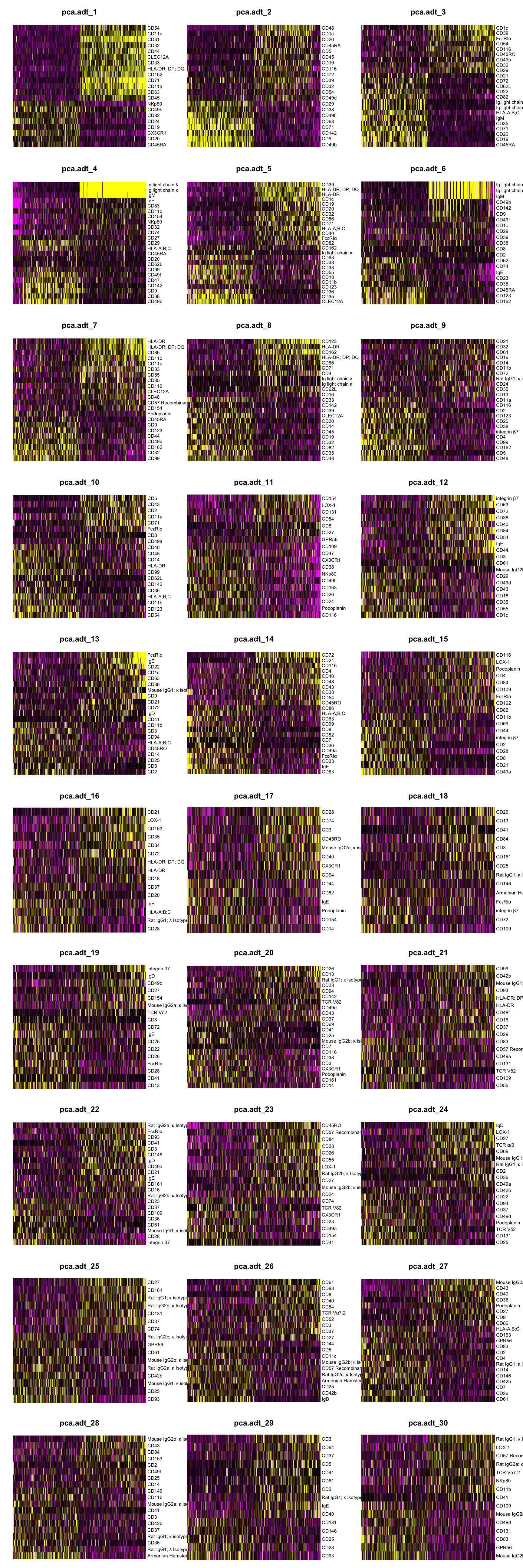
ElbowPlot(seuADT, ndims = 30, reduction = "pca.adt")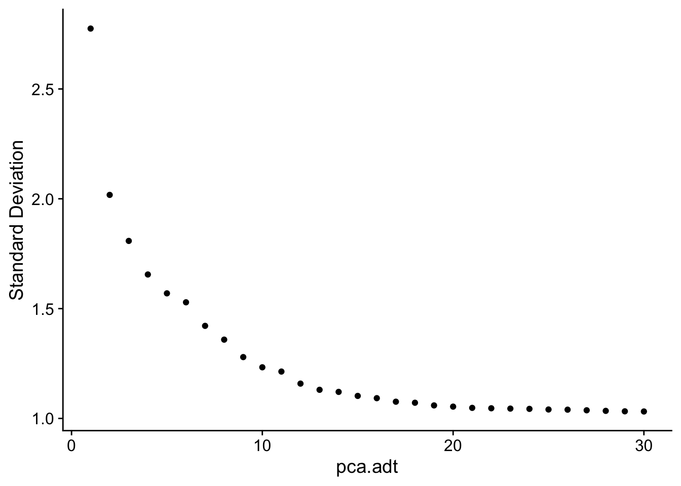
Run WNN clustering
Perform clustering at a range of resolutions and visualise to see which is appropriate to proceed with.
out <- here("data",
            "C133_Neeland_merged",
            glue("C133_Neeland_full_clean{ambient}_integrated_clustered_other_cells.ADT.SEU.rds"))

if(!file.exists(out)){
  DefaultAssay(seuADT) <- "integrated"
  seuADT <- FindMultiModalNeighbors(seuADT, reduction.list = list("pca", "pca.adt"),
                                 dims.list = list(1:30, 1:10),
                                 modality.weight.name = "RNA.weight")
  seuADT <- FindClusters(seuADT, algorithm = 3,
                      resolution = seq(0.1, 1, by = 0.1),
                      graph.name = "wsnn")
  seuADT <- RunUMAP(seuADT, dims = 1:30, nn.name = "weighted.nn",
                 reduction.name = "wnn.umap", reduction.key = "wnnUMAP_",
                 return.model = TRUE)
  saveRDS(seuADT, file = out)
  fs::file_chmod(out, "664")
  if(any(str_detect(fs::group_ids()$group_name,
                    "oshlack_lab"))) fs::file_chown(out,
                                                    group_id = "oshlack_lab")

} else {
  seuADT <- readRDS(file = out)

}

clustree::clustree(seuADT, prefix = "wsnn_res.")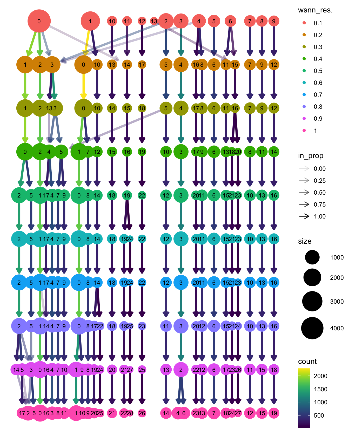
View clusters
Choose most appropriate resolution based on clustree
plot above.
grp <- "wsnn_res.0.6"
# change factor ordering
seuADT@meta.data[,grp] <- fct_inseq(seuADT@meta.data[,grp])

DimPlot(seuADT, group.by = grp, label = T) +
  theme(legend.position = "bottom")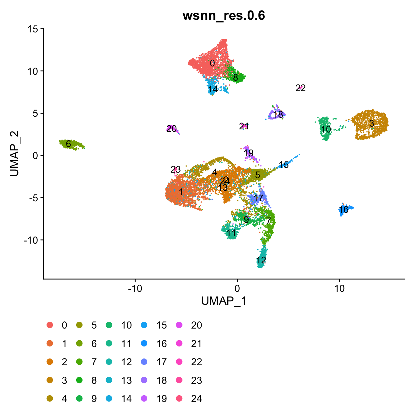
Weighting of RNA and ADT data per cluster.
 VlnPlot(seuADT, features = "integrated.weight", group.by = grp, sort = TRUE,
         pt.size = 0.1) +
  NoLegend()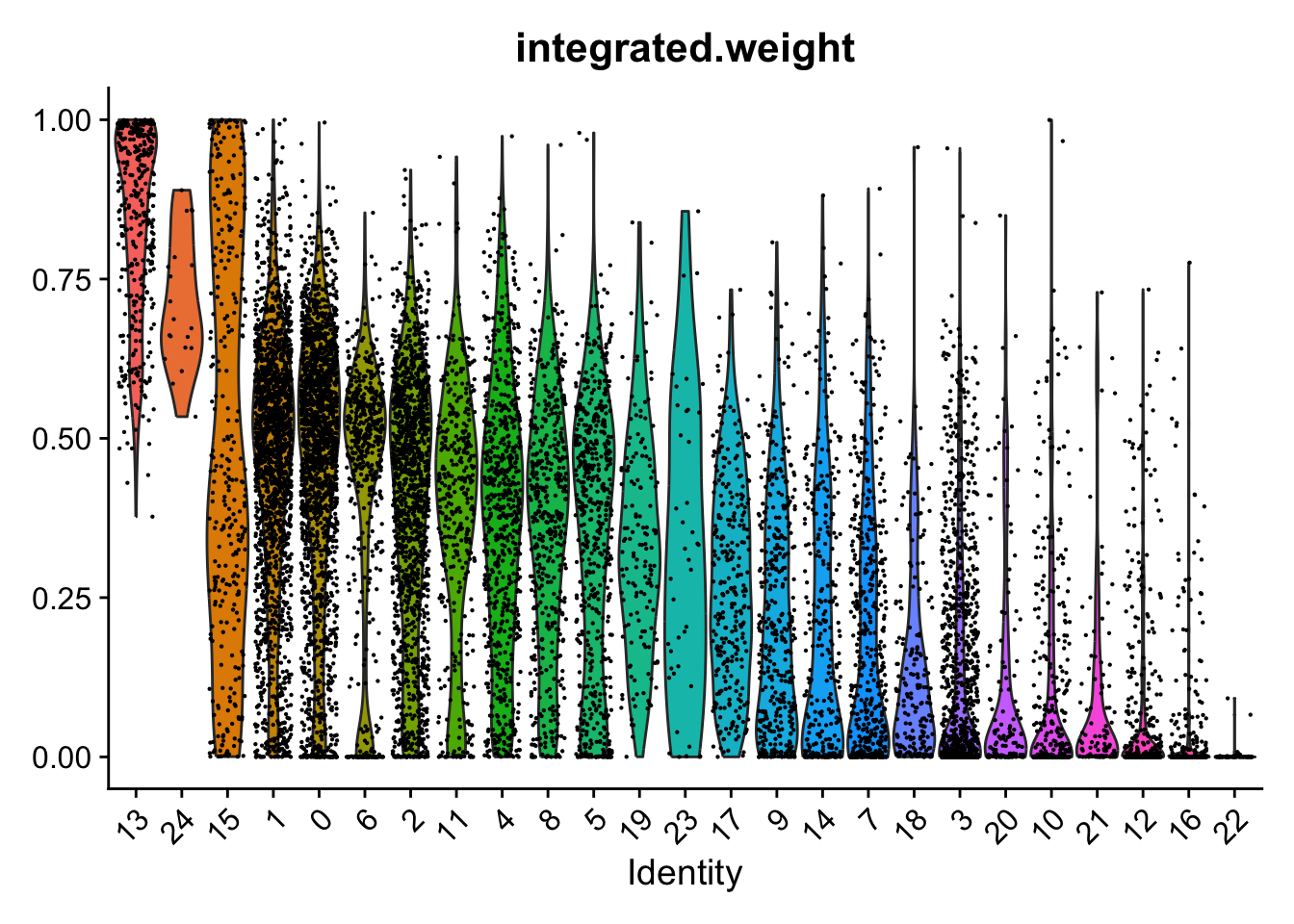
Reference mapping
Batch 0 only has RNA data and was not included in the WNN clustering of batched 1-6. To add this data we will map it to the WNN clustered reference.
Map data
Find transfer anchors.
# use WNN clustered batches 1-6 as reference
reference <- seuADT
DefaultAssay(seu) <- "RNA"
# batch 0 RNA data is the query
query <- DietSeurat(subset(seu, cells = which(seu$Batch == 0)),
                    assays = "RNA")

DefaultAssay(reference) <- "integrated"

anchors <- FindTransferAnchors(
  reference = reference,
  query = query,
  normalization.method = "SCT",
  reference.reduction = "pca",
  dims = 1:50
)
Map batch 0 samples onto reference.
query <- MapQuery(
  anchorset = anchors,
  query = query,
  reference = reference,
  refdata = list(
    wsnn = grp,
    ADT = "ADT"
  ),
  reference.reduction = "pca",
  reduction.model = "wnn.umap"
)

query
An object of class Seurat
21756 features across 2971 samples within 3 assays
Active assay: RNA (21568 features, 0 variable features)
2 other assays present: prediction.score.wsnn, ADT
2 dimensional reductions calculated: ref.pca, ref.umapVisualise batch 0 samples on reference UMAP.
query$predicted.wsnn <- fct_inseq(query$predicted.wsnn)

DimPlot(query, reduction = "ref.umap", group.by = "predicted.wsnn",
        label = TRUE, label.size = 3 ,repel = TRUE) +
  theme(legend.position = "bottom")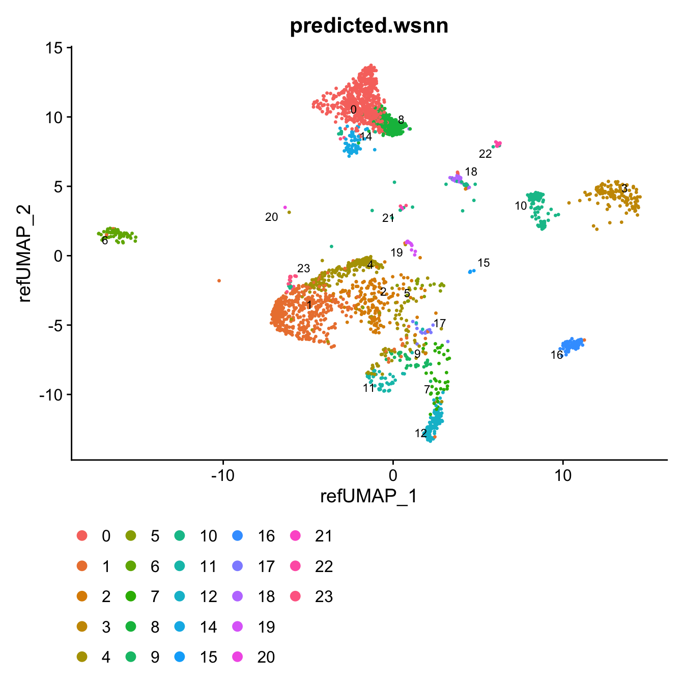
Distribution of Azimuth prediction scores per WNN
cluster.
ggplot(query@meta.data, aes(x = predicted.wsnn,
                            y = predicted.wsnn.score,
                            fill = predicted.wsnn)) +
  geom_boxplot() + NoLegend()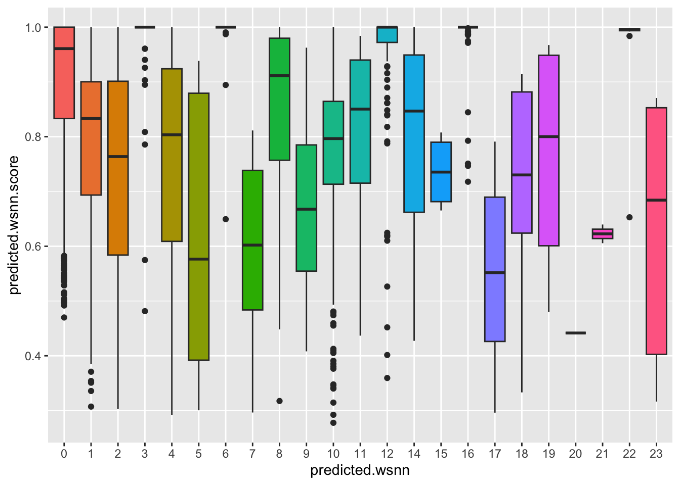
Compute combined UMAP
Computing a new UMAP can help to identify any cell states present in the query but not reference.
# merge reference (integrated + WNN clustered) and query (RNA only samples)
reference$id <- 'reference'
query$id <- 'query'
DefaultAssay(reference) <- "integrated"
refquery <- merge(DietSeurat(reference,
                             assays = c("RNA","ADT","integrated","SCT"),
                             dimreducs = c("pca")),
                  DietSeurat(query,
                             assays = c("RNA"),
                             dimreducs = "ref.pca"))
refquery[["pca"]] <- merge(reference[["pca"]], query[["ref.pca"]])
refquery <- RunUMAP(refquery, reduction = 'pca', dims = 1:50, assay = "integrated")
View combined UMAP.
# combine cluster annotations from reference and query
refquery@meta.data[, grp] <- ifelse(is.na(refquery@meta.data[,grp]),
                          refquery$predicted.wsnn,
                          refquery@meta.data[,grp])
# change factor ordering
refquery@meta.data[,grp] <- fct_inseq(refquery@meta.data[,grp])

DimPlot(refquery, reduction = "umap", group.by = grp,
label = TRUE, label.size = 3) + NoLegend() 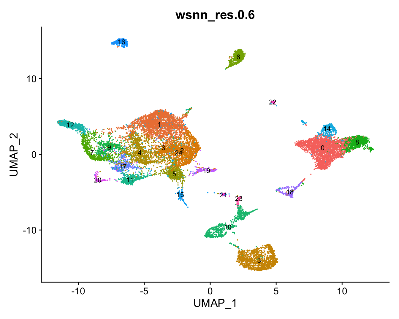
DimPlot(refquery, reduction = "umap", group.by = "Phase",
             label = FALSE, label.size = 3)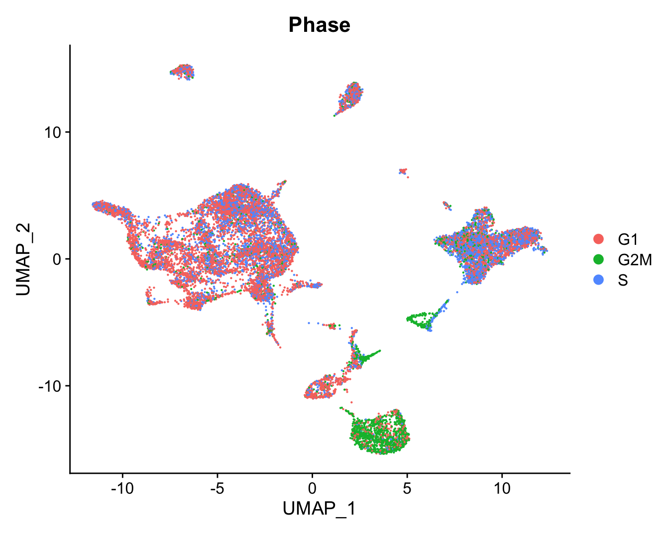
DimPlot(refquery, reduction = "umap", group.by = "Disease",
             label = FALSE, label.size = 3)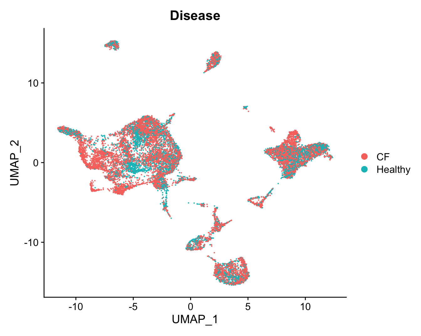
Save results.
out <- here("data",
            "C133_Neeland_merged",
            glue("C133_Neeland_full_clean{ambient}_integrated_clustered_mapped_other_cells.ADT.SEU.rds"))
if(!file.exists(out)){
  saveRDS(refquery, file = out)
  fs::file_chmod(out, "664")
  if(any(str_detect(fs::group_ids()$group_name,
                    "oshlack_lab"))) fs::file_chown(out,
                                                    group_id = "oshlack_lab")
}
Examine combined clusters
Number of cells per cluster.
refquery@meta.data %>%
  ggplot(aes(x = !!sym(grp), fill = !!sym(grp))) +
  geom_bar() +
  geom_text(aes(label = ..count..), stat = "count",
            vjust = -0.5, colour = "black", size = 2) +
  theme(axis.text.x = element_text(angle = 90, vjust = 0.5, hjust = 1)) +
  NoLegend()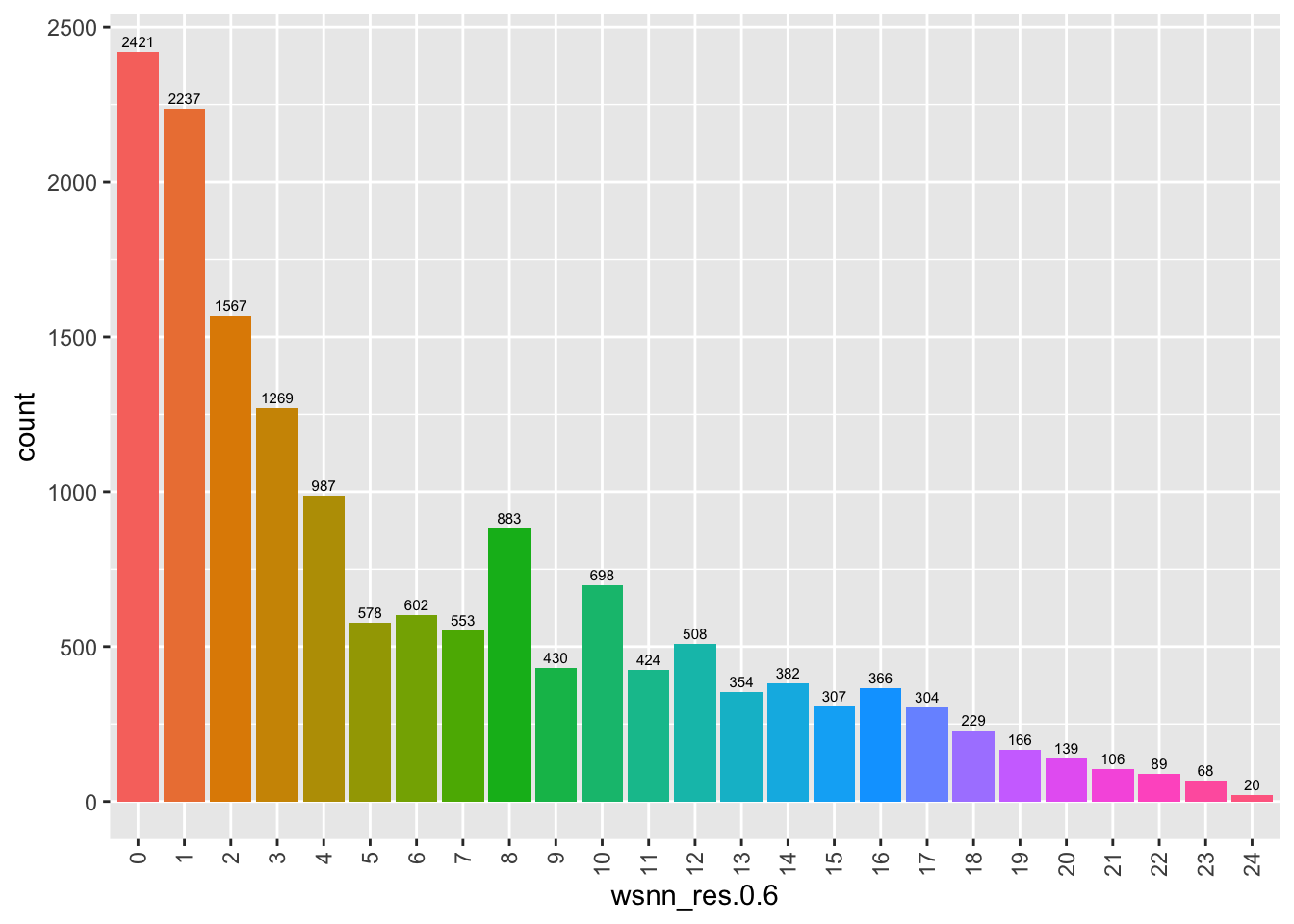
Visualise quality metrics by cluster. Cluster 17 potentially contains low quality cells.
refquery@meta.data %>%
  ggplot(aes(x = !!sym(grp),
             y = nCount_RNA,
             fill = !!sym(grp))) +
  geom_violin(scale = "area") +
  scale_y_log10() +
  NoLegend() -> p2

refquery@meta.data %>%
  ggplot(aes(x = !!sym(grp),
             y = nFeature_RNA,
             fill = !!sym(grp))) +
  geom_violin(scale = "area") +
  scale_y_log10() +
  NoLegend() -> p3

(p2 / p3) & theme(text = element_text(size = 8))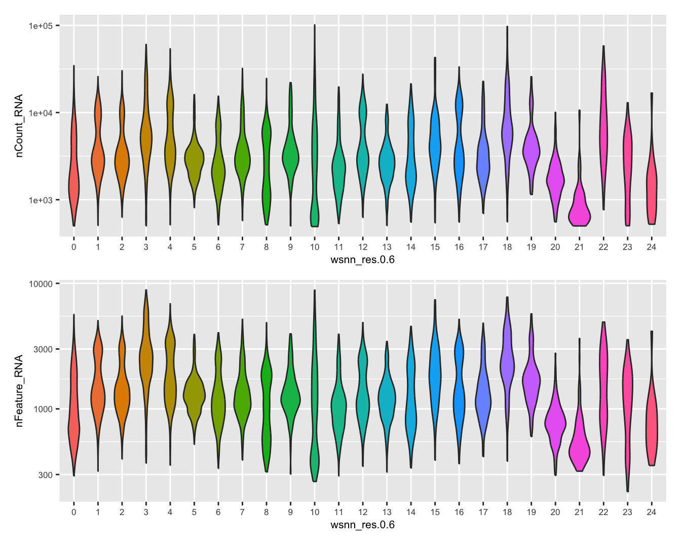
Check the batch composition of each of the clusters. Cluster 17 does not contain any cells from batch 0; could be a quality issue or the cell type was not captured in batch 0?
dittoBarPlot(refquery,
             var = "Batch",
             group.by = grp)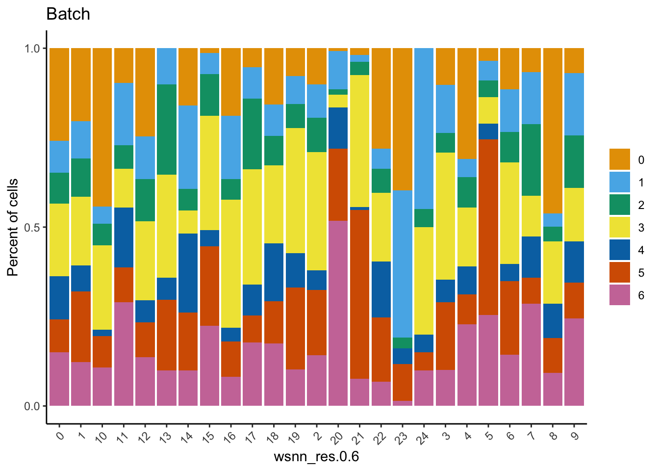
Check the sample compositions of combined clusters.
dittoBarPlot(refquery,
             var = "sample.id",
             group.by = grp) + ggtitle("Samples") +
  theme(legend.position = "bottom")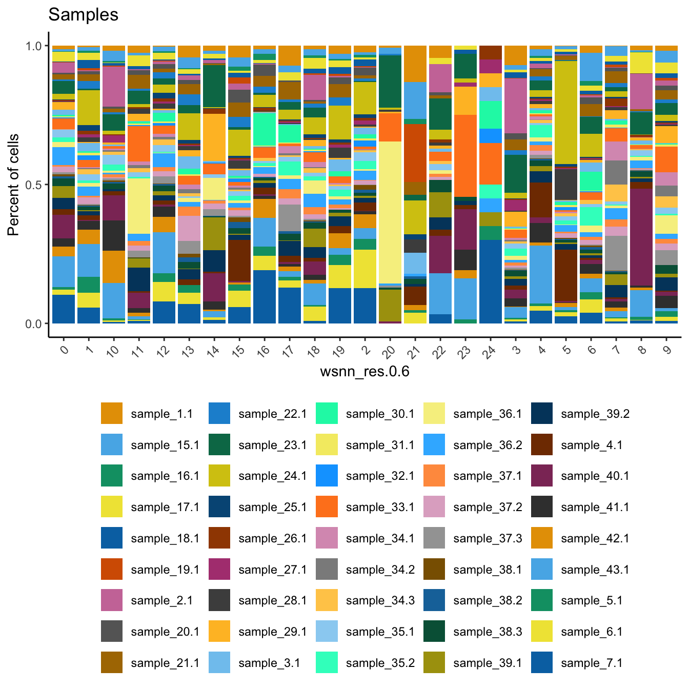
RNA marker gene analysis
Adapted from Dr. Belinda Phipson’s work for [@Sim2021-cg].
Test for marker genes using limma
# limma-trend for DE
Idents(refquery) <- grp

logcounts <- normCounts(DGEList(as.matrix(refquery[["RNA"]]@counts)),
                        log = TRUE, prior.count = 0.5)
entrez <- AnnotationDbi::mapIds(org.Hs.eg.db,
                                keys = rownames(logcounts),
                                column = c("ENTREZID"),
                                keytype = "SYMBOL",
                                multiVals = "first")
# remove genes without entrez IDs as these are difficult to interpret biologically
logcounts <- logcounts[!is.na(entrez),]
# remove confounding genes from counts table e.g. mitochondrial, ribosomal etc.
logcounts <- logcounts[!str_detect(rownames(logcounts), var_regex),]

maxclust <- length(levels(Idents(refquery))) - 1

clustgrp <- paste0("c", Idents(refquery))
clustgrp <- factor(clustgrp, levels = paste0("c", 0:maxclust))
donor <- factor(seu$sample.id)
batch <- factor(seu$Batch)

design <- model.matrix(~ 0 + clustgrp + donor)
colnames(design)[1:(length(levels(clustgrp)))] <- levels(clustgrp)

# Create contrast matrix
mycont <- matrix(NA, ncol = length(levels(clustgrp)),
                 nrow = length(levels(clustgrp)))
rownames(mycont) <- colnames(mycont) <- levels(clustgrp)
diag(mycont) <- 1
mycont[upper.tri(mycont)] <- -1/(length(levels(factor(clustgrp))) - 1)
mycont[lower.tri(mycont)] <- -1/(length(levels(factor(clustgrp))) - 1)

# Fill out remaining rows with 0s
zero.rows <- matrix(0, ncol = length(levels(clustgrp)),
                    nrow = (ncol(design) - length(levels(clustgrp))))
fullcont <- rbind(mycont, zero.rows)
rownames(fullcont) <- colnames(design)

fit <- lmFit(logcounts, design)

fit.cont <- contrasts.fit(fit, contrasts = fullcont)
fit.cont <- eBayes(fit.cont, trend = TRUE, robust = TRUE)

summary(decideTests(fit.cont))
c0 c1 c2 c3 c4 c5 c6 c7 c8 c9 c10 c11
Down 6874 4155 3298 3238 2194 2356 3390 3423 5682 2839 4730 4258
NotSig 7386 9168 9606 4741 11216 11925 10069 11282 8564 12131 8399 10730
Up 2005 2942 3361 8286 2855 1984 2806 1560 2019 1295 3136 1277
c12 c13 c14 c15 c16 c17 c18 c19 c20 c21 c22 c23
Down 4945 738 3325 269 2578 1136 471 216 2748 1687 1109 1140
NotSig 9648 14659 11223 12291 12217 13652 11704 14395 12687 12882 14517 14016
Up 1672 868 1717 3705 1470 1477 4090 1654 830 1696 639 1109
c24
Down 17
NotSig 16078
Up 170Test relative to a threshold (TREAT).
tr <- treat(fit.cont, lfc = 0.25)
dt <- decideTests(tr)
summary(dt)
c0 c1 c2 c3 c4 c5 c6 c7 c8 c9 c10 c11
Down 424 64 38 470 13 45 250 56 535 14 600 83
NotSig 15666 15886 15858 13894 15941 15909 15637 15891 15518 15983 15349 15896
Up 175 315 369 1901 311 311 378 318 212 268 316 286
c12 c13 c14 c15 c16 c17 c18 c19 c20 c21 c22 c23
Down 255 4 264 3 135 9 22 5 131 406 229 176
NotSig 15588 16160 15828 15966 15869 15911 15653 16110 15913 15662 15895 15885
Up 422 101 173 296 261 345 590 150 221 197 141 204
c24
Down 0
NotSig 16263
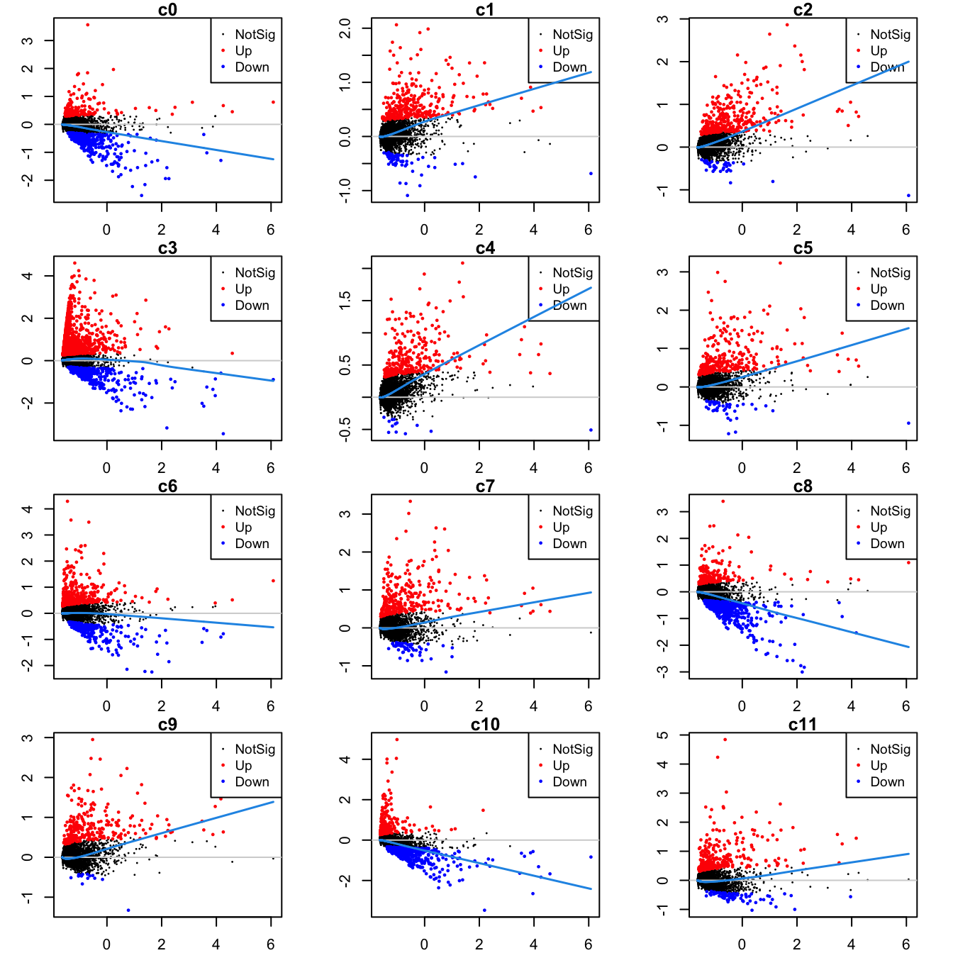
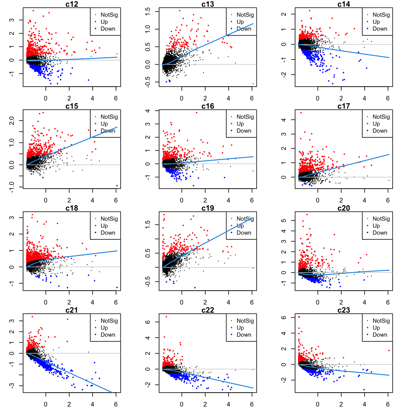
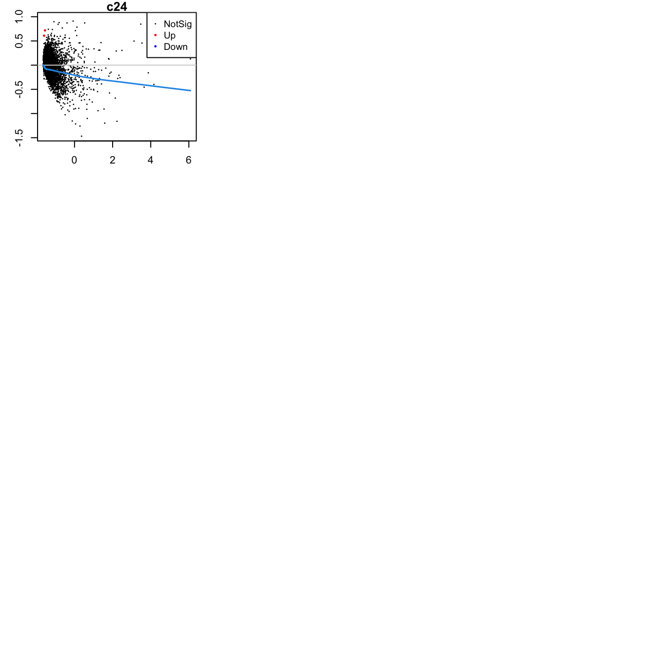
Up 2Mean-difference (MD) plots per cluster.
par(mfrow=c(4,3))
par(mar=c(2,3,1,2))

for(i in 1:ncol(mycont)){
  plotMD(tr, coef = i, status = dt[,i], hl.cex = 0.5)
  abline(h = 0, col = "lightgrey")
  lines(lowess(tr$Amean, tr$coefficients[,i]), lwd = 1.5, col = 4)
}
limma marker gene dotplot
DefaultAssay(refquery) <- "RNA"
contnames <- colnames(mycont)
top_markers <- NULL
n_markers <- 10

for(i in 1:ncol(mycont)){
  top <- topTreat(tr, coef = i, n = Inf)
  top <- top[top$logFC > 0, ]
  top_markers <- c(top_markers,
                   setNames(rownames(top)[1:n_markers],
                            rep(contnames[i], n_markers)))
}

top_markers <- top_markers[!is.na(top_markers)]
top_markers <- top_markers[!duplicated(top_markers)]
cols <- paletteer::paletteer_d("pals::glasbey")[factor(names(top_markers))]

DotPlot(refquery,
        features = unname(top_markers),
        group.by = grp,
        cols = c("azure1", "blueviolet"),
        dot.scale = 3, assay = "SCT") +
    RotatedAxis() +
    FontSize(y.text = 8, x.text = 12) +
    labs(y = element_blank(), x = element_blank()) +
    coord_flip() +
  theme(axis.text.y = element_text(color = cols)) +
  ggtitle("Top 10 cluster marker genes (no duplicates)")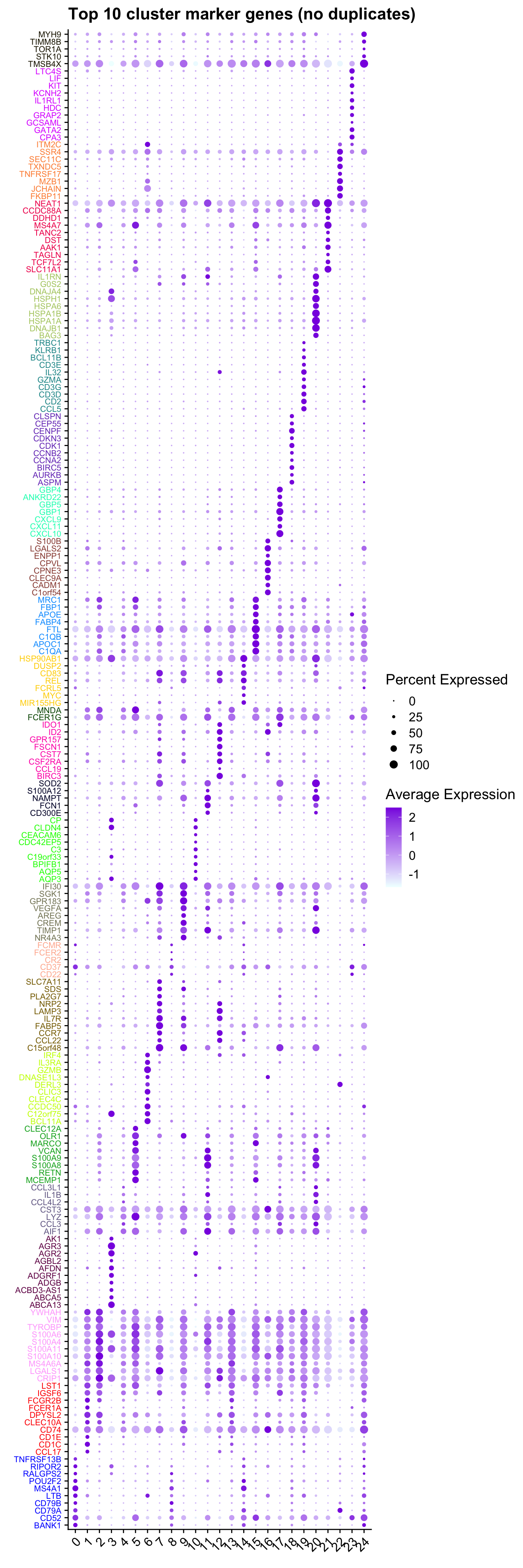
Save marker genes and pathways
The Broad MSigDB Reactome pathways are tested for each contrast using
cameraPR from limma. The cameraPR
method tests whether a set of genes is highly ranked relative to other
genes in terms of differential expression, accounting for inter-gene
correlation.
Prepare gene sets of interest.
if(!file.exists(here("data/Hs.c2.cp.reactome.v7.1.entrez.rds")))
  download.file("https://bioinf.wehi.edu.au/MSigDB/v7.1/Hs.c2.cp.reactome.v7.1.entrez.rds",
                here("data/Hs.c2.cp.reactome.v7.1.entrez.rds"))

Hs.c2.reactome <- readRDS(here("data/Hs.c2.cp.reactome.v7.1.entrez.rds"))

gns <- AnnotationDbi::mapIds(org.Hs.eg.db,
                             keys = rownames(tr),
                             column = c("ENTREZID"),
                             keytype = "SYMBOL",
                             multiVals = "first")
Run pathway analysis and save results to file.
options(scipen=-1, digits = 6)
contnames <- colnames(mycont)
dirName <- here("output",
                "cluster_markers",
                glue("RNA{ambient}"),
                "other_cells")

if(!dir.exists(dirName)) dir.create(dirName, recursive = TRUE)

for(c in colnames(tr)){
  top <- topTreat(tr, coef = c, n = Inf)
  top <- top[top$logFC > 0, ]

  write.csv(top[1:100, ] %>%
              rownames_to_column(var = "Symbol"),
            file = glue("{dirName}/up-cluster-limma-{c}.csv"),
            sep = ",",
            quote = FALSE,
            col.names = NA,
            row.names = TRUE)

  # get marker indices
  c2.id <- ids2indices(Hs.c2.reactome, unname(gns[rownames(tr)]))
  # gene set testing results
  cameraPR(tr$t[,glue("{c}")], c2.id) %>%
    rownames_to_column(var = "Pathway") %>%
    dplyr::filter(Direction == "Up") %>%
    slice_head(n = 50) %>%
    write.csv(file = here(glue("{dirName}/REACTOME-cluster-limma-{c}.csv")),
            sep = ",",
            quote = FALSE,
            col.names = NA,
            row.names = TRUE)
}
ADT marker analysis
Find all marker ADT using limma
# identify isotype controls for DSB ADT normalisation
read_csv(file = here("data",
                     "C133_Neeland_batch1",
                     "data",
                     "sample_sheets",
                     "ADT_features.csv")) %>%
  dplyr::filter(grepl("[Ii]sotype", name)) %>%
  pull(name) -> isotype_controls

# normalise ADT using DSB normalisation
adt <- seuADT[["ADT"]]@counts
adt_dsb <- ModelNegativeADTnorm(cell_protein_matrix = adt,
                                denoise.counts = TRUE,
                                use.isotype.control = TRUE,
                                isotype.control.name.vec = isotype_controls)
[1] "fitting models to each cell for dsb technical component and removing cell to cell technical noise"Running the limma analysis on the normalised counts.
# limma-trend for DE
Idents(seuADT) <- grp

logcounts <- adt_dsb
# remove isotype controls from marker analysis
logcounts <- logcounts[!rownames(logcounts) %in% isotype_controls,]
maxclust <- length(levels(Idents(seuADT))) - 1

clustgrp <- paste0("c", Idents(seuADT))
clustgrp <- factor(clustgrp, levels = paste0("c", 0:maxclust))
donor <- seuADT$sample.id

design <- model.matrix(~ 0 + clustgrp + donor)
colnames(design)[1:(length(levels(clustgrp)))] <- levels(clustgrp)

# Create contrast matrix
mycont <- matrix(NA, ncol = length(levels(clustgrp)),
                 nrow = length(levels(clustgrp)))
rownames(mycont) <- colnames(mycont) <- levels(clustgrp)
diag(mycont) <- 1
mycont[upper.tri(mycont)] <- -1/(length(levels(factor(clustgrp))) - 1)
mycont[lower.tri(mycont)] <- -1/(length(levels(factor(clustgrp))) - 1)

# Fill out remaining rows with 0s
zero.rows <- matrix(0, ncol = length(levels(clustgrp)),
                    nrow = (ncol(design) - length(levels(clustgrp))))
fullcont <- rbind(mycont, zero.rows)
rownames(fullcont) <- colnames(design)

fit <- lmFit(logcounts, design)
fit.cont <- contrasts.fit(fit, contrasts = fullcont)
fit.cont <- eBayes(fit.cont, trend = TRUE, robust = TRUE)

summary(decideTests(fit.cont))
c0 c1 c2 c3 c4 c5 c6 c7 c8 c9 c10 c11 c12 c13 c14 c15 c16 c17
Down 68 61 36 74 21 18 70 25 71 20 54 32 40 34 61 23 46 8
NotSig 47 62 79 55 78 88 67 95 59 98 73 68 86 80 78 57 86 94
Up 39 31 39 25 55 48 17 34 24 36 27 54 28 40 15 74 22 52
c18 c19 c20 c21 c22 c23 c24
Down 10 6 23 16 22 46 77
NotSig 102 100 104 127 123 88 73
Up 42 48 27 11 9 20 4Test relative to a threshold (TREAT).
tr <- treat(fit.cont, lfc = 0.1)
dt <- decideTests(tr)
summary(dt)
c0 c1 c2 c3 c4 c5 c6 c7 c8 c9 c10 c11 c12 c13 c14 c15 c16 c17
Down 35 13 4 37 1 5 32 4 32 2 25 6 7 2 33 1 24 1
NotSig 104 127 132 110 125 128 113 131 113 134 119 127 132 137 113 100 119 133
Up 15 14 18 7 28 21 9 19 9 18 10 21 15 15 8 53 11 20
c18 c19 c20 c21 c22 c23 c24
Down 0 1 4 7 10 28 59
NotSig 141 123 139 146 136 108 93
Up 13 30 11 1 8 18 2ADT marker dot plot
Dot plot of the top 5 ADT markers per cluster without duplication.
contnames <- colnames(mycont)
top_markers <- NULL
n_markers <- 5

for (i in 1:length(contnames)){
  top <- topTreat(tr, coef = i, n = Inf)
  top <- top[top$logFC > 0,]
  top_markers <- c(top_markers,
                   setNames(rownames(top)[1:n_markers],
                            rep(contnames[i], n_markers)))
}

top_markers <- top_markers[!is.na(top_markers)]
top_markers <- top_markers[!duplicated(top_markers)]
cols <- paletteer::paletteer_d("pals::glasbey")[factor(names(top_markers))][!duplicated(top_markers)]

# add DSB normalised data to Seurat assay for plotting
seuADT[["ADT.dsb"]] <- CreateAssayObject(data = logcounts)
DotPlot(seuADT,
        group.by = grp,
        features = unname(top_markers),
        cols = c("azure1", "blueviolet"),
        assay = "ADT.dsb")  +
  RotatedAxis() +
  FontSize(y.text = 8, x.text = 9) +
  labs(y = element_blank(), x = element_blank()) +
  theme(axis.text.y = element_text(color = cols),
        legend.text = element_text(size = 10),
        legend.title = element_text(size = 10)) +
    coord_flip() +
  ggtitle("Top 5 cluster markers ADTs (no duplicates)")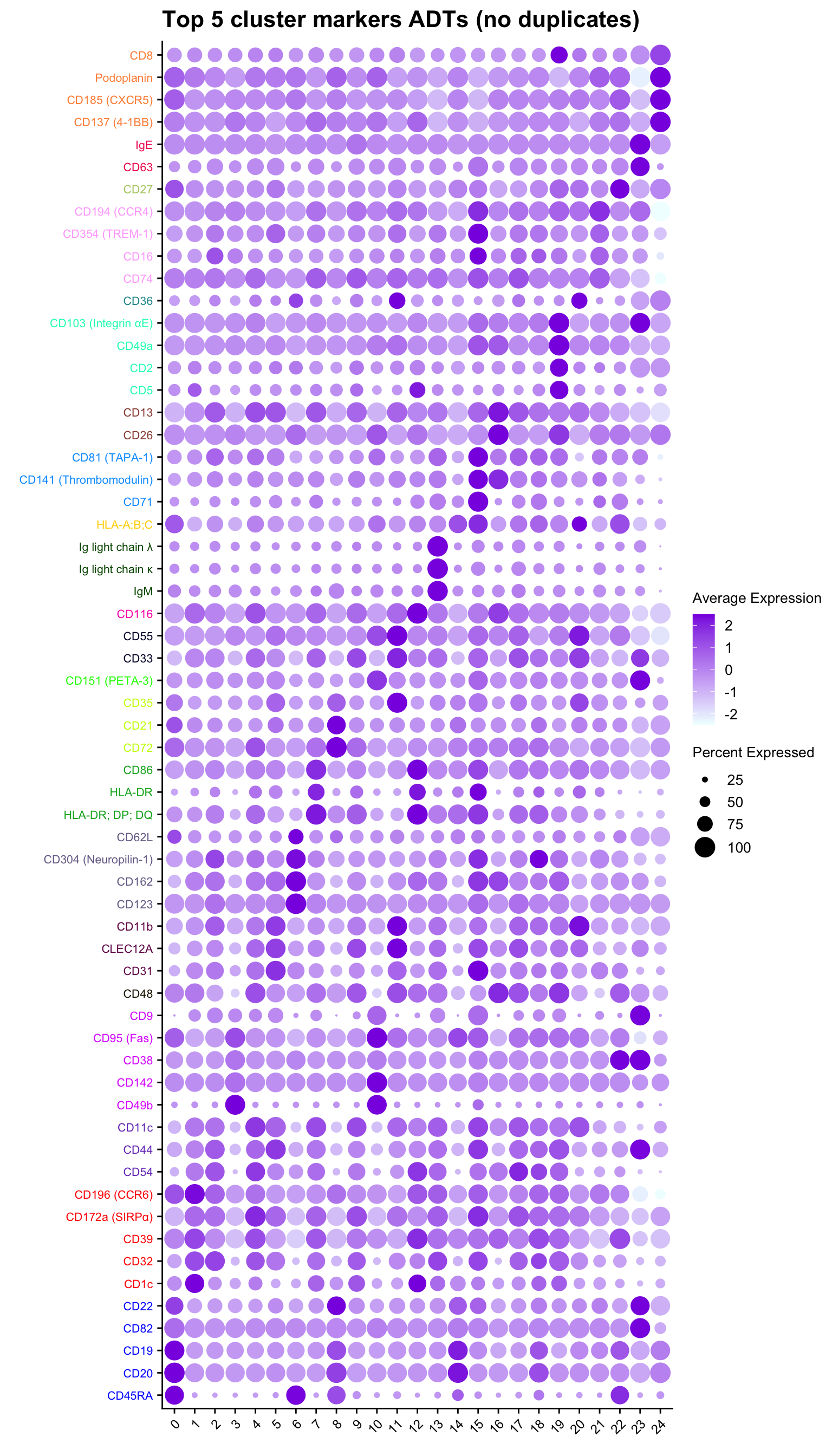
ADT marker heatmap
Make data frame of proteins, clusters, expression levels.
cbind(seuADT@meta.data %>%
        dplyr::select(!!sym(grp)),
      as.data.frame(t(seuADT@assays$ADT.dsb@data))) %>%
  rownames_to_column(var = "cell") %>%
  pivot_longer(c(-!!sym(grp), -cell),
               names_to = "ADT",
               values_to = "expression") %>%
  dplyr::group_by(!!sym(grp), ADT) %>%
  dplyr::summarize(Expression = mean(expression)) %>%
  ungroup() -> dat

# plot expression density to select heatmap colour scale range
plot(density(dat$Expression))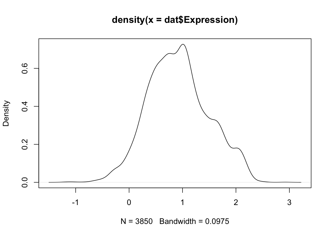
dat %>%
  dplyr::filter(ADT %in% top_markers) |>
  heatmap(
    .column = !!sym(grp),
    .row = ADT,
    .value = Expression,
    row_order = top_markers,
    scale = "none",
    rect_gp = grid::gpar(col = "white", lwd = 1),
    show_row_names = TRUE,
    cluster_columns = FALSE,
    cluster_rows = FALSE,
    column_names_gp = grid::gpar(fontsize = 10),
    column_title_gp = grid::gpar(fontsize = 12),
    row_names_gp = grid::gpar(fontsize = 8, col = cols[order(top_markers)]),
    row_title_gp = grid::gpar(fontsize = 12),
    column_title_side = "top",
    palette_value = circlize::colorRamp2(seq(-0.5, 2.5, length.out = 256),
                                         viridis::magma(256)),
    heatmap_legend_param = list(direction = "vertical"))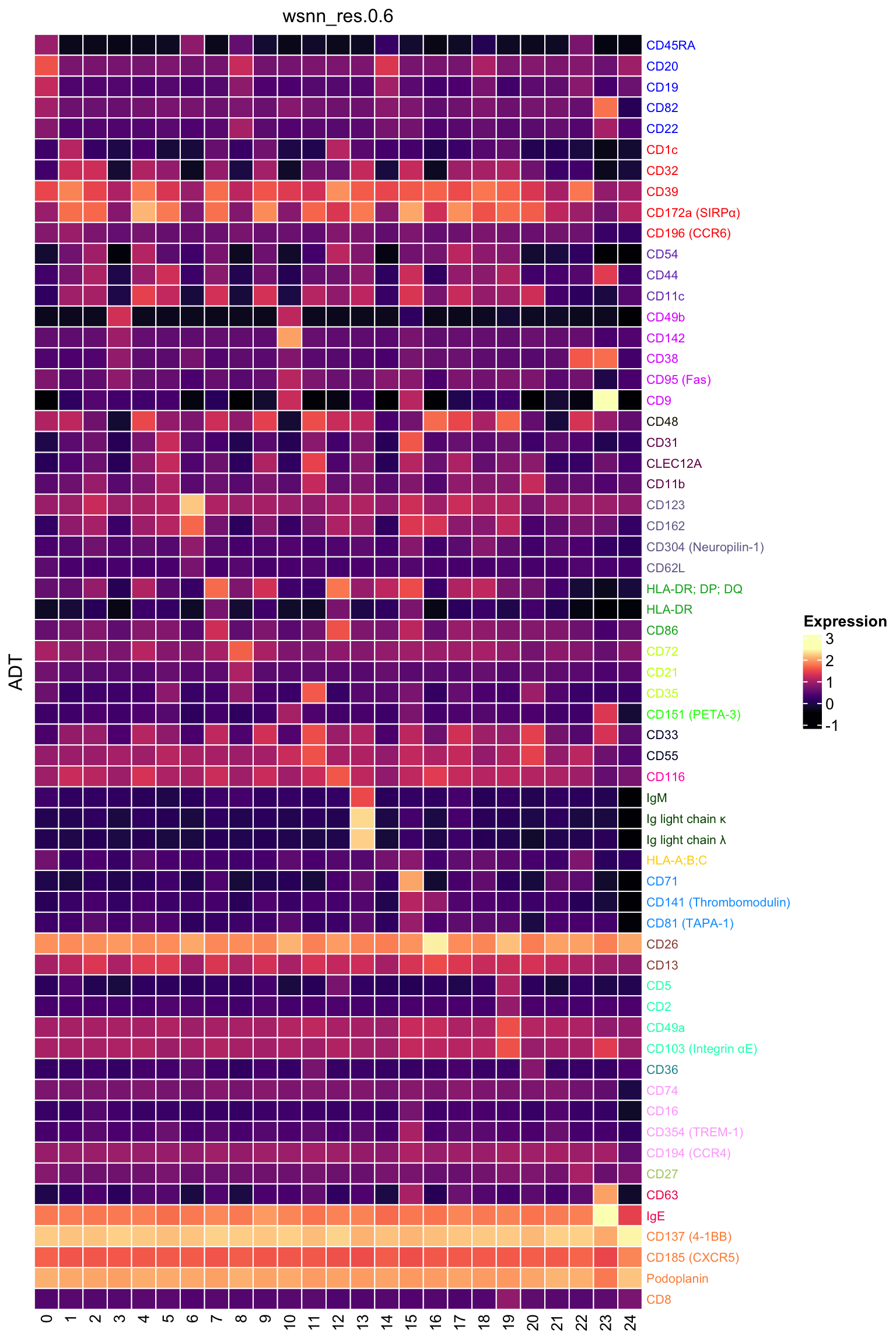
Save ADT markers
options(scipen=-1, digits = 6)
contnames <- colnames(mycont)
dirName <- here("output",
                "cluster_markers",
                glue("ADT{ambient}"),
                "other_cells")
if(!dir.exists(dirName)) dir.create(dirName, recursive = TRUE)

for(c in contnames){
  top <- topTreat(tr, coef = c, n = Inf)
  top <- top[top$logFC > 0, ]
  write.csv(top,
            file = glue("{dirName}/up-cluster-limma-{c}.csv"),
            sep = ",",
            quote = FALSE,
            col.names = NA,
            row.names = TRUE)
}
Session info
sessionInfo()R version 4.3.2 (2023-10-31)
Platform: aarch64-apple-darwin20 (64-bit)
Running under: macOS Sonoma 14.3.1
Matrix products: default
BLAS: /Library/Frameworks/R.framework/Versions/4.3-arm64/Resources/lib/libRblas.0.dylib
LAPACK: /Library/Frameworks/R.framework/Versions/4.3-arm64/Resources/lib/libRlapack.dylib; LAPACK version 3.11.0
locale:
[1] en_US.UTF-8/en_US.UTF-8/en_US.UTF-8/C/en_US.UTF-8/en_US.UTF-8
time zone: Australia/Melbourne
tzcode source: internal
attached base packages:
[1] stats4 stats graphics grDevices datasets utils methods
[8] base
other attached packages:
[1] dsb_1.0.3 tidyHeatmap_1.8.1
[3] speckle_1.2.0 glue_1.7.0
[5] org.Hs.eg.db_3.18.0 AnnotationDbi_1.64.1
[7] patchwork_1.2.0 clustree_0.5.1
[9] ggraph_2.2.0 here_1.0.1
[11] dittoSeq_1.14.2 glmGamPoi_1.14.3
[13] SeuratObject_4.1.4 Seurat_4.4.0
[15] lubridate_1.9.3 forcats_1.0.0
[17] stringr_1.5.1 dplyr_1.1.4
[19] purrr_1.0.2 readr_2.1.5
[21] tidyr_1.3.1 tibble_3.2.1
[23] ggplot2_3.5.0 tidyverse_2.0.0
[25] edgeR_4.0.15 limma_3.58.1
[27] SingleCellExperiment_1.24.0 SummarizedExperiment_1.32.0
[29] Biobase_2.62.0 GenomicRanges_1.54.1
[31] GenomeInfoDb_1.38.6 IRanges_2.36.0
[33] S4Vectors_0.40.2 BiocGenerics_0.48.1
[35] MatrixGenerics_1.14.0 matrixStats_1.2.0
[37] workflowr_1.7.1
loaded via a namespace (and not attached):
[1] fs_1.6.3 spatstat.sparse_3.0-3 bitops_1.0-7
[4] httr_1.4.7 RColorBrewer_1.1-3 doParallel_1.0.17
[7] backports_1.4.1 tools_4.3.2 sctransform_0.4.1
[10] utf8_1.2.4 R6_2.5.1 lazyeval_0.2.2
[13] uwot_0.1.16 GetoptLong_1.0.5 withr_3.0.0
[16] sp_2.1-3 gridExtra_2.3 progressr_0.14.0
[19] cli_3.6.2 Cairo_1.6-2 spatstat.explore_3.2-6
[22] prismatic_1.1.1 labeling_0.4.3 sass_0.4.8
[25] spatstat.data_3.0-4 ggridges_0.5.6 pbapply_1.7-2
[28] parallelly_1.37.0 rstudioapi_0.15.0 RSQLite_2.3.5
[31] generics_0.1.3 shape_1.4.6 vroom_1.6.5
[34] ica_1.0-3 spatstat.random_3.2-2 dendextend_1.17.1
[37] Matrix_1.6-5 ggbeeswarm_0.7.2 fansi_1.0.6
[40] abind_1.4-5 lifecycle_1.0.4 whisker_0.4.1
[43] yaml_2.3.8 SparseArray_1.2.4 Rtsne_0.17
[46] paletteer_1.6.0 grid_4.3.2 blob_1.2.4
[49] promises_1.2.1 crayon_1.5.2 miniUI_0.1.1.1
[52] lattice_0.22-5 cowplot_1.1.3 KEGGREST_1.42.0
[55] pillar_1.9.0 knitr_1.45 ComplexHeatmap_2.18.0
[58] rjson_0.2.21 future.apply_1.11.1 codetools_0.2-19
[61] leiden_0.4.3.1 getPass_0.2-4 data.table_1.15.0
[64] vctrs_0.6.5 png_0.1-8 gtable_0.3.4
[67] rematch2_2.1.2 cachem_1.0.8 xfun_0.42
[70] S4Arrays_1.2.0 mime_0.12 tidygraph_1.3.1
[73] survival_3.5-8 pheatmap_1.0.12 iterators_1.0.14
[76] statmod_1.5.0 ellipsis_0.3.2 fitdistrplus_1.1-11
[79] ROCR_1.0-11 nlme_3.1-164 bit64_4.0.5
[82] RcppAnnoy_0.0.22 rprojroot_2.0.4 bslib_0.6.1
[85] irlba_2.3.5.1 vipor_0.4.7 KernSmooth_2.23-22
[88] colorspace_2.1-0 DBI_1.2.1 ggrastr_1.0.2
[91] tidyselect_1.2.0 processx_3.8.3 bit_4.0.5
[94] compiler_4.3.2 git2r_0.33.0 DelayedArray_0.28.0
[97] plotly_4.10.4 checkmate_2.3.1 scales_1.3.0
[100] lmtest_0.9-40 callr_3.7.3 digest_0.6.34
[103] goftest_1.2-3 spatstat.utils_3.0-4 rmarkdown_2.25
[106] XVector_0.42.0 htmltools_0.5.7 pkgconfig_2.0.3
[109] highr_0.10 fastmap_1.1.1 rlang_1.1.3
[112] GlobalOptions_0.1.2 htmlwidgets_1.6.4 shiny_1.8.0
[115] farver_2.1.1 jquerylib_0.1.4 zoo_1.8-12
[118] jsonlite_1.8.8 mclust_6.1 RCurl_1.98-1.14
[121] magrittr_2.0.3 GenomeInfoDbData_1.2.11 munsell_0.5.0
[124] Rcpp_1.0.12 viridis_0.6.5 reticulate_1.35.0
[127] stringi_1.8.3 zlibbioc_1.48.0 MASS_7.3-60.0.1
[130] plyr_1.8.9 parallel_4.3.2 listenv_0.9.1
[133] ggrepel_0.9.5 deldir_2.0-2 Biostrings_2.70.2
[136] graphlayouts_1.1.0 splines_4.3.2 tensor_1.5
[139] hms_1.1.3 circlize_0.4.15 locfit_1.5-9.8
[142] ps_1.7.6 igraph_2.0.1.1 spatstat.geom_3.2-8
[145] reshape2_1.4.4 evaluate_0.23 renv_1.0.3
[148] tzdb_0.4.0 foreach_1.5.2 tweenr_2.0.3
[151] httpuv_1.6.14 RANN_2.6.1 polyclip_1.10-6
[154] future_1.33.1 clue_0.3-65 scattermore_1.2
[157] ggforce_0.4.2 xtable_1.8-4 later_1.3.2
[160] viridisLite_0.4.2 memoise_2.0.1 beeswarm_0.4.0
[163] cluster_2.1.6 timechange_0.3.0 globals_0.16.2