Last updated: 2024-08-09

Checks: 7 0

Knit directory: paed-inflammation-CITEseq/

This reproducible R Markdown analysis was created with workflowr (version 1.7.1). The Checks tab describes the reproducibility checks that were applied when the results were created. The Past versions tab lists the development history.

R Markdown file: up-to-date

Great! Since the R Markdown file has been committed to the Git repository, you know the exact version of the code that produced these results.

Environment: empty

Great job! The global environment was empty. Objects defined in the global environment can affect the analysis in your R Markdown file in unknown ways. For reproduciblity it’s best to always run the code in an empty environment.

Seed: set.seed(20240216)

The command set.seed(20240216) was run prior to running the code in the R Markdown file. Setting a seed ensures that any results that rely on randomness, e.g. subsampling or permutations, are reproducible.

Session information: recorded

Great job! Recording the operating system, R version, and package versions is critical for reproducibility.

Cache: none

Nice! There were no cached chunks for this analysis, so you can be confident that you successfully produced the results during this run.

File paths: relative

Great job! Using relative paths to the files within your workflowr project makes it easier to run your code on other machines.

Repository version: 01f0f43

Great! You are using Git for version control. Tracking code development and connecting the code version to the results is critical for reproducibility.

The results in this page were generated with repository version 01f0f43. See the Past versions tab to see a history of the changes made to the R Markdown and HTML files.

Note that you need to be careful to ensure that all relevant files for the analysis have been committed to Git prior to generating the results (you can use wflow_publish or wflow_git_commit). workflowr only checks the R Markdown file, but you know if there are other scripts or data files that it depends on. Below is the status of the Git repository when the results were generated:


Ignored files:
    Ignored:    .Rhistory
    Ignored:    .Rproj.user/
    Ignored:    code/voomByGroup/
    Ignored:    data/.DS_Store
    Ignored:    data/C133_Neeland/
    Ignored:    data/C133_Neeland_batch0/
    Ignored:    data/C133_Neeland_batch1/
    Ignored:    data/C133_Neeland_batch2/
    Ignored:    data/C133_Neeland_batch3/
    Ignored:    data/C133_Neeland_batch4/
    Ignored:    data/C133_Neeland_batch5/
    Ignored:    data/C133_Neeland_batch6/
    Ignored:    data/C133_Neeland_merged/
    Ignored:    renv/library/
    Ignored:    renv/staging/

Untracked files:
    Untracked:  analysis/13.1_DGE_analysis_macro-alveolar_cells_decontx.Rmd
    Untracked:  code/cellbender.sh
    Untracked:  code/move_files.R
    Untracked:  data/heart10k_raw_feature_bc_matrix.h5
    Untracked:  data/oshlack_lab/
    Untracked:  data/output.log
    Untracked:  data/tiny_output.log
    Untracked:  data/tiny_raw_feature_bc_matrix.h5ad

Unstaged changes:
    Modified:   .DS_Store
    Modified:   analysis/06.1_azimuth_annotation_decontx.Rmd
    Modified:   code/run_cellbender.R

Note that any generated files, e.g. HTML, png, CSS, etc., are not included in this status report because it is ok for generated content to have uncommitted changes.

These are the previous versions of the repository in which changes were made to the R Markdown (analysis/14.0_proportions_analysis_broad.Rmd) and HTML (docs/14.0_proportions_analysis_broad.html) files. If you’ve configured a remote Git repository (see ?wflow_git_remote), click on the hyperlinks in the table below to view the files as they were in that past version.

File	Version	Author	Date	Message
Rmd	01f0f43	Jovana Maksimovic	2024-08-09	wflow_publish("analysis/14.*")

Load libraries

suppressPackageStartupMessages({
  library(SingleCellExperiment)
  library(edgeR)
  library(tidyverse)
  library(ggplot2)
  library(Seurat)
  library(glmGamPoi)
  library(dittoSeq)
  library(clustree)
  library(AnnotationDbi)
  library(org.Hs.eg.db)
  library(glue)
  library(speckle)
  library(patchwork)
  library(paletteer)
  library(tidyHeatmap)
  library(here)
})

set.seed(42)
options(scipen=999)
options(future.globals.maxSize = 6500 * 1024^2)

Load Data

files <- list.files(here("data/C133_Neeland_merged"),
                    pattern = "C133_Neeland_full_clean.*(macrophages|t_cells|other_cells)_annotated_diet.SEU.rds",
                    full.names = TRUE)

seuLst <- lapply(files[2:4], function(f) readRDS(f))

seu <- merge(seuLst[[1]], 
             y = c(seuLst[[2]], 
                   seuLst[[3]]))
seu

An object of class Seurat 
21568 features across 191521 samples within 1 assay 
Active assay: RNA (21568 features, 0 variable features)

             used    (Mb) gc trigger    (Mb) limit (Mb)   max used    (Mb)
Ncells   10360801   553.4   18225151   973.4         NA   13595624   726.1
Vcells 1328307424 10134.2 3629547812 27691.3      65536 3489906798 26625.9

Analyse Cell type proportions

# Differences in cell type proportions
props <- getTransformedProps(clusters = seu$Broad,
                             sample = seu$sample.id, transform="asin")
props$Proportions %>% knitr::kable()

	sample_1.1	sample_15.1	sample_16.1	sample_17.1	sample_18.1	sample_19.1	sample_2.1	sample_20.1	sample_21.1	sample_22.1	sample_23.1	sample_24.1	sample_25.1	sample_26.1	sample_27.1	sample_28.1	sample_29.1	sample_3.1	sample_30.1	sample_31.1	sample_32.1	sample_33.1	sample_34.1	sample_34.2	sample_34.3	sample_35.1	sample_35.2	sample_36.1	sample_36.2	sample_37.1	sample_37.2	sample_37.3	sample_38.1	sample_38.2	sample_38.3	sample_39.1	sample_39.2	sample_4.1	sample_40.1	sample_41.1	sample_42.1	sample_43.1	sample_5.1	sample_6.1	sample_7.1
B cells	0.0223723	0.0071704	0.0018883	0.0428725	0.0015235	0.0023866	0.0950689	0.0017933	0.0095134	0.0023447	0.2436149	0.0057254	0.0027506	0.0122549	0.0020268	0.0006984	0.0918367	0.0119505	0.0064935	0.0041667	0.0027000	0.0607761	0.0026738	0.0000000	0.0016584	0.0181452	0.0081239	0.0304653	0.0502624	0.0069589	0.0124824	0.0105605	0.0048374	0.0058787	0.0356175	0.0434431	0.0275087	0.0096690	0.0000000	0.0000000	0.0000000	0.0000000	0.0181922	0.0046205	0.0282528
CD4 T cells	0.0092866	0.0275786	0.0129485	0.0176849	0.0082267	0.0023866	0.0364283	0.0087101	0.0192097	0.0082063	0.1650295	0.0262504	0.0174205	0.0323529	0.0133766	0.0060064	0.0299745	0.0061886	0.1911977	0.0722222	0.0155248	0.1547452	0.0113636	0.0051207	0.0035537	0.0173387	0.0164368	0.0113827	0.0425297	0.0153097	0.0163076	0.0268075	0.0056436	0.0102104	0.0274874	0.0250944	0.0585045	0.0106607	0.1434307	0.0584656	0.0374161	0.0462648	0.0801592	0.0137671	0.0381306
CD8 T cells	0.0063318	0.0295091	0.0283248	0.0353698	0.0164534	0.0011933	0.0510884	0.0098629	0.0179290	0.0095252	0.1277014	0.0310036	0.0134474	0.0308824	0.0267531	0.0153653	0.0586735	0.0091763	0.0977633	0.0949074	0.0175498	0.1280972	0.0100267	0.0029261	0.0052120	0.0203629	0.0102022	0.0033478	0.0248550	0.0146138	0.0074492	0.0199025	0.0037624	0.0049505	0.0251645	0.0070157	0.0730337	0.0254122	0.1000000	0.0743386	0.0896167	0.2072391	0.0949403	0.0271570	0.0380244
DC cells	0.0097087	0.0184777	0.0037766	0.0391211	0.0173675	0.0055688	0.0017770	0.0067888	0.0080498	0.0016120	0.0628684	0.0398617	0.0201711	0.0230392	0.0162140	0.0065652	0.0440051	0.0147247	0.0497835	0.0157407	0.0121498	0.0719963	0.0788770	0.0643745	0.0322199	0.0219758	0.0251275	0.0348175	0.0544049	0.0073069	0.0062412	0.0048741	0.0010750	0.0024752	0.0081301	0.0232056	0.0350639	0.0126441	0.0000000	0.0000000	0.0000000	0.0000000	0.0204662	0.0045262	0.0059480
dividing innate cells	0.0000000	0.0002758	0.0002698	0.0024116	0.0006094	0.0003978	0.0093292	0.0002562	0.0000000	0.0000000	0.0108055	0.0012963	0.0006112	0.0000000	0.0000000	0.0001397	0.0031888	0.0006402	0.0003608	0.0000000	0.0003375	0.0032726	0.0013369	0.0000000	0.0002369	0.0002016	0.0001889	0.0016739	0.0008285	0.0000000	0.0000000	0.0004062	0.0000000	0.0003094	0.0011614	0.0035078	0.0017435	0.0006198	0.0000000	0.0000000	0.0000000	0.0000000	0.0000000	0.0000000	0.0001062
epithelial cells	0.0426340	0.0132377	0.0005395	0.0032154	0.0053321	0.0019889	0.1537095	0.0043551	0.0104281	0.0038101	0.2092338	0.0034568	0.0006112	0.0034314	0.0275638	0.0006984	0.0446429	0.0017072	0.0010823	0.0018519	0.0000000	0.0219729	0.0093583	0.0087783	0.0037906	0.0094758	0.0094464	0.0077000	0.0038663	0.0076548	0.0020133	0.0052803	0.0016125	0.0018564	0.0154859	0.0029682	0.0069740	0.0032230	0.0000000	0.0000000	0.0000000	0.0000000	0.0062536	0.0012258	0.0011683
gamma delta T cells	0.0000000	0.0005516	0.0008093	0.0008039	0.0003047	0.0000000	0.0000000	0.0003843	0.0007318	0.0000000	0.0000000	0.0003241	0.0006112	0.0004902	0.0012161	0.0001397	0.0000000	0.0000000	0.0223665	0.0064815	0.0003375	0.0014025	0.0000000	0.0000000	0.0000000	0.0002016	0.0000000	0.0003348	0.0000000	0.0010438	0.0000000	0.0000000	0.0000000	0.0003094	0.0038715	0.0002698	0.0027121	0.0000000	0.0171533	0.0029101	0.0028432	0.0017689	0.0005685	0.0000000	0.0009559
innate lymphocyte	0.0029548	0.0353006	0.0045859	0.0077706	0.0039610	0.0023866	0.0075522	0.0019214	0.0012806	0.0038101	0.0245580	0.0046451	0.0058068	0.0083333	0.0044589	0.0006984	0.0082908	0.0014938	0.0339105	0.0129630	0.0006750	0.0144928	0.0006684	0.0007315	0.0016584	0.0036290	0.0039675	0.0006696	0.0138083	0.0013918	0.0018120	0.0020309	0.0002687	0.0003094	0.0046458	0.0010793	0.0048431	0.0047105	0.0229927	0.0177249	0.0378710	0.0168730	0.0136441	0.0071664	0.0023367
Macrophages	0.8518362	0.8019857	0.9072026	0.7607181	0.8740098	0.9240255	0.6010662	0.9126425	0.8940724	0.9422626	0.1070727	0.7980987	0.8719438	0.8401961	0.8479935	0.9353262	0.6696429	0.9026889	0.5313853	0.7277778	0.8876139	0.4684432	0.8288770	0.8580834	0.8995499	0.8252016	0.8730399	0.7937730	0.7321182	0.9060543	0.8969197	0.9102356	0.9180328	0.9260520	0.8180410	0.8345926	0.7268501	0.8098426	0.6857664	0.7878307	0.7939270	0.6871683	0.7072200	0.8938237	0.8326075
mast cells	0.0000000	0.0000000	0.0000000	0.0005359	0.0001523	0.0000000	0.0008885	0.0000000	0.0000000	0.0000000	0.0098232	0.0001080	0.0012225	0.0014706	0.0008107	0.0000000	0.0063776	0.0000000	0.0007215	0.0023148	0.0000000	0.0112202	0.0000000	0.0000000	0.0004738	0.0004032	0.0003779	0.0010044	0.0000000	0.0000000	0.0000000	0.0004062	0.0002687	0.0000000	0.0007743	0.0002698	0.0001937	0.0021074	0.0000000	0.0000000	0.0000000	0.0000000	0.0005685	0.0000000	0.0000000
monocytes	0.0113972	0.0013789	0.0013488	0.0200965	0.0195003	0.0023866	0.0035540	0.0044832	0.0012806	0.0013189	0.0098232	0.0468834	0.0097800	0.0127451	0.0097284	0.0108954	0.0114796	0.0134443	0.0119048	0.0087963	0.0155248	0.0107527	0.0106952	0.0065838	0.0073442	0.0217742	0.0171925	0.0133914	0.0265120	0.0059151	0.0094625	0.0064988	0.0037624	0.0046411	0.0061943	0.0218564	0.0240217	0.1063592	0.0000000	0.0000000	0.0000000	0.0000000	0.0187607	0.0086752	0.0065852
neutrophils	0.0000000	0.0000000	0.0000000	0.0056270	0.0012188	0.0000000	0.0000000	0.0001281	0.0000000	0.0000000	0.0108055	0.0006482	0.0003056	0.0014706	0.0000000	0.0004191	0.0063776	0.0004268	0.0010823	0.0013889	0.0006750	0.0229079	0.0033422	0.0051207	0.0021322	0.0022177	0.0005668	0.0549046	0.0035902	0.0003479	0.0004027	0.0012185	0.0000000	0.0003094	0.0000000	0.0089045	0.0092987	0.0004958	0.0000000	0.0000000	0.0000000	0.0000000	0.0000000	0.0000000	0.0000000
NK cells	0.0046433	0.0085494	0.0051254	0.0058950	0.0036563	0.0000000	0.0026655	0.0014090	0.0020124	0.0011723	0.0157171	0.0016204	0.0015281	0.0014706	0.0008107	0.0000000	0.0044643	0.0014938	0.0266955	0.0060185	0.0016875	0.0079476	0.0020053	0.0000000	0.0002369	0.0020161	0.0011336	0.0010044	0.0033140	0.0003479	0.0004027	0.0012185	0.0013437	0.0006188	0.0011614	0.0000000	0.0019372	0.0019834	0.0175182	0.0100529	0.0068236	0.0073479	0.0068221	0.0005658	0.0098779
NK-T cells	0.0000000	0.0041368	0.0002698	0.0005359	0.0001523	0.0000000	0.0013327	0.0002562	0.0005488	0.0001465	0.0019646	0.0000000	0.0003056	0.0014706	0.0000000	0.0001397	0.0012755	0.0002134	0.0014430	0.0000000	0.0000000	0.0014025	0.0000000	0.0000000	0.0000000	0.0004032	0.0011336	0.0000000	0.0005523	0.0003479	0.0000000	0.0000000	0.0000000	0.0000000	0.0000000	0.0000000	0.0007749	0.0000000	0.0025547	0.0002646	0.0004549	0.0010886	0.0005685	0.0000943	0.0009559
Proliferating macrophages	0.0367244	0.0493657	0.0321014	0.0560021	0.0467703	0.0572792	0.0310973	0.0462406	0.0332967	0.0247655	0.0000000	0.0392136	0.0531785	0.0303922	0.0490474	0.0222098	0.0197704	0.0354247	0.0151515	0.0444444	0.0445494	0.0187003	0.0407754	0.0475494	0.0414594	0.0556452	0.0317400	0.0451958	0.0425297	0.0320111	0.0457016	0.0097482	0.0588551	0.0411510	0.0514905	0.0275229	0.0236343	0.0115284	0.0083942	0.0473545	0.0268395	0.0312968	0.0278567	0.0375295	0.0333510
proliferating T/NK	0.0021106	0.0024821	0.0008093	0.0013398	0.0007617	0.0000000	0.0044425	0.0007685	0.0016465	0.0010258	0.0009823	0.0008642	0.0003056	0.0000000	0.0000000	0.0006984	0.0000000	0.0004268	0.0086580	0.0009259	0.0006750	0.0018700	0.0000000	0.0007315	0.0004738	0.0010081	0.0013225	0.0003348	0.0008285	0.0006959	0.0008053	0.0008123	0.0005375	0.0009282	0.0007743	0.0002698	0.0029059	0.0007438	0.0021898	0.0010582	0.0042079	0.0009525	0.0039795	0.0008487	0.0016994

Cell type proportions by sample

props$Proportions %>%
  data.frame %>%
  inner_join(seu@meta.data %>%
               dplyr::select(sample.id, 
                             Disease,
                             Treatment,
                             Status, 
                             Severity,
                             Group,
                             Batch, 
                             Age, 
                             Sex), 
             by = c("sample" = "sample.id")) %>%
  distinct()-> dat

ggplot(dat, aes(x = sample, y = Freq, fill = clusters)) +
  geom_bar(stat = "identity", color = "black", size = 0.1) +
  theme(axis.text.x = element_text(angle = 90,
                                   vjust = 0.5,
                                   hjust = 1),
        legend.text = element_text(size = 8),
        legend.position = "bottom") +
  labs(y = "Proportion", fill = "Cell Label") +
  scale_fill_paletteer_d("miscpalettes::pastel", direction = 1) +
  facet_grid(~Group, scales = "free_x", space = "free_x")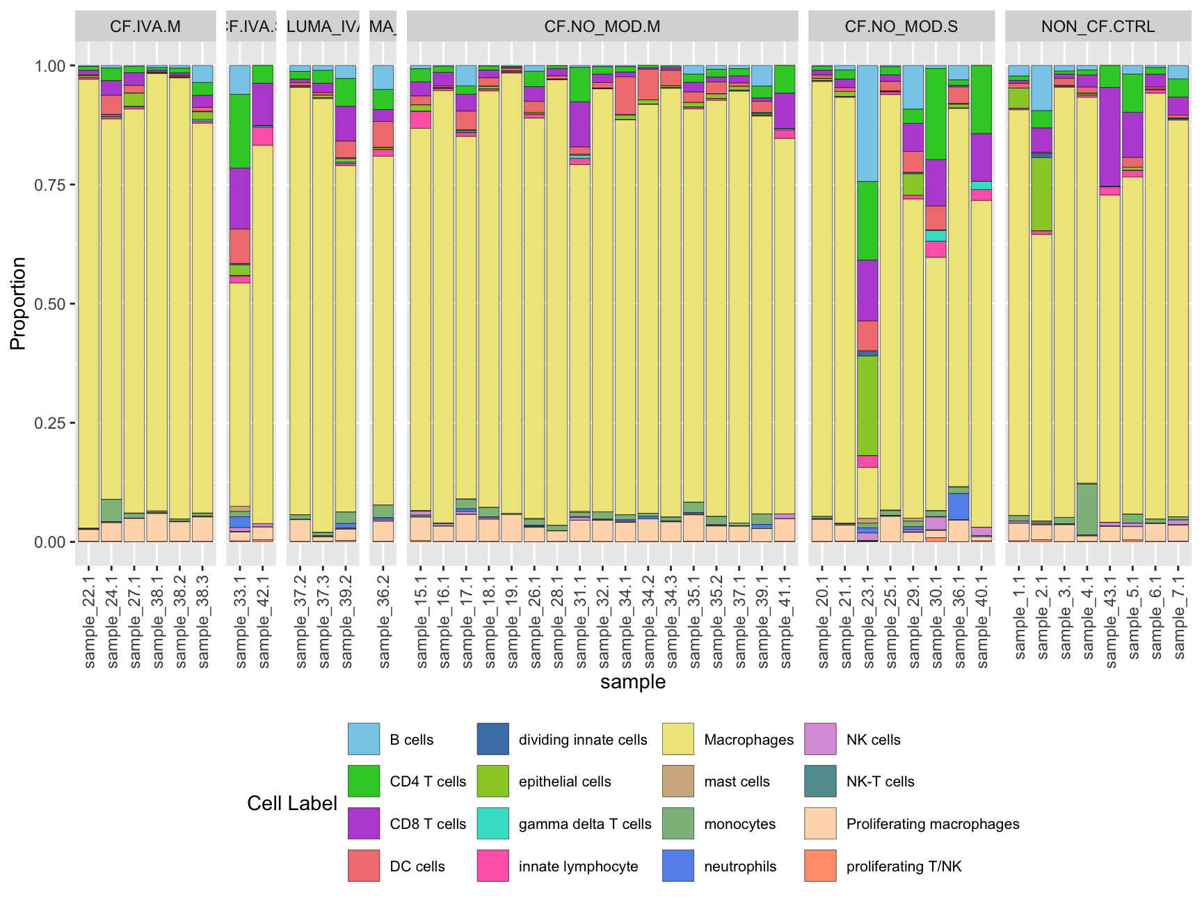

No. cells per sample

props$Counts %>%
  data.frame %>%
  inner_join(seu@meta.data %>%
               dplyr::select(sample.id, 
                             Disease,
                             Treatment,
                             Status, 
                             Severity, 
                             Group,
                             Batch, 
                             Age, 
                             Sex), 
             by = c("sample" = "sample.id")) %>%
  distinct() -> dat

ggplot(dat, aes(x = sample, y = Freq, fill = Disease)) +
  geom_bar(stat = "identity") +
  theme(axis.text.x = element_text(angle = 90,
                                   vjust = 0.5,
                                   hjust = 1),
        legend.text = element_text(size = 8),
        legend.position = "bottom") +
  labs(y = "No. cells", fill = "Disease") +
  facet_grid(~Group, scales = "free_x", space = "free_x") +
  geom_hline(yintercept = 1000, linetype = "dashed")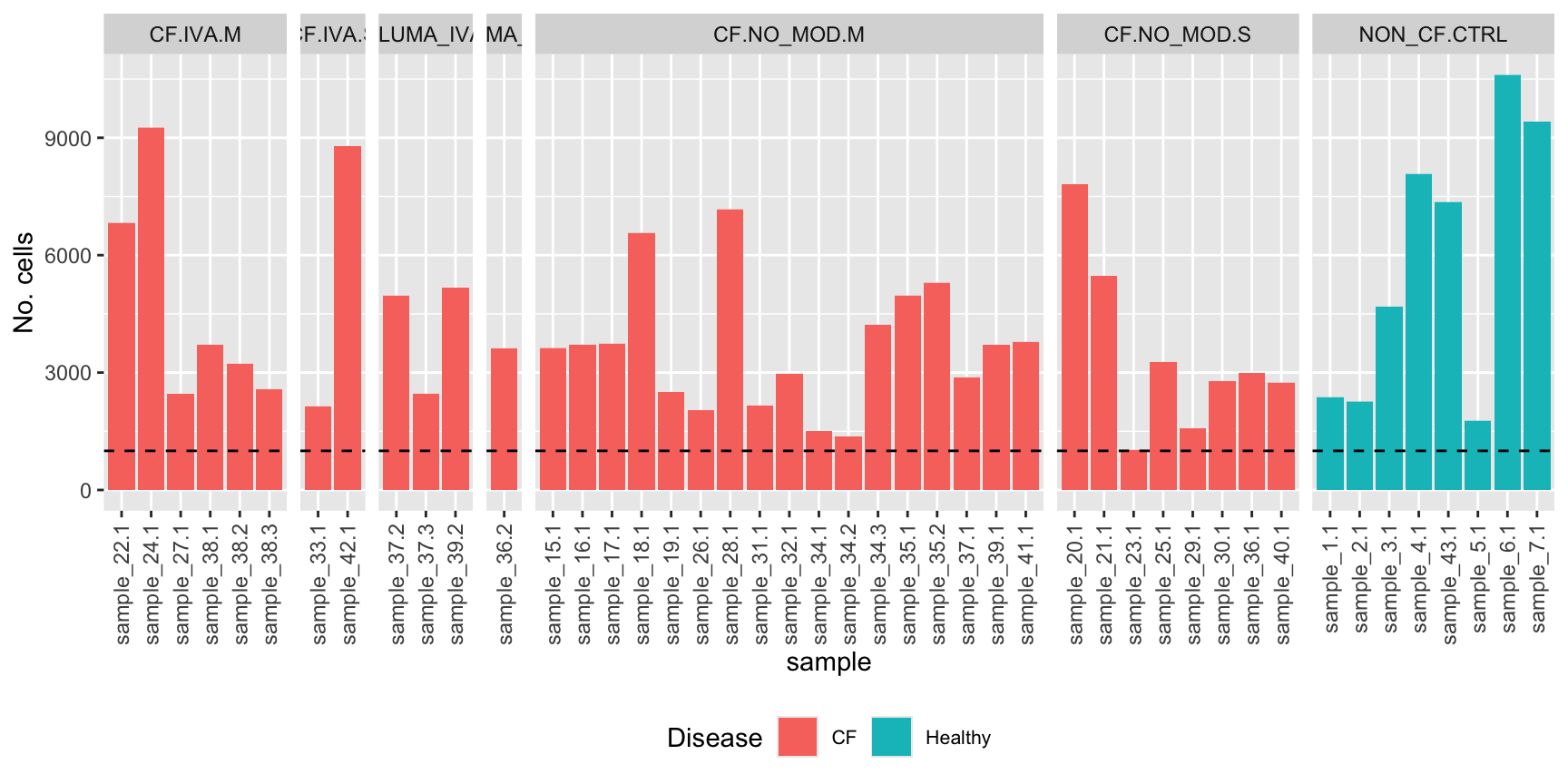

Remove sample with too few cells.

seu <- subset(seu, cells = which(!seu$sample.id %in% c("sample_23.1")))

# Differences in cell type proportions
props <- getTransformedProps(clusters = seu$Broad,
                             sample = seu$sample.id, transform="asin")
props$Proportions %>% knitr::kable()

	sample_1.1	sample_15.1	sample_16.1	sample_17.1	sample_18.1	sample_19.1	sample_2.1	sample_20.1	sample_21.1	sample_22.1	sample_24.1	sample_25.1	sample_26.1	sample_27.1	sample_28.1	sample_29.1	sample_3.1	sample_30.1	sample_31.1	sample_32.1	sample_33.1	sample_34.1	sample_34.2	sample_34.3	sample_35.1	sample_35.2	sample_36.1	sample_36.2	sample_37.1	sample_37.2	sample_37.3	sample_38.1	sample_38.2	sample_38.3	sample_39.1	sample_39.2	sample_4.1	sample_40.1	sample_41.1	sample_42.1	sample_43.1	sample_5.1	sample_6.1	sample_7.1
B cells	0.0223723	0.0071704	0.0018883	0.0428725	0.0015235	0.0023866	0.0950689	0.0017933	0.0095134	0.0023447	0.0057254	0.0027506	0.0122549	0.0020268	0.0006984	0.0918367	0.0119505	0.0064935	0.0041667	0.0027000	0.0607761	0.0026738	0.0000000	0.0016584	0.0181452	0.0081239	0.0304653	0.0502624	0.0069589	0.0124824	0.0105605	0.0048374	0.0058787	0.0356175	0.0434431	0.0275087	0.0096690	0.0000000	0.0000000	0.0000000	0.0000000	0.0181922	0.0046205	0.0282528
CD4 T cells	0.0092866	0.0275786	0.0129485	0.0176849	0.0082267	0.0023866	0.0364283	0.0087101	0.0192097	0.0082063	0.0262504	0.0174205	0.0323529	0.0133766	0.0060064	0.0299745	0.0061886	0.1911977	0.0722222	0.0155248	0.1547452	0.0113636	0.0051207	0.0035537	0.0173387	0.0164368	0.0113827	0.0425297	0.0153097	0.0163076	0.0268075	0.0056436	0.0102104	0.0274874	0.0250944	0.0585045	0.0106607	0.1434307	0.0584656	0.0374161	0.0462648	0.0801592	0.0137671	0.0381306
CD8 T cells	0.0063318	0.0295091	0.0283248	0.0353698	0.0164534	0.0011933	0.0510884	0.0098629	0.0179290	0.0095252	0.0310036	0.0134474	0.0308824	0.0267531	0.0153653	0.0586735	0.0091763	0.0977633	0.0949074	0.0175498	0.1280972	0.0100267	0.0029261	0.0052120	0.0203629	0.0102022	0.0033478	0.0248550	0.0146138	0.0074492	0.0199025	0.0037624	0.0049505	0.0251645	0.0070157	0.0730337	0.0254122	0.1000000	0.0743386	0.0896167	0.2072391	0.0949403	0.0271570	0.0380244
DC cells	0.0097087	0.0184777	0.0037766	0.0391211	0.0173675	0.0055688	0.0017770	0.0067888	0.0080498	0.0016120	0.0398617	0.0201711	0.0230392	0.0162140	0.0065652	0.0440051	0.0147247	0.0497835	0.0157407	0.0121498	0.0719963	0.0788770	0.0643745	0.0322199	0.0219758	0.0251275	0.0348175	0.0544049	0.0073069	0.0062412	0.0048741	0.0010750	0.0024752	0.0081301	0.0232056	0.0350639	0.0126441	0.0000000	0.0000000	0.0000000	0.0000000	0.0204662	0.0045262	0.0059480
dividing innate cells	0.0000000	0.0002758	0.0002698	0.0024116	0.0006094	0.0003978	0.0093292	0.0002562	0.0000000	0.0000000	0.0012963	0.0006112	0.0000000	0.0000000	0.0001397	0.0031888	0.0006402	0.0003608	0.0000000	0.0003375	0.0032726	0.0013369	0.0000000	0.0002369	0.0002016	0.0001889	0.0016739	0.0008285	0.0000000	0.0000000	0.0004062	0.0000000	0.0003094	0.0011614	0.0035078	0.0017435	0.0006198	0.0000000	0.0000000	0.0000000	0.0000000	0.0000000	0.0000000	0.0001062
epithelial cells	0.0426340	0.0132377	0.0005395	0.0032154	0.0053321	0.0019889	0.1537095	0.0043551	0.0104281	0.0038101	0.0034568	0.0006112	0.0034314	0.0275638	0.0006984	0.0446429	0.0017072	0.0010823	0.0018519	0.0000000	0.0219729	0.0093583	0.0087783	0.0037906	0.0094758	0.0094464	0.0077000	0.0038663	0.0076548	0.0020133	0.0052803	0.0016125	0.0018564	0.0154859	0.0029682	0.0069740	0.0032230	0.0000000	0.0000000	0.0000000	0.0000000	0.0062536	0.0012258	0.0011683
gamma delta T cells	0.0000000	0.0005516	0.0008093	0.0008039	0.0003047	0.0000000	0.0000000	0.0003843	0.0007318	0.0000000	0.0003241	0.0006112	0.0004902	0.0012161	0.0001397	0.0000000	0.0000000	0.0223665	0.0064815	0.0003375	0.0014025	0.0000000	0.0000000	0.0000000	0.0002016	0.0000000	0.0003348	0.0000000	0.0010438	0.0000000	0.0000000	0.0000000	0.0003094	0.0038715	0.0002698	0.0027121	0.0000000	0.0171533	0.0029101	0.0028432	0.0017689	0.0005685	0.0000000	0.0009559
innate lymphocyte	0.0029548	0.0353006	0.0045859	0.0077706	0.0039610	0.0023866	0.0075522	0.0019214	0.0012806	0.0038101	0.0046451	0.0058068	0.0083333	0.0044589	0.0006984	0.0082908	0.0014938	0.0339105	0.0129630	0.0006750	0.0144928	0.0006684	0.0007315	0.0016584	0.0036290	0.0039675	0.0006696	0.0138083	0.0013918	0.0018120	0.0020309	0.0002687	0.0003094	0.0046458	0.0010793	0.0048431	0.0047105	0.0229927	0.0177249	0.0378710	0.0168730	0.0136441	0.0071664	0.0023367
Macrophages	0.8518362	0.8019857	0.9072026	0.7607181	0.8740098	0.9240255	0.6010662	0.9126425	0.8940724	0.9422626	0.7980987	0.8719438	0.8401961	0.8479935	0.9353262	0.6696429	0.9026889	0.5313853	0.7277778	0.8876139	0.4684432	0.8288770	0.8580834	0.8995499	0.8252016	0.8730399	0.7937730	0.7321182	0.9060543	0.8969197	0.9102356	0.9180328	0.9260520	0.8180410	0.8345926	0.7268501	0.8098426	0.6857664	0.7878307	0.7939270	0.6871683	0.7072200	0.8938237	0.8326075
mast cells	0.0000000	0.0000000	0.0000000	0.0005359	0.0001523	0.0000000	0.0008885	0.0000000	0.0000000	0.0000000	0.0001080	0.0012225	0.0014706	0.0008107	0.0000000	0.0063776	0.0000000	0.0007215	0.0023148	0.0000000	0.0112202	0.0000000	0.0000000	0.0004738	0.0004032	0.0003779	0.0010044	0.0000000	0.0000000	0.0000000	0.0004062	0.0002687	0.0000000	0.0007743	0.0002698	0.0001937	0.0021074	0.0000000	0.0000000	0.0000000	0.0000000	0.0005685	0.0000000	0.0000000
monocytes	0.0113972	0.0013789	0.0013488	0.0200965	0.0195003	0.0023866	0.0035540	0.0044832	0.0012806	0.0013189	0.0468834	0.0097800	0.0127451	0.0097284	0.0108954	0.0114796	0.0134443	0.0119048	0.0087963	0.0155248	0.0107527	0.0106952	0.0065838	0.0073442	0.0217742	0.0171925	0.0133914	0.0265120	0.0059151	0.0094625	0.0064988	0.0037624	0.0046411	0.0061943	0.0218564	0.0240217	0.1063592	0.0000000	0.0000000	0.0000000	0.0000000	0.0187607	0.0086752	0.0065852
neutrophils	0.0000000	0.0000000	0.0000000	0.0056270	0.0012188	0.0000000	0.0000000	0.0001281	0.0000000	0.0000000	0.0006482	0.0003056	0.0014706	0.0000000	0.0004191	0.0063776	0.0004268	0.0010823	0.0013889	0.0006750	0.0229079	0.0033422	0.0051207	0.0021322	0.0022177	0.0005668	0.0549046	0.0035902	0.0003479	0.0004027	0.0012185	0.0000000	0.0003094	0.0000000	0.0089045	0.0092987	0.0004958	0.0000000	0.0000000	0.0000000	0.0000000	0.0000000	0.0000000	0.0000000
NK cells	0.0046433	0.0085494	0.0051254	0.0058950	0.0036563	0.0000000	0.0026655	0.0014090	0.0020124	0.0011723	0.0016204	0.0015281	0.0014706	0.0008107	0.0000000	0.0044643	0.0014938	0.0266955	0.0060185	0.0016875	0.0079476	0.0020053	0.0000000	0.0002369	0.0020161	0.0011336	0.0010044	0.0033140	0.0003479	0.0004027	0.0012185	0.0013437	0.0006188	0.0011614	0.0000000	0.0019372	0.0019834	0.0175182	0.0100529	0.0068236	0.0073479	0.0068221	0.0005658	0.0098779
NK-T cells	0.0000000	0.0041368	0.0002698	0.0005359	0.0001523	0.0000000	0.0013327	0.0002562	0.0005488	0.0001465	0.0000000	0.0003056	0.0014706	0.0000000	0.0001397	0.0012755	0.0002134	0.0014430	0.0000000	0.0000000	0.0014025	0.0000000	0.0000000	0.0000000	0.0004032	0.0011336	0.0000000	0.0005523	0.0003479	0.0000000	0.0000000	0.0000000	0.0000000	0.0000000	0.0000000	0.0007749	0.0000000	0.0025547	0.0002646	0.0004549	0.0010886	0.0005685	0.0000943	0.0009559
Proliferating macrophages	0.0367244	0.0493657	0.0321014	0.0560021	0.0467703	0.0572792	0.0310973	0.0462406	0.0332967	0.0247655	0.0392136	0.0531785	0.0303922	0.0490474	0.0222098	0.0197704	0.0354247	0.0151515	0.0444444	0.0445494	0.0187003	0.0407754	0.0475494	0.0414594	0.0556452	0.0317400	0.0451958	0.0425297	0.0320111	0.0457016	0.0097482	0.0588551	0.0411510	0.0514905	0.0275229	0.0236343	0.0115284	0.0083942	0.0473545	0.0268395	0.0312968	0.0278567	0.0375295	0.0333510
proliferating T/NK	0.0021106	0.0024821	0.0008093	0.0013398	0.0007617	0.0000000	0.0044425	0.0007685	0.0016465	0.0010258	0.0008642	0.0003056	0.0000000	0.0000000	0.0006984	0.0000000	0.0004268	0.0086580	0.0009259	0.0006750	0.0018700	0.0000000	0.0007315	0.0004738	0.0010081	0.0013225	0.0003348	0.0008285	0.0006959	0.0008053	0.0008123	0.0005375	0.0009282	0.0007743	0.0002698	0.0029059	0.0007438	0.0021898	0.0010582	0.0042079	0.0009525	0.0039795	0.0008487	0.0016994

Cell proportions by sample

props$Proportions %>%
  data.frame %>%
  inner_join(seu@meta.data %>%
               dplyr::select(sample.id, 
                             Disease,
                             Treatment,
                             Status, 
                             Severity, 
                             Group,
                             Batch, 
                             Age, 
                             Sex), 
             by = c("sample" = "sample.id")) %>%
  distinct()-> dat

ggplot(dat, aes(x = sample, y = Freq, fill = clusters)) +
  geom_bar(stat = "identity", color = "black", size = 0.1) +
  theme(axis.text.x = element_text(angle = 90,
                                   vjust = 0.5,
                                   hjust = 1),
        legend.text = element_text(size = 8),
        legend.position = "bottom") +
  labs(y = "Proportion", fill = "Cell Label") +
  scale_fill_paletteer_d("miscpalettes::pastel", direction = 1) +
  facet_grid(~Group, scales = "free_x", space = "free_x")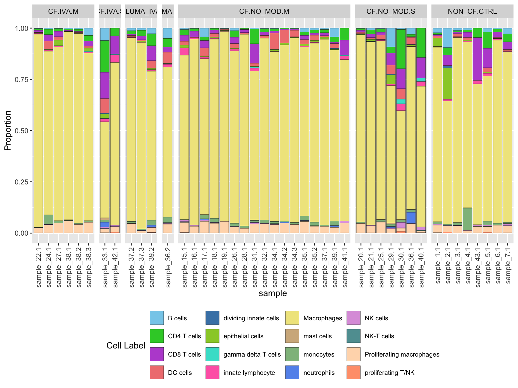

Cell proportions by cell type

props$Proportions %>%
  data.frame %>%
  inner_join(seu@meta.data %>%
               dplyr::select(sample.id,
                             Annotation,
                             Broad,
                             Disease,
                             Treatment,
                             Status, 
                             Severity, 
                             Batch, 
                             Age, 
                             Sex), 
             by = c("sample" = "sample.id", "clusters" = "Broad")) %>%
  distinct()-> dat

ggplot(dat, 
       aes(x = clusters, y = Freq, fill = clusters)) +
  geom_boxplot(outlier.size = 0.1, size = 0.25) +
  theme(axis.text.x = element_text(angle = 45,
                                   vjust = 1,
                                   hjust = 1),
        legend.text = element_text(size = 8)) +
  labs(y = "Proportion") +
  scale_fill_paletteer_d("miscpalettes::pastel", direction = 1) +
  NoLegend()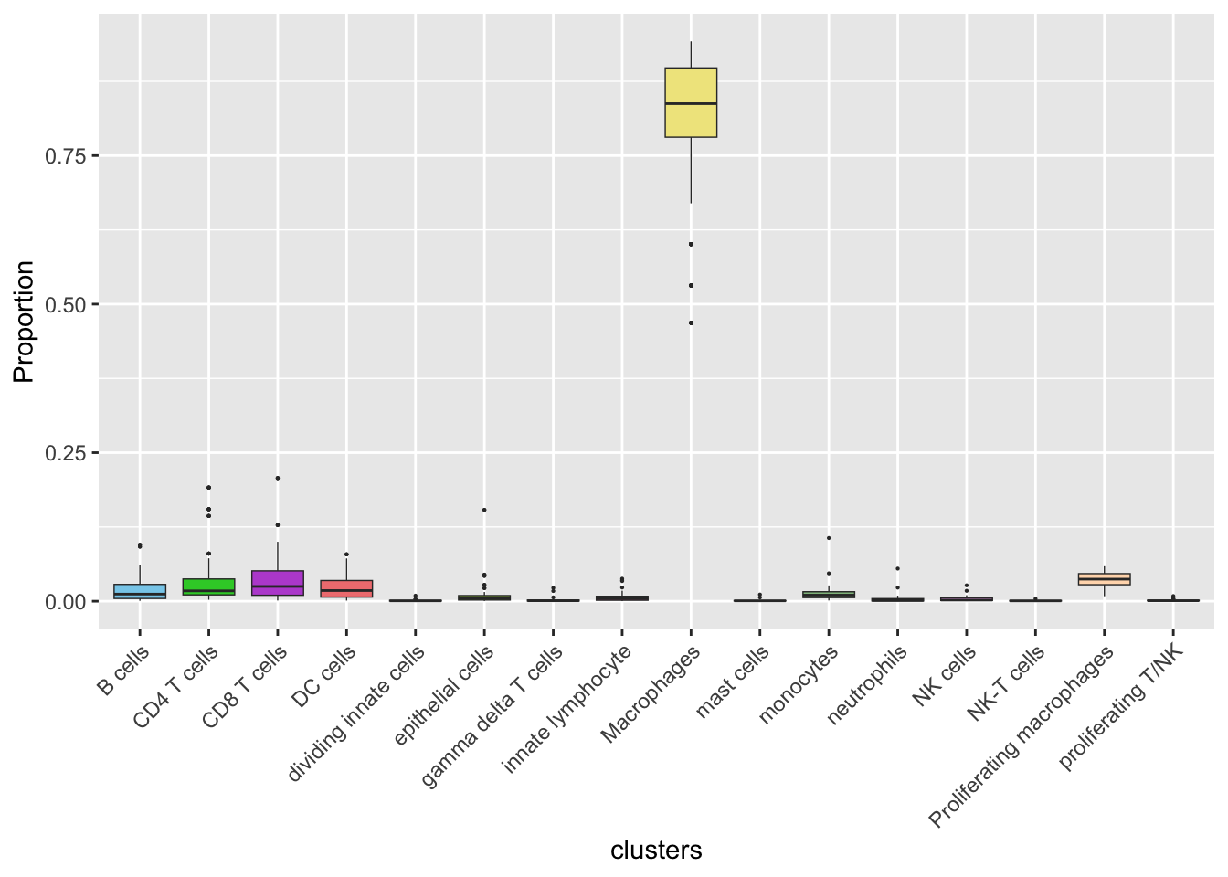

Explore sources of variation

Cell count data

Look at the sources of variation in the raw cell count level data.

dims <- list(c(1,2), c(2:3), c(3,4), c(4,5))
p <- vector("list", length(dims))

for(i in 1:length(dims)){
  mds <- plotMDS(props$Counts,
    gene.selection = "common",
    plot = FALSE, dim.plot = dims[[i]])
  
  data.frame(x = mds$x, 
             y = mds$y,
             sample = rownames(mds$distance.matrix.squared)) %>%
    left_join(seu@meta.data %>%
               dplyr::select(sample.id, 
                             Disease,
                             Treatment,
                             Status, 
                             Severity, 
                             Batch, 
                             Age, 
                             Sex), 
             by = c("sample" = "sample.id")) %>%
    distinct() -> dat
  
  p[[i]] <- ggplot(dat, aes(x = x, y = y, 
                            shape = as.factor(Disease),
                            color = as.factor(Batch))) +
    geom_point(size = 3) +
    labs(x = glue("Principal Component {dims[[i]][1]}"),
         y = glue("Principal Component {dims[[i]][2]}"),
         colour = "Batch",
         shape = "Disease") +
    theme(legend.direction = "horizontal",
          legend.text = element_text(size = 8),
          legend.title = element_text(size = 9),
          axis.text = element_text(size = 8),
          axis.title = element_text(size = 9)) 
}

wrap_plots(p, cols = 2) + plot_layout(guides = "collect") &
  theme(legend.position = "bottom")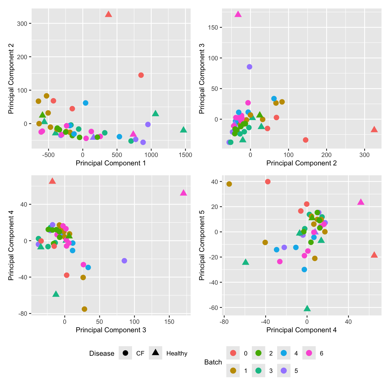

dims <- list(c(1,2), c(2:3), c(3,4), c(4,5))
p <- vector("list", length(dims))

for(i in 1:length(dims)){
  mds <- plotMDS(props$Counts, 
                 gene.selection = "common",
                 plot = FALSE, dim.plot = dims[[i]])
  
   data.frame(x = mds$x, 
             y = mds$y,
             sample = rownames(mds$distance.matrix.squared)) %>%
    left_join(seu@meta.data %>%
               dplyr::select(sample.id, 
                             Disease,
                             Treatment,
                             Status, 
                             Severity,
                             Participant,
                             Batch, 
                             Age, 
                             Sex), 
             by = c("sample" = "sample.id")) %>%
    group_by(sample) %>%
    mutate(ncells = n()) %>%
    ungroup() %>%
    distinct() -> dat
  
  p[[i]] <- ggplot(dat, aes(x = x, y = y, 
                            colour = log2(ncells)))+
    geom_text(aes(label = str_remove_all(sample, "sample_")), size = 2.5) +
    labs(x = glue("Principal Component {dims[[i]][1]}"),
         y = glue("Principal Component {dims[[i]][2]}"),
         colour = "Log2 No. Cells") +
    theme(legend.direction = "horizontal",
          legend.text = element_text(size = 8),
          legend.title = element_text(size = 9),
          axis.text = element_text(size = 8),
          axis.title = element_text(size = 9)) +
    scale_colour_viridis_c(option = "magma")
}

wrap_plots(p, cols = 2) + plot_layout(guides = "collect") &
  theme(legend.position = "bottom")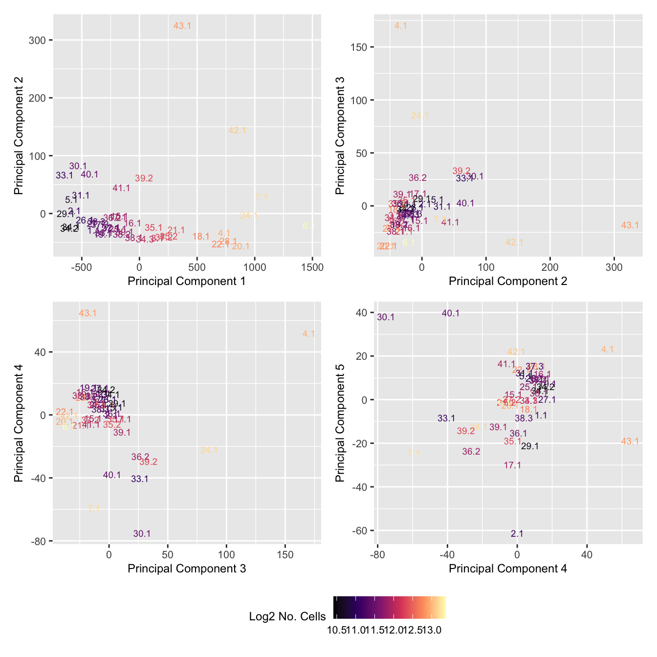

Cell proportion data

Look at the sources of variation in the cell proportions data.

dims <- list(c(1,2), c(2:3), c(3,4), c(4,5))
p <- vector("list", length(dims))

for(i in 1:length(dims)){
  mds <- plotMDS(props$TransformedProps,
    gene.selection = "common",
    plot = FALSE, dim.plot = dims[[i]])
  
  data.frame(x = mds$x, 
             y = mds$y,
             sample = rownames(mds$distance.matrix.squared)) %>%
    left_join(seu@meta.data %>%
               dplyr::select(sample.id, 
                             Disease,
                             Treatment,
                             Status, 
                             Severity, 
                             Batch, 
                             Age, 
                             Sex), 
             by = c("sample" = "sample.id")) %>%
    distinct() -> dat
  
  p[[i]] <- ggplot(dat, aes(x = x, y = y, 
                            shape = as.factor(Disease),
                            color = as.factor(Batch)))+
    geom_point(size = 3) +
    labs(x = glue("Principal Component {dims[[i]][1]}"),
         y = glue("Principal Component {dims[[i]][2]}"),
         colour = "Batch",
         shape = "Disease") +
    theme(legend.direction = "horizontal",
          legend.text = element_text(size = 8),
          legend.title = element_text(size = 9),
          axis.text = element_text(size = 8),
          axis.title = element_text(size = 9))
}

wrap_plots(p, cols = 2) + plot_layout(guides = "collect") &
  theme(legend.position = "bottom")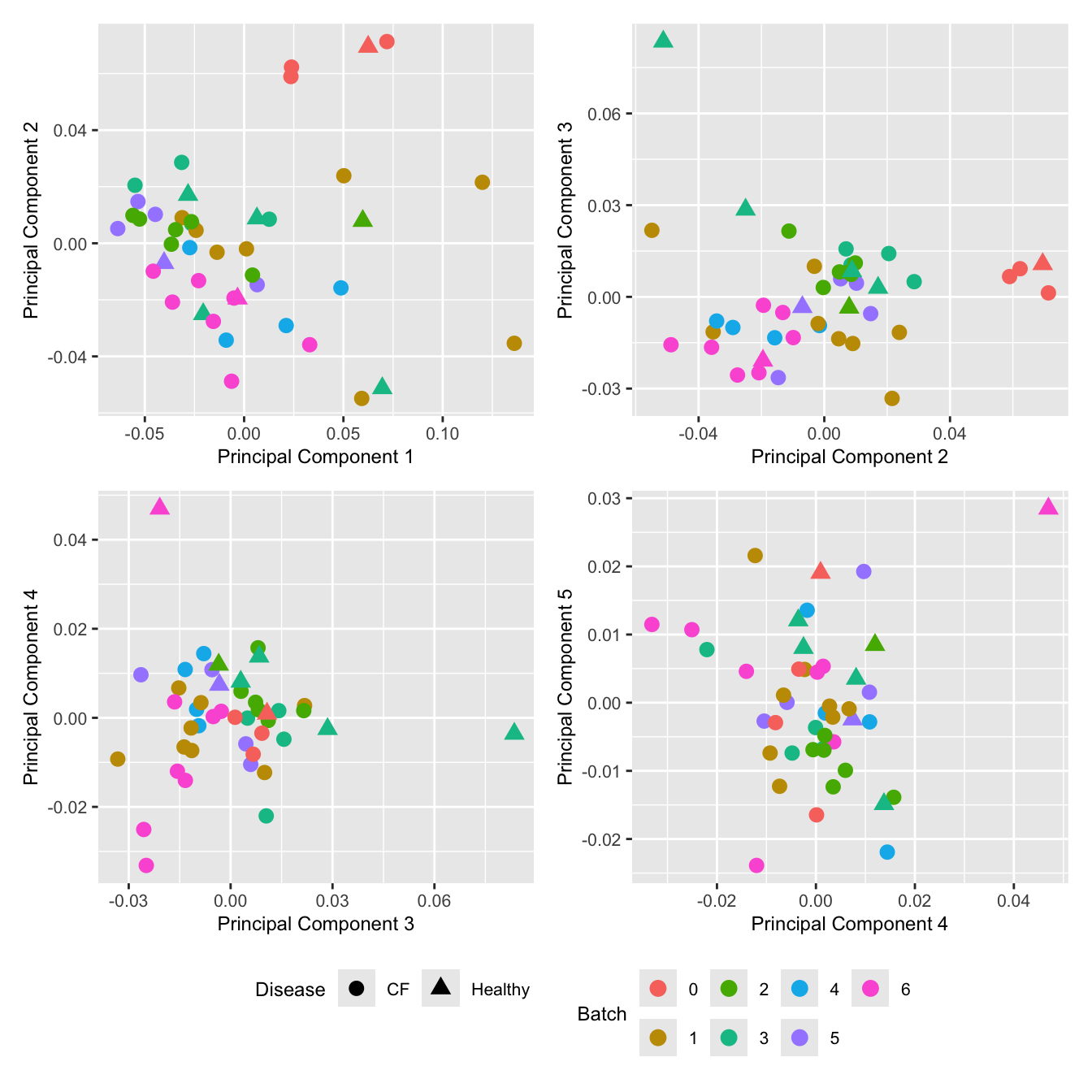

dims <- list(c(1,2), c(2:3), c(3,4), c(4,5))
p <- vector("list", length(dims))

for(i in 1:length(dims)){
  mds <- plotMDS(props$TransformedProps,
    gene.selection = "common",
    plot = FALSE, dim.plot = dims[[i]])
  
  data.frame(x = mds$x, 
             y = mds$y,
             sample = rownames(mds$distance.matrix.squared)) %>%
    left_join(seu@meta.data %>%
               dplyr::select(sample.id, 
                             Disease,
                             Treatment,
                             Status, 
                             Severity, 
                             Batch, 
                             Age, 
                             Sex), 
             by = c("sample" = "sample.id")) %>%
    distinct() -> dat
  
  p[[i]] <- ggplot(dat, aes(x = x, y = y, 
                            shape = as.factor(Disease),
                            color = Sex))+
    geom_point(size = 3) +
    labs(x = glue("Principal Component {dims[[i]][1]}"),
         y = glue("Principal Component {dims[[i]][2]}"),
         colour = "Sex",
         shape = "Disease") +
    theme(legend.direction = "horizontal",
          legend.text = element_text(size = 8),
          legend.title = element_text(size = 9),
          axis.text = element_text(size = 8),
          axis.title = element_text(size = 9))
}

wrap_plots(p, cols = 2) + plot_layout(guides = "collect") &
  theme(legend.position = "bottom")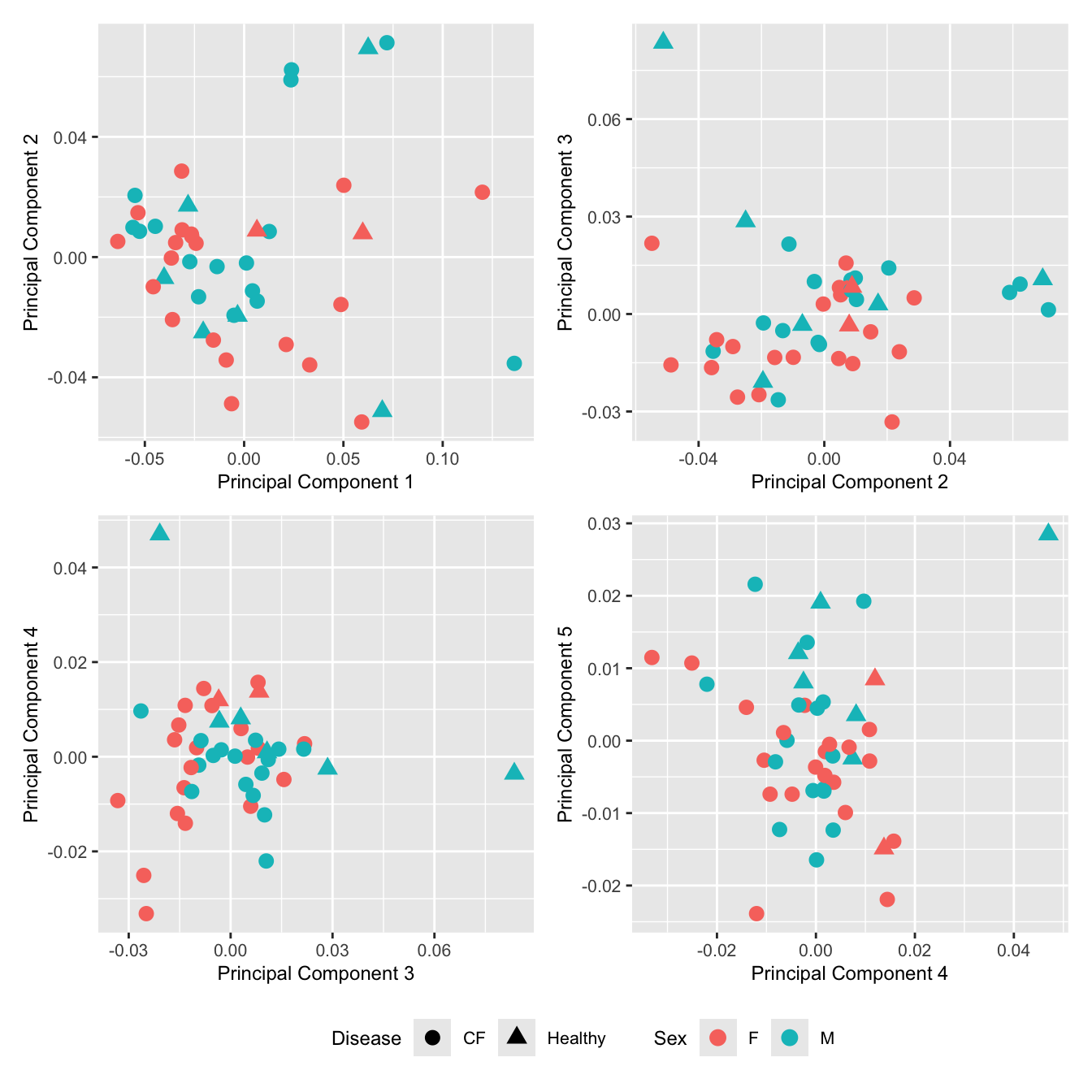

dims <- list(c(1,2), c(2:3), c(3,4), c(4,5))
p <- vector("list", length(dims))

for(i in 1:length(dims)){
  mds <- plotMDS(props$TransformedProps, 
                 gene.selection = "common",
                 plot = FALSE, dim.plot = dims[[i]])
  
   data.frame(x = mds$x, 
             y = mds$y,
             sample = rownames(mds$distance.matrix.squared)) %>%
    left_join(seu@meta.data %>%
               dplyr::select(sample.id, 
                             Disease,
                             Treatment,
                             Status, 
                             Severity,
                             Participant,
                             Batch, 
                             Age, 
                             Sex), 
             by = c("sample" = "sample.id")) %>%
    group_by(sample) %>%
    mutate(ncells = n()) %>%
    ungroup() %>%
    distinct() -> dat
  
  p[[i]] <- ggplot(dat, aes(x = x, y = y, 
                            colour = log2(Age)))+
    geom_text(aes(label = str_remove_all(sample, "sample_")), size = 2.5) +
    labs(x = glue("Principal Component {dims[[i]][1]}"),
         y = glue("Principal Component {dims[[i]][2]}"),
         colour = "Log2 Age") +
    theme(legend.direction = "horizontal",
          legend.text = element_text(size = 8),
          legend.title = element_text(size = 9),
          axis.text = element_text(size = 8),
          axis.title = element_text(size = 9)) +
    scale_colour_viridis_c(option = "magma")
}

wrap_plots(p, cols = 2) + plot_layout(guides = "collect") &
  theme(legend.position = "bottom")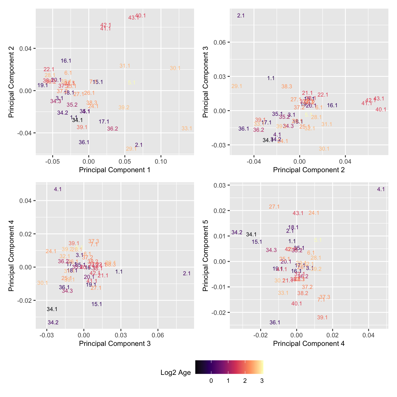

dims <- list(c(1,2), c(2:3), c(3,4), c(4,5))
p <- vector("list", length(dims))

for(i in 1:length(dims)){
  mds <- plotMDS(props$TransformedProps, 
                 gene.selection = "common",
                 plot = FALSE, dim.plot = dims[[i]])
  
   data.frame(x = mds$x, 
             y = mds$y,
             sample = rownames(mds$distance.matrix.squared)) %>%
    left_join(seu@meta.data %>%
               dplyr::select(sample.id, 
                             Disease,
                             Treatment,
                             Status, 
                             Severity,
                             Participant,
                             Batch, 
                             Age, 
                             Sex), 
             by = c("sample" = "sample.id")) %>%
    group_by(sample) %>%
    mutate(ncells = n()) %>%
    ungroup() %>%
    distinct() -> dat
  
  p[[i]] <- ggplot(dat, aes(x = x, y = y, 
                            colour = log2(ncells)))+
    geom_text(aes(label = str_remove_all(sample, "sample_")), size = 2.5) +
    labs(x = glue("Principal Component {dims[[i]][1]}"),
         y = glue("Principal Component {dims[[i]][2]}"),
         colour = "Log2 No. Cells") +
    theme(legend.direction = "horizontal",
          legend.text = element_text(size = 8),
          legend.title = element_text(size = 9),
          axis.text = element_text(size = 8),
          axis.title = element_text(size = 9)) +
    scale_colour_viridis_c(option = "magma")
}

wrap_plots(p, cols = 2) + plot_layout(guides = "collect") &
  theme(legend.position = "bottom")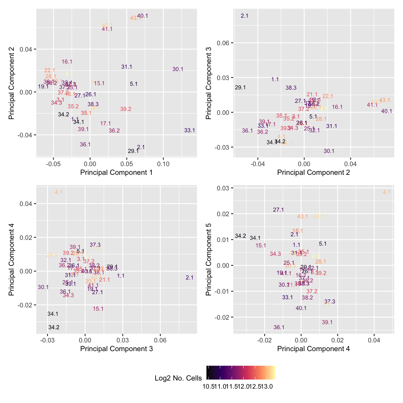

Principal components versus traits

Principal components analysis (PCA) allows us to mathematically determine the sources of variation in the data. We can then investigate whether these correlate with any of the specifed covariates. First, we calculate the principal components. The scree plot belows shows us that most of the variation in this data is captured by the top 7 principal components.

PCs <- prcomp(t(props$TransformedProps), center = TRUE, 
              scale = TRUE, retx = TRUE)
loadings = PCs$x # pc loadings
plot(PCs, type="lines") # scree plot

Collect all of the known sample traits.

nGenes = nrow(props$TransformedProps)
nSamples = ncol(props$TransformedProps)

info <- seu@meta.data %>%
  dplyr::select(sample.id, 
                Disease,
                Treatment,
                Status, 
                Severity,
                Participant,
                Group,
                Batch, 
                Age, 
                Sex) %>%
  group_by(sample.id) %>%
  mutate(ncells = n()) %>%
  ungroup() %>%
  distinct()

m <- match(colnames(props$TransformedProps), info$sample.id)
info <- info[m,]

datTraits <- info %>% dplyr::select(Participant, Batch, Disease, Status,
                                    Group, Severity, Age, Sex, ncells) %>%
  mutate(Age = log2(Age),
         ncells = log2(ncells),
    Donor = factor(Participant),
         Batch = factor(Batch),
         Disease = factor(Disease, 
                          labels = 1:length(unique(Disease))),
         Group = factor(Group, 
                        labels = 1:length(unique(Group))),
         Treatment = factor(Status, 
                            labels = 1:length(unique(Status))),
         Sex = factor(Sex, labels = length(unique(Sex))),
         Severity = factor(Severity, labels = length(unique(Severity)))) %>%
  mutate(across(everything(), as.numeric)) %>%
  dplyr::select(-Participant, -Status)

datTraits %>% 
  knitr::kable()

Batch	Disease	Group	Severity	Age	Sex	ncells	Donor	Treatment
4	2	7	1	-0.2590872	2	11.21006	1	4
4	1	5	2	-0.0939001	2	11.82416	2	3
4	1	5	2	-0.1151479	1	11.85604	3	3
5	1	5	2	-0.0441471	1	11.86573	4	3
5	1	5	2	0.1428834	2	12.68036	5	3
6	1	5	2	-0.0729608	1	11.29577	6	3
4	2	7	1	0.1464588	2	11.13635	7	4
6	1	6	3	0.5597097	2	12.93055	8	3
4	1	6	3	1.5743836	1	12.41627	9	3
4	1	1	2	1.5993830	2	12.73640	10	1
6	1	1	2	2.3883594	2	13.17633	11	1
2	1	6	3	2.2957230	1	11.67596	12	3
2	1	5	2	2.3360877	2	10.99435	13	3
2	1	1	2	2.2980155	2	11.26854	14	1
6	1	5	2	2.5790214	1	12.80554	15	3
2	1	6	3	2.5823250	1	10.61471	16	3
6	2	7	1	0.1321035	2	12.19414	17	4
2	1	6	3	2.5889097	1	11.43671	18	3
2	1	5	2	2.5583683	1	11.07682	19	3
2	1	5	2	2.5670653	1	11.53284	20	3
2	1	2	3	2.5730557	2	11.06272	21	1
7	1	5	2	-0.9343238	1	10.54689	22	3
7	1	5	2	0.0918737	1	10.41680	22	3
7	1	5	2	1.0409164	1	12.04337	22	3
7	1	5	2	0.0807044	2	12.27612	23	3
7	1	5	2	0.9940589	2	12.36987	23	3
7	1	6	3	-0.0564254	1	11.54448	24	3
7	1	4	3	1.1764977	1	11.82217	24	2
3	1	5	2	1.5597097	1	11.48884	25	3
3	1	3	2	2.1930156	1	12.27816	25	2
3	1	3	2	2.2980155	1	11.26562	25	2
3	1	1	2	1.5703964	2	11.86147	26	1
3	1	1	2	2.0206033	2	11.65821	26	1
3	1	1	2	2.3485584	2	11.33483	26	1
5	1	5	2	1.9730702	1	11.85565	27	3
5	1	3	2	2.6297159	1	12.33371	27	2
7	2	7	1	0.2923784	2	12.97782	28	4
1	1	6	3	1.5801455	2	11.41996	29	3
1	1	5	2	1.5801455	2	11.88417	30	3
1	1	2	3	1.5993178	2	13.10214	31	1
1	2	7	1	1.5849625	2	12.84333	32	4
3	2	7	1	3.0699187	1	10.78054	33	4
4	2	7	1	2.4204621	2	13.37246	34	4
4	2	7	1	2.2356012	1	13.20075	35	4

Correlate known sample traits with the top 10 principal components. This can help us determine which traits are potentially contributing to the main sources of variation in the data and should thus be included in our statistical analysis.

moduleTraitCor <- suppressWarnings(cor(loadings[, 1:10], datTraits, use = "p"))
moduleTraitPvalue <- WGCNA::corPvalueStudent(moduleTraitCor, (nSamples - 2))

textMatrix <- paste(signif(moduleTraitCor, 2), "\n(", 
                    signif(moduleTraitPvalue, 1), ")", sep = "")
dim(textMatrix) <- dim(moduleTraitCor)

## Display the correlation values within a heatmap plot
par(cex=0.75, mar = c(6, 8.5, 3, 3))
WGCNA::labeledHeatmap(Matrix = t(moduleTraitCor),
                      xLabels = colnames(loadings)[1:10],
                      yLabels = names(datTraits),
                      colorLabels = FALSE,
                      colors = WGCNA::blueWhiteRed(6),
                      textMatrix = t(textMatrix),
                      setStdMargins = FALSE,
                      cex.text = 1,
                      zlim = c(-1,1),
                      main = paste("PCA-trait relationships: Top 10 PCs"))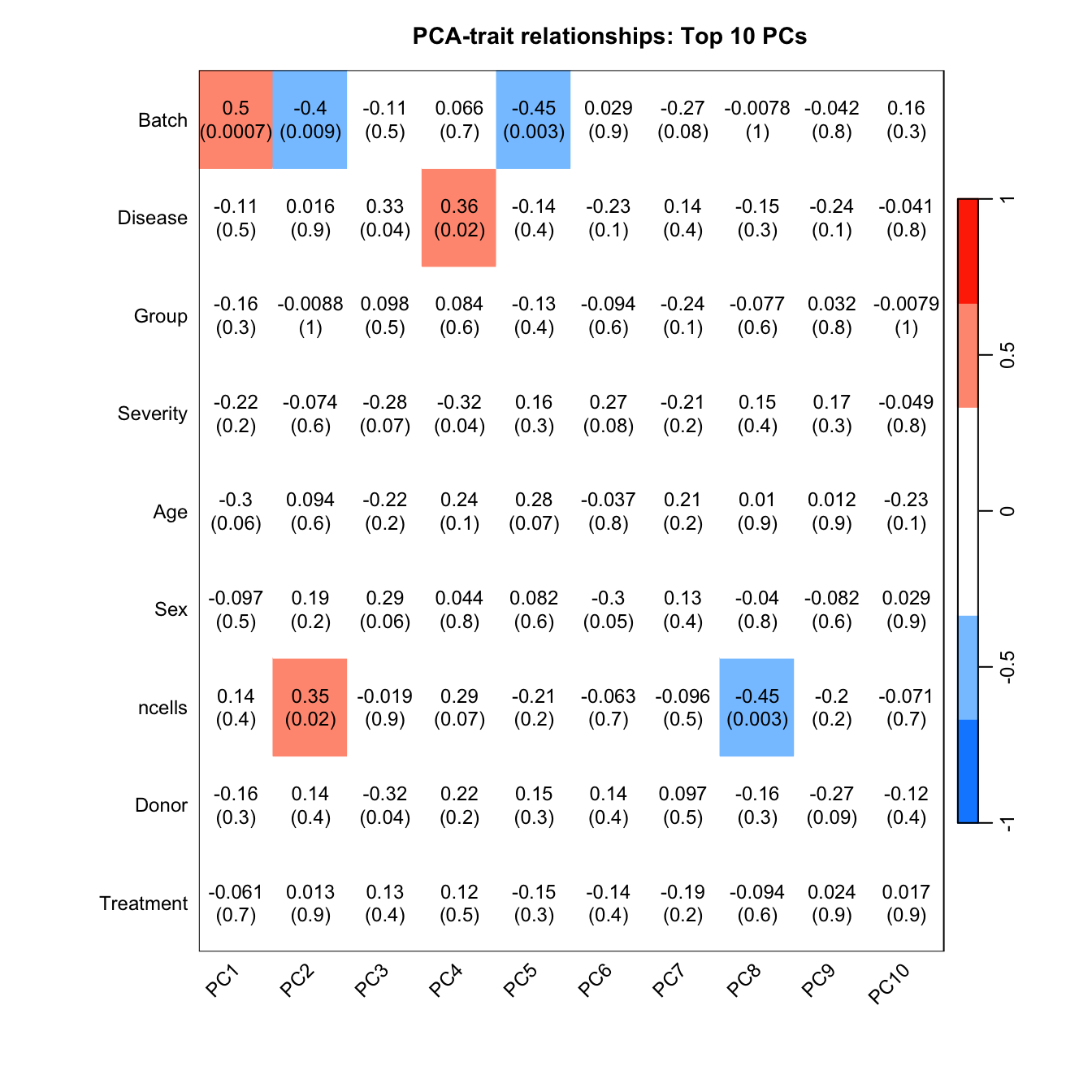

Statistical analysis using the `propeller` and `limma` approach

Create the design matrix.

group <- factor(info$Group)
participant <- factor(info$Participant)
age <- log2(info$Age)
batch <- factor(info$Batch)
sex <- factor(info$Sex)

design <- model.matrix(~ 0 + group + batch)
colnames(design)[1:7] <- levels(group) 
design

   CF.IVA.M CF.IVA.S CF.LUMA_IVA.M CF.LUMA_IVA.S CF.NO_MOD.M CF.NO_MOD.S
1         0        0             0             0           0           0
2         0        0             0             0           1           0
3         0        0             0             0           1           0
4         0        0             0             0           1           0
5         0        0             0             0           1           0
6         0        0             0             0           1           0
7         0        0             0             0           0           0
8         0        0             0             0           0           1
9         0        0             0             0           0           1
10        1        0             0             0           0           0
11        1        0             0             0           0           0
12        0        0             0             0           0           1
13        0        0             0             0           1           0
14        1        0             0             0           0           0
15        0        0             0             0           1           0
16        0        0             0             0           0           1
17        0        0             0             0           0           0
18        0        0             0             0           0           1
19        0        0             0             0           1           0
20        0        0             0             0           1           0
21        0        1             0             0           0           0
22        0        0             0             0           1           0
23        0        0             0             0           1           0
24        0        0             0             0           1           0
25        0        0             0             0           1           0
26        0        0             0             0           1           0
27        0        0             0             0           0           1
28        0        0             0             1           0           0
29        0        0             0             0           1           0
30        0        0             1             0           0           0
31        0        0             1             0           0           0
32        1        0             0             0           0           0
33        1        0             0             0           0           0
34        1        0             0             0           0           0
35        0        0             0             0           1           0
36        0        0             1             0           0           0
37        0        0             0             0           0           0
38        0        0             0             0           0           1
39        0        0             0             0           1           0
40        0        1             0             0           0           0
41        0        0             0             0           0           0
42        0        0             0             0           0           0
43        0        0             0             0           0           0
44        0        0             0             0           0           0
   NON_CF.CTRL batch1 batch2 batch3 batch4 batch5 batch6
1            1      0      0      1      0      0      0
2            0      0      0      1      0      0      0
3            0      0      0      1      0      0      0
4            0      0      0      0      1      0      0
5            0      0      0      0      1      0      0
6            0      0      0      0      0      1      0
7            1      0      0      1      0      0      0
8            0      0      0      0      0      1      0
9            0      0      0      1      0      0      0
10           0      0      0      1      0      0      0
11           0      0      0      0      0      1      0
12           0      1      0      0      0      0      0
13           0      1      0      0      0      0      0
14           0      1      0      0      0      0      0
15           0      0      0      0      0      1      0
16           0      1      0      0      0      0      0
17           1      0      0      0      0      1      0
18           0      1      0      0      0      0      0
19           0      1      0      0      0      0      0
20           0      1      0      0      0      0      0
21           0      1      0      0      0      0      0
22           0      0      0      0      0      0      1
23           0      0      0      0      0      0      1
24           0      0      0      0      0      0      1
25           0      0      0      0      0      0      1
26           0      0      0      0      0      0      1
27           0      0      0      0      0      0      1
28           0      0      0      0      0      0      1
29           0      0      1      0      0      0      0
30           0      0      1      0      0      0      0
31           0      0      1      0      0      0      0
32           0      0      1      0      0      0      0
33           0      0      1      0      0      0      0
34           0      0      1      0      0      0      0
35           0      0      0      0      1      0      0
36           0      0      0      0      1      0      0
37           1      0      0      0      0      0      1
38           0      0      0      0      0      0      0
39           0      0      0      0      0      0      0
40           0      0      0      0      0      0      0
41           1      0      0      0      0      0      0
42           1      0      1      0      0      0      0
43           1      0      0      1      0      0      0
44           1      0      0      1      0      0      0
attr(,"assign")
 [1] 1 1 1 1 1 1 1 2 2 2 2 2 2
attr(,"contrasts")
attr(,"contrasts")$group
[1] "contr.treatment"

attr(,"contrasts")$batch
[1] "contr.treatment"

Create the contrast matrix.

contr <- makeContrasts(CF.NO_MODvCF.IVA = 0.5*(CF.NO_MOD.M + CF.NO_MOD.S) - 0.5*(CF.IVA.M + CF.IVA.S),
                       CF.NO_MODvCF.LUMA_IVA = 0.5*(CF.NO_MOD.M + CF.NO_MOD.S) - 0.5*(CF.LUMA_IVA.M + CF.LUMA_IVA.S),
                       CF.NO_MOD.MvCF.NO_MOD.S = CF.NO_MOD.M - CF.NO_MOD.S,
                       CF.NO_MODvNON_CF.CTRL = 0.5*(CF.NO_MOD.M + CF.NO_MOD.S) - NON_CF.CTRL,
                       CF.IVAvNON_CF.CTRL = 0.5*(CF.IVA.M + CF.IVA.S) - NON_CF.CTRL,
                       CF.LUMA_IVAvNON_CF.CTRL = 0.5*(CF.LUMA_IVA.M + CF.LUMA_IVA.S) - NON_CF.CTRL,
                       levels = design)
contr

               Contrasts
Levels          CF.NO_MODvCF.IVA CF.NO_MODvCF.LUMA_IVA CF.NO_MOD.MvCF.NO_MOD.S
  CF.IVA.M                  -0.5                   0.0                       0
  CF.IVA.S                  -0.5                   0.0                       0
  CF.LUMA_IVA.M              0.0                  -0.5                       0
  CF.LUMA_IVA.S              0.0                  -0.5                       0
  CF.NO_MOD.M                0.5                   0.5                       1
  CF.NO_MOD.S                0.5                   0.5                      -1
  NON_CF.CTRL                0.0                   0.0                       0
  batch1                     0.0                   0.0                       0
  batch2                     0.0                   0.0                       0
  batch3                     0.0                   0.0                       0
  batch4                     0.0                   0.0                       0
  batch5                     0.0                   0.0                       0
  batch6                     0.0                   0.0                       0
               Contrasts
Levels          CF.NO_MODvNON_CF.CTRL CF.IVAvNON_CF.CTRL
  CF.IVA.M                        0.0                0.5
  CF.IVA.S                        0.0                0.5
  CF.LUMA_IVA.M                   0.0                0.0
  CF.LUMA_IVA.S                   0.0                0.0
  CF.NO_MOD.M                     0.5                0.0
  CF.NO_MOD.S                     0.5                0.0
  NON_CF.CTRL                    -1.0               -1.0
  batch1                          0.0                0.0
  batch2                          0.0                0.0
  batch3                          0.0                0.0
  batch4                          0.0                0.0
  batch5                          0.0                0.0
  batch6                          0.0                0.0
               Contrasts
Levels          CF.LUMA_IVAvNON_CF.CTRL
  CF.IVA.M                          0.0
  CF.IVA.S                          0.0
  CF.LUMA_IVA.M                     0.5
  CF.LUMA_IVA.S                     0.5
  CF.NO_MOD.M                       0.0
  CF.NO_MOD.S                       0.0
  NON_CF.CTRL                      -1.0
  batch1                            0.0
  batch2                            0.0
  batch3                            0.0
  batch4                            0.0
  batch5                            0.0
  batch6                            0.0

Add random effect for samples from the same individual.

dupcor <- duplicateCorrelation(props$TransformedProps, design=design,
                                block=participant)
dupcor

$consensus.correlation
[1] 0.6475815

$cor
[1] 0.6475815

$atanh.correlations
 [1]  0.7046178  1.2192721  0.3225704  0.5734219  0.3836834  1.2106267
 [7]  0.1105819  1.0992546  0.8331586  0.4470538  1.7268879  1.5298445
[13]  0.9810777  0.6771234 -0.5360603  0.8016052

Fit the model.

fit <- lmFit(props$TransformedProps, design=design, block=participant, 
                correlation=dupcor$consensus)
fit2 <- contrasts.fit(fit, contr)
fit2 <- eBayes(fit2, robust=TRUE, trend=FALSE)
pvalue <- 0.05
summary(decideTests(fit2, p.value = pvalue))

       CF.NO_MODvCF.IVA CF.NO_MODvCF.LUMA_IVA CF.NO_MOD.MvCF.NO_MOD.S
Down                  0                     0                       0
NotSig               16                    15                      16
Up                    0                     1                       0
       CF.NO_MODvNON_CF.CTRL CF.IVAvNON_CF.CTRL CF.LUMA_IVAvNON_CF.CTRL
Down                       1                  0                       0
NotSig                    15                 16                      16
Up                         0                  0                       0

Results

ANOVA

topTable(fit2)

                    CF.NO_MODvCF.IVA CF.NO_MODvCF.LUMA_IVA
neutrophils             -0.019722250            0.06035614
monocytes               -0.024786560           -0.02592302
mast cells              -0.019323905            0.01383322
CD8 T cells             -0.031004443           -0.07544362
Macrophages              0.055336009            0.06147213
innate lymphocyte       -0.012832123           -0.04659819
B cells                 -0.028030487           -0.03594194
CD4 T cells             -0.007798471           -0.06683024
NK cells                 0.009068285           -0.01615113
gamma delta T cells      0.016074104            0.01262772
                    CF.NO_MOD.MvCF.NO_MOD.S CF.NO_MODvNON_CF.CTRL
neutrophils                   -0.0354748540          0.0189455379
monocytes                      0.0003329593         -0.0716913715
mast cells                    -0.0109423278         -0.0091787516
CD8 T cells                   -0.0067822197         -0.0774654928
Macrophages                    0.0865178054          0.0897824139
innate lymphocyte             -0.0035924063         -0.0009096075
B cells                       -0.0525320831         -0.0469602254
CD4 T cells                   -0.0546268729         -0.0081952353
NK cells                      -0.0225312262         -0.0036286783
gamma delta T cells           -0.0232651224          0.0197439955
                    CF.IVAvNON_CF.CTRL CF.LUMA_IVAvNON_CF.CTRL    AveExpr
neutrophils                0.038667788            -0.041410598 0.03225974
monocytes                 -0.046904811            -0.045768351 0.09640016
mast cells                 0.010145153            -0.023011974 0.01581934
CD8 T cells               -0.046461050            -0.002021871 0.16947960
Macrophages                0.034446405             0.028310282 1.14015663
innate lymphocyte          0.011922515             0.045688580 0.07422051
B cells                   -0.018929738            -0.011018281 0.10119310
CD4 T cells               -0.000396764             0.058635003 0.16060800
NK cells                  -0.012696963             0.012522454 0.05126451
gamma delta T cells        0.003669892             0.007116278 0.02480051
                           F     P.Value adj.P.Val
neutrophils         4.781092 0.003701551 0.0316720
monocytes           4.723029 0.003959000 0.0316720
mast cells          2.368124 0.072577232 0.3061273
CD8 T cells         2.329604 0.076531821 0.3061273
Macrophages         1.997970 0.117789623 0.3662978
innate lymphocyte   1.878489 0.137361662 0.3662978
B cells             1.732906 0.166309247 0.3760054
CD4 T cells         1.638400 0.188002704 0.3760054
NK cells            1.105613 0.370196928 0.6157466
gamma delta T cells 1.074179 0.384841613 0.6157466

p <- vector("list", ncol(contr))

for(i in 1:ncol(contr)){
props$Proportions %>% data.frame %>%
  left_join(info,
            by = c("sample" = "sample.id")) %>%
  dplyr::filter(Group %in%  names(contr[, i])[abs(contr[, i]) > 0]) -> dat
  
  if(length(unique(dat$Group)) > 2) dat$Group <- str_remove(dat$Group, ".(M|S)$")
ggplot(dat, aes(x = Group,
                y = Freq,
                colour = Group,
                group = Group)) +
  geom_boxplot(outlier.shape = NA, colour = "grey") +
  geom_jitter(stat = "identity",
              width = 0.15,
              size = 2) +
  theme_classic() +
  theme(axis.text.x = element_text(angle = 90,
                                   hjust = 1,
                                   vjust = 0.5),
        legend.position = "bottom",
        legend.direction = "horizontal") +
  labs(x = "Group", y = "Proportion",
       colour = "Condition") +
  facet_wrap(~clusters, scales = "free_y") -> p[[i]]
}

p

[[1]]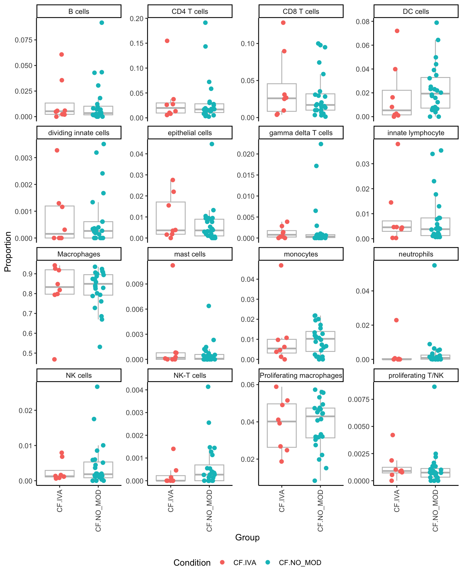


[[2]]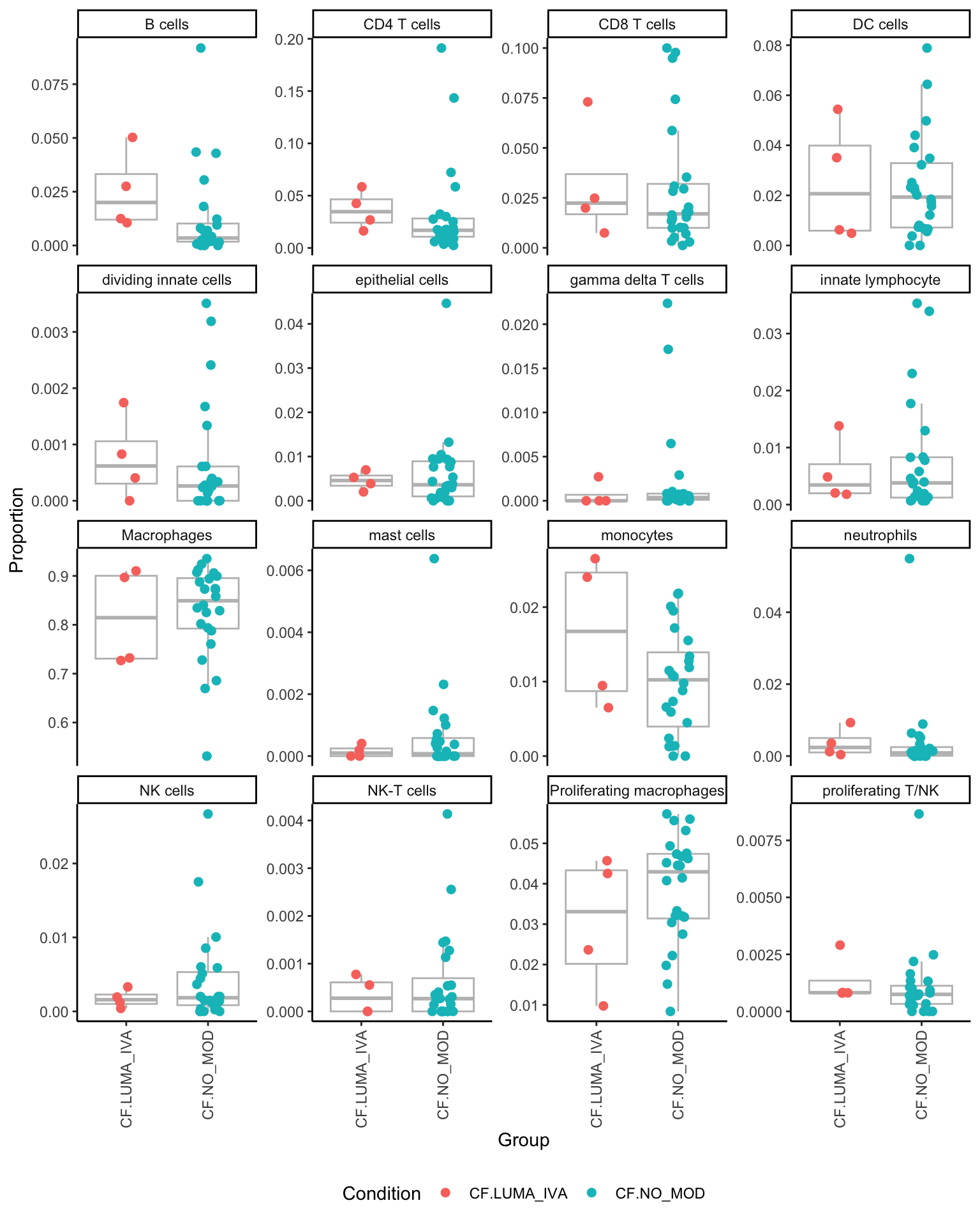


[[3]]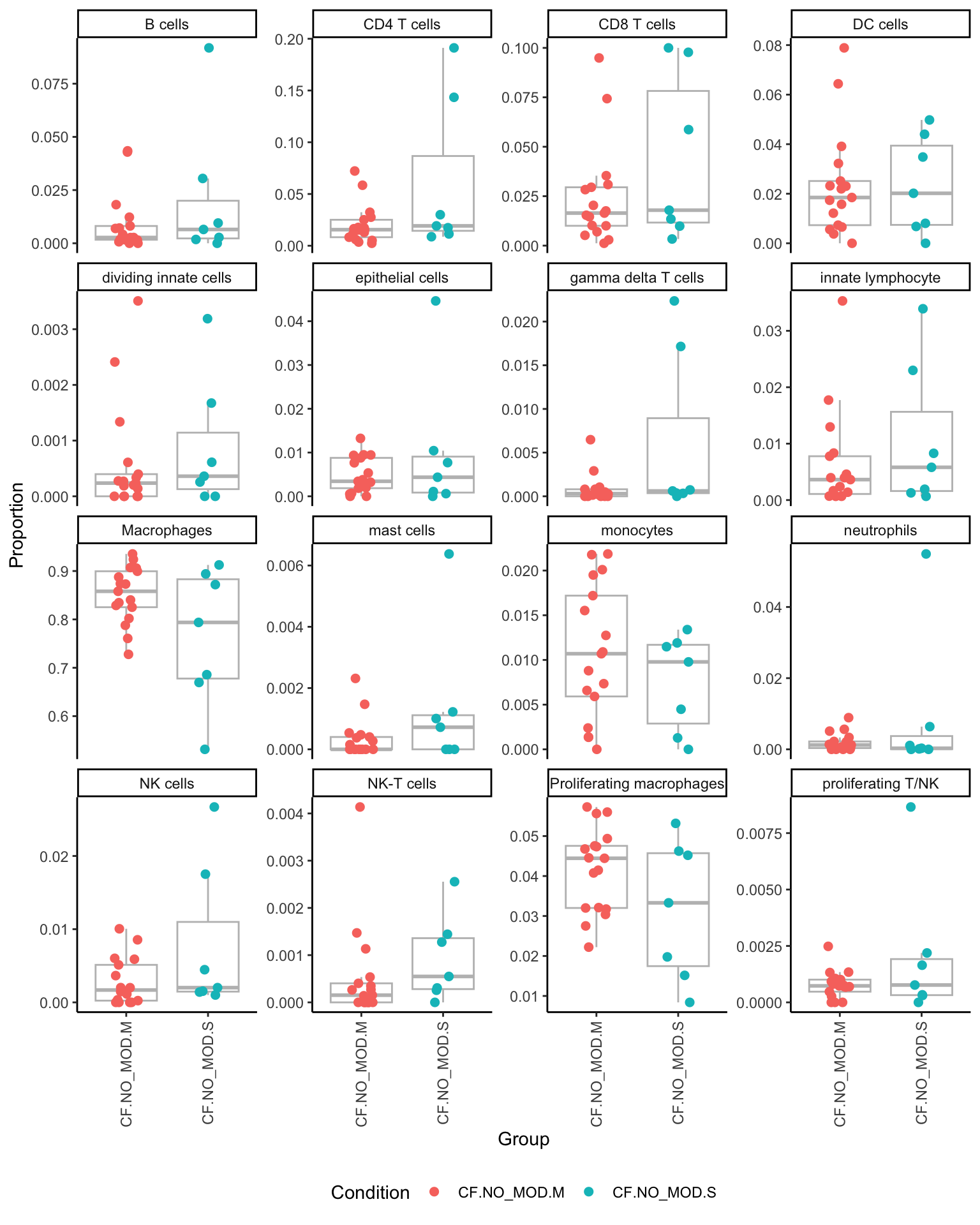


[[4]]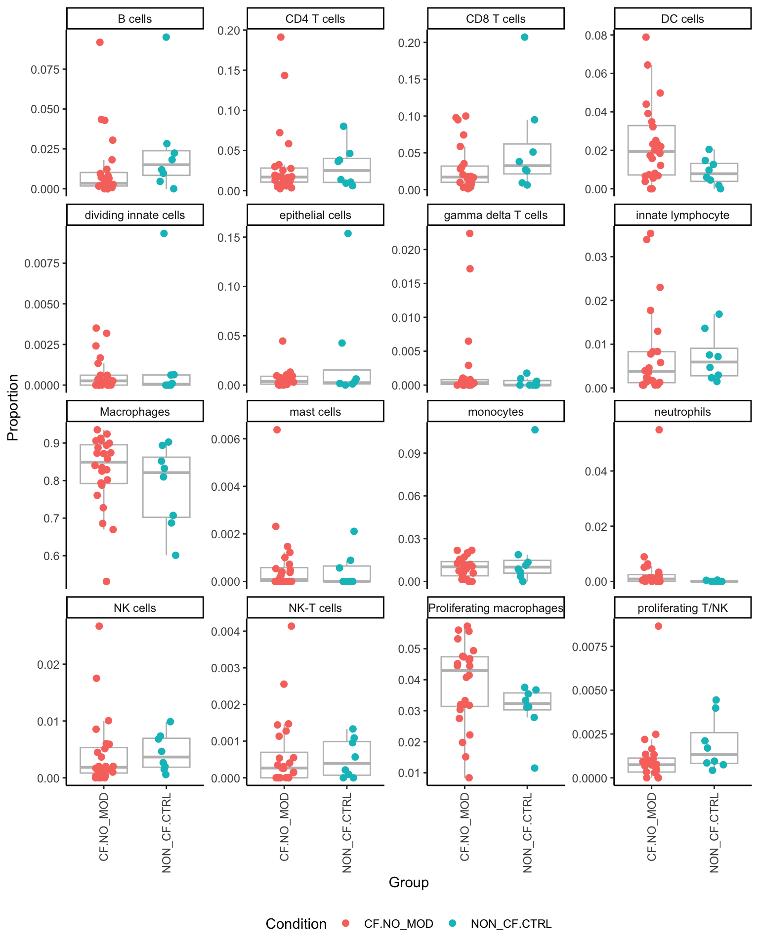


[[5]]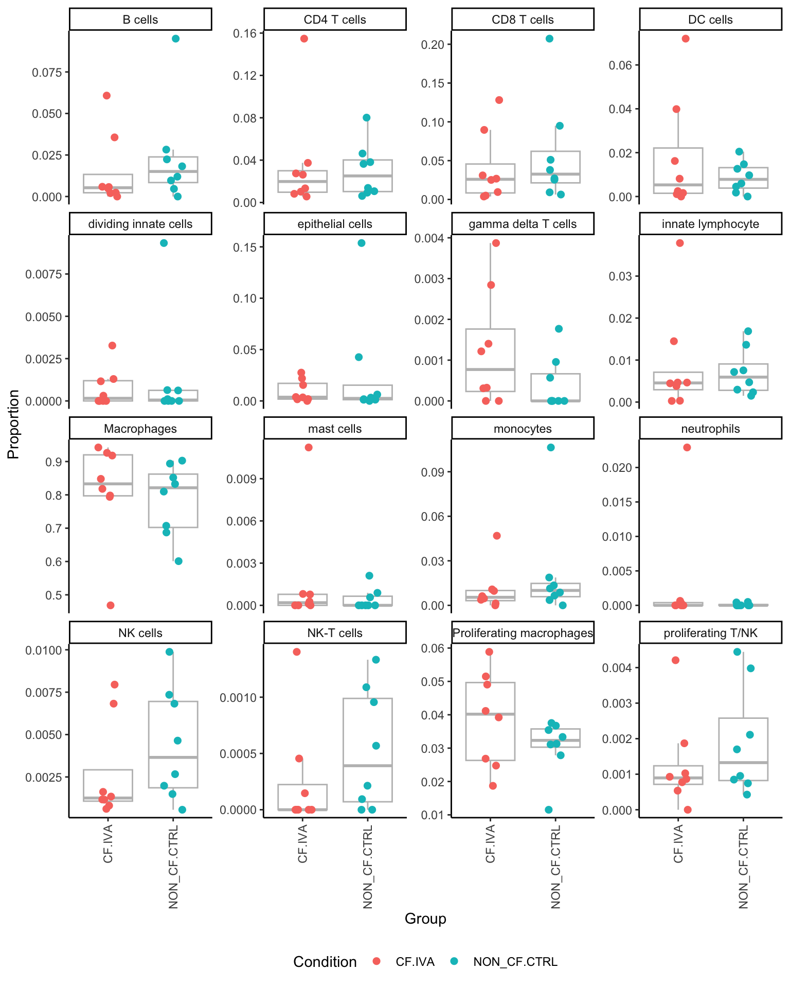


[[6]]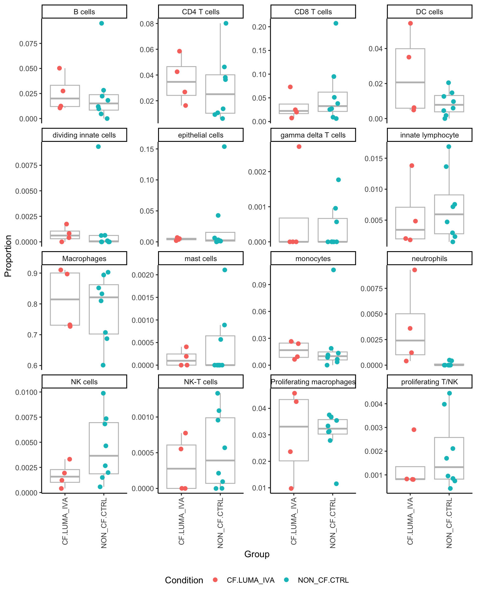

Session info

The analysis and this document were prepared using the following software (click triangle to expand)

sessioninfo::session_info()

─ Session info ───────────────────────────────────────────────────────────────
 setting  value
 version  R version 4.3.2 (2023-10-31)
 os       macOS Sonoma 14.5
 system   aarch64, darwin20
 ui       X11
 language (EN)
 collate  en_US.UTF-8
 ctype    en_US.UTF-8
 tz       Australia/Melbourne
 date     2024-08-09
 pandoc   3.1.11 @ /Applications/RStudio.app/Contents/Resources/app/quarto/bin/tools/aarch64/ (via rmarkdown)

─ Packages ───────────────────────────────────────────────────────────────────
 ! package              * version    date (UTC) lib source
 P abind                  1.4-5      2016-07-21 [?] RSPM (R 4.3.0)
 P AnnotationDbi        * 1.64.1     2023-11-02 [?] Bioconductor
 P backports              1.4.1      2021-12-13 [?] RSPM (R 4.3.0)
 P base64enc              0.1-3      2015-07-28 [?] RSPM (R 4.3.0)
 P Biobase              * 2.62.0     2023-10-26 [?] Bioconductor
 P BiocGenerics         * 0.48.1     2023-11-02 [?] Bioconductor
 P BiocManager            1.30.22    2023-08-08 [?] RSPM (R 4.3.0)
 P Biostrings             2.70.2     2024-01-30 [?] Bioconductor 3.18 (R 4.3.2)
 P bit                    4.0.5      2022-11-15 [?] RSPM (R 4.3.0)
 P bit64                  4.0.5      2020-08-30 [?] RSPM (R 4.3.0)
 P bitops                 1.0-7      2021-04-24 [?] RSPM (R 4.3.0)
 P blob                   1.2.4      2023-03-17 [?] RSPM (R 4.3.0)
 P bslib                  0.6.1      2023-11-28 [?] RSPM (R 4.3.0)
 P cachem                 1.0.8      2023-05-01 [?] RSPM (R 4.3.0)
 P callr                  3.7.3      2022-11-02 [?] RSPM (R 4.3.0)
 P checkmate              2.3.1      2023-12-04 [?] RSPM (R 4.3.0)
 P circlize               0.4.15     2022-05-10 [?] RSPM (R 4.3.0)
 P cli                    3.6.2      2023-12-11 [?] RSPM (R 4.3.0)
 P clue                   0.3-65     2023-09-23 [?] RSPM (R 4.3.0)
 P cluster                2.1.6      2023-12-01 [?] CRAN (R 4.3.1)
 P clustree             * 0.5.1      2023-11-05 [?] RSPM (R 4.3.0)
 P codetools              0.2-20     2024-03-31 [?] CRAN (R 4.3.1)
 P colorspace             2.1-0      2023-01-23 [?] RSPM (R 4.3.0)
 P ComplexHeatmap         2.18.0     2023-10-26 [?] Bioconductor
 P cowplot                1.1.3      2024-01-22 [?] RSPM (R 4.3.0)
 P crayon                 1.5.2      2022-09-29 [?] RSPM (R 4.3.0)
 P data.table             1.15.0     2024-01-30 [?] RSPM (R 4.3.0)
 P DBI                    1.2.1      2024-01-12 [?] RSPM (R 4.3.0)
 P DelayedArray           0.28.0     2023-11-06 [?] Bioconductor
 P deldir                 2.0-2      2023-11-23 [?] RSPM (R 4.3.0)
 P dendextend             1.17.1     2023-03-25 [?] RSPM (R 4.3.0)
 P digest                 0.6.34     2024-01-11 [?] RSPM (R 4.3.0)
 P dittoSeq             * 1.14.2     2024-02-10 [?] Bioconductor 3.18 (R 4.3.2)
 P doParallel             1.0.17     2022-02-07 [?] RSPM (R 4.3.0)
 P dplyr                * 1.1.4      2023-11-17 [?] RSPM (R 4.3.0)
 P dynamicTreeCut         1.63-1     2016-03-11 [?] RSPM (R 4.3.0)
 P edgeR                * 4.0.15     2024-02-10 [?] Bioconductor 3.18 (R 4.3.2)
 P ellipsis               0.3.2      2021-04-29 [?] RSPM (R 4.3.0)
 P evaluate               0.23       2023-11-01 [?] RSPM (R 4.3.0)
 P fansi                  1.0.6      2023-12-08 [?] RSPM (R 4.3.0)
 P farver                 2.1.1      2022-07-06 [?] RSPM (R 4.3.0)
 P fastcluster            1.2.6      2024-01-12 [?] RSPM (R 4.3.0)
 P fastmap                1.1.1      2023-02-24 [?] RSPM (R 4.3.0)
 P fitdistrplus           1.1-11     2023-04-25 [?] RSPM (R 4.3.0)
 P forcats              * 1.0.0      2023-01-29 [?] RSPM (R 4.3.0)
 P foreach                1.5.2      2022-02-02 [?] RSPM (R 4.3.0)
 P foreign                0.8-86     2023-11-28 [?] CRAN (R 4.3.1)
   Formula                1.2-5      2023-02-24 [1] RSPM (R 4.3.0)
 P fs                     1.6.3      2023-07-20 [?] RSPM (R 4.3.0)
 P future                 1.33.1     2023-12-22 [?] RSPM (R 4.3.0)
 P future.apply           1.11.1     2023-12-21 [?] RSPM (R 4.3.0)
 P generics               0.1.3      2022-07-05 [?] RSPM (R 4.3.0)
 P GenomeInfoDb         * 1.38.6     2024-02-10 [?] Bioconductor 3.18 (R 4.3.2)
 P GenomeInfoDbData       1.2.11     2024-02-16 [?] Bioconductor
 P GenomicRanges        * 1.54.1     2023-10-30 [?] Bioconductor
 P GetoptLong             1.0.5      2020-12-15 [?] RSPM (R 4.3.0)
 P getPass                0.2-4      2023-12-10 [?] RSPM (R 4.3.0)
 P ggforce                0.4.2      2024-02-19 [?] RSPM (R 4.3.0)
 P ggplot2              * 3.5.0      2024-02-23 [?] RSPM (R 4.3.0)
 P ggraph               * 2.2.0      2024-02-27 [?] RSPM (R 4.3.0)
 P ggrepel                0.9.5      2024-01-10 [?] RSPM (R 4.3.0)
 P ggridges               0.5.6      2024-01-23 [?] RSPM (R 4.3.0)
 P git2r                  0.33.0     2023-11-26 [?] RSPM (R 4.3.0)
   glmGamPoi            * 1.14.3     2024-02-10 [1] Bioconductor 3.18 (R 4.3.2)
 P GlobalOptions          0.1.2      2020-06-10 [?] RSPM (R 4.3.0)
 P globals                0.16.2     2022-11-21 [?] RSPM (R 4.3.0)
 P glue                 * 1.7.0      2024-01-09 [?] RSPM (R 4.3.0)
 P GO.db                  3.18.0     2024-02-21 [?] Bioconductor
 P goftest                1.2-3      2021-10-07 [?] RSPM (R 4.3.0)
 P graphlayouts           1.1.0      2024-01-19 [?] RSPM (R 4.3.0)
 P gridExtra              2.3        2017-09-09 [?] RSPM (R 4.3.0)
 P gtable                 0.3.4      2023-08-21 [?] RSPM (R 4.3.0)
 P here                 * 1.0.1      2020-12-13 [?] RSPM (R 4.3.0)
 P highr                  0.10       2022-12-22 [?] RSPM (R 4.3.0)
   Hmisc                  5.1-1      2023-09-12 [1] RSPM (R 4.3.0)
 P hms                    1.1.3      2023-03-21 [?] RSPM (R 4.3.0)
   htmlTable              2.4.2      2023-10-29 [1] RSPM (R 4.3.0)
 P htmltools              0.5.7      2023-11-03 [?] RSPM (R 4.3.0)
 P htmlwidgets            1.6.4      2023-12-06 [?] RSPM (R 4.3.0)
 P httpuv                 1.6.14     2024-01-26 [?] RSPM (R 4.3.0)
 P httr                   1.4.7      2023-08-15 [?] RSPM (R 4.3.0)
 P ica                    1.0-3      2022-07-08 [?] RSPM (R 4.3.0)
 P igraph                 2.0.1.1    2024-01-30 [?] RSPM (R 4.3.0)
 P impute                 1.76.0     2023-10-26 [?] Bioconductor
 P IRanges              * 2.36.0     2023-10-26 [?] Bioconductor
 P irlba                  2.3.5.1    2022-10-03 [?] RSPM (R 4.3.0)
 P iterators              1.0.14     2022-02-05 [?] RSPM (R 4.3.0)
 P jquerylib              0.1.4      2021-04-26 [?] RSPM (R 4.3.0)
 P jsonlite               1.8.8      2023-12-04 [?] RSPM (R 4.3.0)
 P KEGGREST               1.42.0     2023-10-26 [?] Bioconductor
 P KernSmooth             2.23-22    2023-07-10 [?] CRAN (R 4.3.2)
 P knitr                  1.45       2023-10-30 [?] RSPM (R 4.3.0)
 P labeling               0.4.3      2023-08-29 [?] RSPM (R 4.3.0)
 P later                  1.3.2      2023-12-06 [?] RSPM (R 4.3.0)
 P lattice                0.22-6     2024-03-20 [?] CRAN (R 4.3.1)
 P lazyeval               0.2.2      2019-03-15 [?] RSPM (R 4.3.0)
 P leiden                 0.4.3.1    2023-11-17 [?] RSPM (R 4.3.0)
 P lifecycle              1.0.4      2023-11-07 [?] RSPM (R 4.3.0)
 P limma                * 3.58.1     2023-11-02 [?] Bioconductor
 P listenv                0.9.1      2024-01-29 [?] RSPM (R 4.3.0)
 P lmtest                 0.9-40     2022-03-21 [?] RSPM (R 4.3.0)
 P locfit                 1.5-9.8    2023-06-11 [?] RSPM (R 4.3.0)
 P lubridate            * 1.9.3      2023-09-27 [?] RSPM (R 4.3.0)
 P magrittr               2.0.3      2022-03-30 [?] RSPM (R 4.3.0)
 P MASS                   7.3-60.0.1 2024-01-13 [?] CRAN (R 4.3.1)
 P Matrix                 1.6-5      2024-01-11 [?] CRAN (R 4.3.1)
 P MatrixGenerics       * 1.14.0     2023-10-26 [?] Bioconductor
 P matrixStats          * 1.2.0      2023-12-11 [?] RSPM (R 4.3.0)
 P memoise                2.0.1      2021-11-26 [?] RSPM (R 4.3.0)
 P mime                   0.12       2021-09-28 [?] RSPM (R 4.3.0)
 P miniUI                 0.1.1.1    2018-05-18 [?] RSPM (R 4.3.0)
 P munsell                0.5.0      2018-06-12 [?] RSPM (R 4.3.0)
 P nlme                   3.1-164    2023-11-27 [?] CRAN (R 4.3.1)
 P nnet                   7.3-19     2023-05-03 [?] CRAN (R 4.3.2)
 P org.Hs.eg.db         * 3.18.0     2024-02-21 [?] Bioconductor
 P paletteer            * 1.6.0      2024-01-21 [?] RSPM (R 4.3.0)
 P parallelly             1.37.0     2024-02-14 [?] RSPM (R 4.3.0)
 P patchwork            * 1.2.0      2024-01-08 [?] RSPM (R 4.3.0)
 P pbapply                1.7-2      2023-06-27 [?] RSPM (R 4.3.0)
 P pheatmap               1.0.12     2019-01-04 [?] RSPM (R 4.3.0)
 P pillar                 1.9.0      2023-03-22 [?] RSPM (R 4.3.0)
 P pkgconfig              2.0.3      2019-09-22 [?] RSPM (R 4.3.0)
 P plotly                 4.10.4     2024-01-13 [?] RSPM (R 4.3.0)
 P plyr                   1.8.9      2023-10-02 [?] RSPM (R 4.3.0)
 P png                    0.1-8      2022-11-29 [?] RSPM (R 4.3.0)
 P polyclip               1.10-6     2023-09-27 [?] RSPM (R 4.3.0)
 P preprocessCore         1.64.0     2023-10-26 [?] Bioconductor
 P prismatic              1.1.1      2022-08-15 [?] RSPM (R 4.3.0)
 P processx               3.8.3      2023-12-10 [?] RSPM (R 4.3.0)
 P progressr              0.14.0     2023-08-10 [?] RSPM (R 4.3.0)
 P promises               1.2.1      2023-08-10 [?] RSPM (R 4.3.0)
 P ps                     1.7.6      2024-01-18 [?] RSPM (R 4.3.0)
 P purrr                * 1.0.2      2023-08-10 [?] RSPM (R 4.3.0)
 P R6                     2.5.1      2021-08-19 [?] RSPM (R 4.3.0)
 P RANN                   2.6.1      2019-01-08 [?] RSPM (R 4.3.0)
 P RColorBrewer           1.1-3      2022-04-03 [?] RSPM (R 4.3.0)
 P Rcpp                   1.0.12     2024-01-09 [?] RSPM (R 4.3.0)
 P RcppAnnoy              0.0.22     2024-01-23 [?] RSPM (R 4.3.0)
 P RCurl                  1.98-1.14  2024-01-09 [?] RSPM (R 4.3.0)
 P readr                * 2.1.5      2024-01-10 [?] RSPM (R 4.3.0)
 P rematch2               2.1.2      2020-05-01 [?] RSPM (R 4.3.0)
   renv                   1.0.3      2023-09-19 [1] CRAN (R 4.3.1)
 P reshape2               1.4.4      2020-04-09 [?] RSPM (R 4.3.0)
 P reticulate             1.35.0     2024-01-31 [?] RSPM (R 4.3.0)
 P rjson                  0.2.21     2022-01-09 [?] RSPM (R 4.3.0)
 P rlang                  1.1.3      2024-01-10 [?] RSPM (R 4.3.0)
 P rmarkdown              2.25       2023-09-18 [?] RSPM (R 4.3.0)
 P ROCR                   1.0-11     2020-05-02 [?] RSPM (R 4.3.0)
 P rpart                  4.1.23     2023-12-05 [?] CRAN (R 4.3.1)
 P rprojroot              2.0.4      2023-11-05 [?] RSPM (R 4.3.0)
 P RSQLite                2.3.5      2024-01-21 [?] RSPM (R 4.3.0)
 P rstudioapi             0.15.0     2023-07-07 [?] RSPM (R 4.3.0)
 P Rtsne                  0.17       2023-12-07 [?] RSPM (R 4.3.0)
 P S4Arrays               1.2.0      2023-10-26 [?] Bioconductor
 P S4Vectors            * 0.40.2     2023-11-25 [?] Bioconductor 3.18 (R 4.3.2)
 P sass                   0.4.8      2023-12-06 [?] RSPM (R 4.3.0)
 P scales                 1.3.0      2023-11-28 [?] RSPM (R 4.3.0)
 P scattermore            1.2        2023-06-12 [?] RSPM (R 4.3.0)
 P sctransform            0.4.1      2023-10-19 [?] RSPM (R 4.3.0)
 P sessioninfo            1.2.2      2021-12-06 [?] RSPM (R 4.3.0)
 P Seurat               * 4.4.0      2023-09-28 [?] RSPM (R 4.3.2)
 P SeuratObject         * 4.1.4      2023-09-26 [?] RSPM (R 4.3.2)
 P shape                  1.4.6      2021-05-19 [?] RSPM (R 4.3.0)
 P shiny                  1.8.0      2023-11-17 [?] RSPM (R 4.3.0)
 P SingleCellExperiment * 1.24.0     2023-11-06 [?] Bioconductor
 P sp                     2.1-3      2024-01-30 [?] RSPM (R 4.3.0)
 P SparseArray            1.2.4      2024-02-10 [?] Bioconductor 3.18 (R 4.3.2)
 P spatstat.data          3.0-4      2024-01-15 [?] RSPM (R 4.3.0)
 P spatstat.explore       3.2-6      2024-02-01 [?] RSPM (R 4.3.0)
 P spatstat.geom          3.2-8      2024-01-26 [?] RSPM (R 4.3.0)
 P spatstat.random        3.2-2      2023-11-29 [?] RSPM (R 4.3.0)
 P spatstat.sparse        3.0-3      2023-10-24 [?] RSPM (R 4.3.0)
 P spatstat.utils         3.0-4      2023-10-24 [?] RSPM (R 4.3.0)
 P speckle              * 1.2.0      2023-10-26 [?] Bioconductor
 P statmod                1.5.0      2023-01-06 [?] RSPM (R 4.3.0)
 P stringi                1.8.3      2023-12-11 [?] RSPM (R 4.3.0)
 P stringr              * 1.5.1      2023-11-14 [?] RSPM (R 4.3.0)
 P SummarizedExperiment * 1.32.0     2023-11-06 [?] Bioconductor
 P survival               3.5-8      2024-02-14 [?] CRAN (R 4.3.1)
 P tensor                 1.5        2012-05-05 [?] RSPM (R 4.3.0)
 P tibble               * 3.2.1      2023-03-20 [?] RSPM (R 4.3.0)
 P tidygraph              1.3.1      2024-01-30 [?] RSPM (R 4.3.0)
 P tidyHeatmap          * 1.8.1      2022-05-20 [?] RSPM (R 4.3.2)
 P tidyr                * 1.3.1      2024-01-24 [?] RSPM (R 4.3.0)
 P tidyselect             1.2.0      2022-10-10 [?] RSPM (R 4.3.0)
 P tidyverse            * 2.0.0      2023-02-22 [?] RSPM (R 4.3.0)
 P timechange             0.3.0      2024-01-18 [?] RSPM (R 4.3.0)
 P tweenr                 2.0.3      2024-02-26 [?] RSPM (R 4.3.0)
 P tzdb                   0.4.0      2023-05-12 [?] RSPM (R 4.3.0)
 P utf8                   1.2.4      2023-10-22 [?] RSPM (R 4.3.0)
 P uwot                   0.1.16     2023-06-29 [?] RSPM (R 4.3.0)
 P vctrs                  0.6.5      2023-12-01 [?] RSPM (R 4.3.0)
 P viridis                0.6.5      2024-01-29 [?] RSPM (R 4.3.0)
 P viridisLite            0.4.2      2023-05-02 [?] RSPM (R 4.3.0)
 P WGCNA                  1.72-5     2023-12-07 [?] RSPM (R 4.3.2)
 P whisker                0.4.1      2022-12-05 [?] RSPM (R 4.3.0)
 P withr                  3.0.0      2024-01-16 [?] RSPM (R 4.3.0)
 P workflowr            * 1.7.1      2023-08-23 [?] RSPM (R 4.3.2)
 P xfun                   0.42       2024-02-08 [?] RSPM (R 4.3.0)
 P xtable                 1.8-4      2019-04-21 [?] RSPM (R 4.3.0)
 P XVector                0.42.0     2023-10-26 [?] Bioconductor
 P yaml                   2.3.8      2023-12-11 [?] RSPM (R 4.3.0)
 P zlibbioc               1.48.0     2023-10-26 [?] Bioconductor
 P zoo                    1.8-12     2023-04-13 [?] RSPM (R 4.3.0)

 [1] /Users/maksimovicjovana/Work/Projects/MCRI/melanie.neeland/paed-inflammation-CITEseq/renv/library/R-4.3/aarch64-apple-darwin20
 [2] /Users/maksimovicjovana/Library/Caches/org.R-project.R/R/renv/sandbox/R-4.3/aarch64-apple-darwin20/ac5c2659

 P ── Loaded and on-disk path mismatch.

──────────────────────────────────────────────────────────────────────────────

sessionInfo()

R version 4.3.2 (2023-10-31)
Platform: aarch64-apple-darwin20 (64-bit)
Running under: macOS Sonoma 14.5

Matrix products: default
BLAS:   /Library/Frameworks/R.framework/Versions/4.3-arm64/Resources/lib/libRblas.0.dylib 
LAPACK: /Library/Frameworks/R.framework/Versions/4.3-arm64/Resources/lib/libRlapack.dylib;  LAPACK version 3.11.0

locale:
[1] en_US.UTF-8/en_US.UTF-8/en_US.UTF-8/C/en_US.UTF-8/en_US.UTF-8

time zone: Australia/Melbourne
tzcode source: internal

attached base packages:
[1] stats4    stats     graphics  grDevices datasets  utils     methods  
[8] base     

other attached packages:
 [1] here_1.0.1                  tidyHeatmap_1.8.1          
 [3] paletteer_1.6.0             patchwork_1.2.0            
 [5] speckle_1.2.0               glue_1.7.0                 
 [7] org.Hs.eg.db_3.18.0         AnnotationDbi_1.64.1       
 [9] clustree_0.5.1              ggraph_2.2.0               
[11] dittoSeq_1.14.2             glmGamPoi_1.14.3           
[13] SeuratObject_4.1.4          Seurat_4.4.0               
[15] lubridate_1.9.3             forcats_1.0.0              
[17] stringr_1.5.1               dplyr_1.1.4                
[19] purrr_1.0.2                 readr_2.1.5                
[21] tidyr_1.3.1                 tibble_3.2.1               
[23] ggplot2_3.5.0               tidyverse_2.0.0            
[25] edgeR_4.0.15                limma_3.58.1               
[27] SingleCellExperiment_1.24.0 SummarizedExperiment_1.32.0
[29] Biobase_2.62.0              GenomicRanges_1.54.1       
[31] GenomeInfoDb_1.38.6         IRanges_2.36.0             
[33] S4Vectors_0.40.2            BiocGenerics_0.48.1        
[35] MatrixGenerics_1.14.0       matrixStats_1.2.0          
[37] workflowr_1.7.1            

loaded via a namespace (and not attached):
  [1] fs_1.6.3                spatstat.sparse_3.0-3   bitops_1.0-7           
  [4] httr_1.4.7              RColorBrewer_1.1-3      doParallel_1.0.17      
  [7] dynamicTreeCut_1.63-1   backports_1.4.1         tools_4.3.2            
 [10] sctransform_0.4.1       utf8_1.2.4              R6_2.5.1               
 [13] lazyeval_0.2.2          uwot_0.1.16             GetoptLong_1.0.5       
 [16] withr_3.0.0             sp_2.1-3                gridExtra_2.3          
 [19] preprocessCore_1.64.0   progressr_0.14.0        WGCNA_1.72-5           
 [22] cli_3.6.2               spatstat.explore_3.2-6  labeling_0.4.3         
 [25] sass_0.4.8              prismatic_1.1.1         spatstat.data_3.0-4    
 [28] ggridges_0.5.6          pbapply_1.7-2           foreign_0.8-86         
 [31] sessioninfo_1.2.2       parallelly_1.37.0       impute_1.76.0          
 [34] rstudioapi_0.15.0       RSQLite_2.3.5           generics_0.1.3         
 [37] shape_1.4.6             ica_1.0-3               spatstat.random_3.2-2  
 [40] dendextend_1.17.1       GO.db_3.18.0            Matrix_1.6-5           
 [43] fansi_1.0.6             abind_1.4-5             lifecycle_1.0.4        
 [46] whisker_0.4.1           yaml_2.3.8              SparseArray_1.2.4      
 [49] Rtsne_0.17              grid_4.3.2              blob_1.2.4             
 [52] promises_1.2.1          crayon_1.5.2            miniUI_0.1.1.1         
 [55] lattice_0.22-6          cowplot_1.1.3           KEGGREST_1.42.0        
 [58] pillar_1.9.0            knitr_1.45              ComplexHeatmap_2.18.0  
 [61] rjson_0.2.21            future.apply_1.11.1     codetools_0.2-20       
 [64] leiden_0.4.3.1          getPass_0.2-4           data.table_1.15.0      
 [67] vctrs_0.6.5             png_0.1-8               gtable_0.3.4           
 [70] rematch2_2.1.2          cachem_1.0.8            xfun_0.42              
 [73] S4Arrays_1.2.0          mime_0.12               tidygraph_1.3.1        
 [76] survival_3.5-8          pheatmap_1.0.12         iterators_1.0.14       
 [79] statmod_1.5.0           ellipsis_0.3.2          fitdistrplus_1.1-11    
 [82] ROCR_1.0-11             nlme_3.1-164            bit64_4.0.5            
 [85] RcppAnnoy_0.0.22        rprojroot_2.0.4         bslib_0.6.1            
 [88] irlba_2.3.5.1           rpart_4.1.23            KernSmooth_2.23-22     
 [91] Hmisc_5.1-1             colorspace_2.1-0        DBI_1.2.1              
 [94] nnet_7.3-19             tidyselect_1.2.0        processx_3.8.3         
 [97] bit_4.0.5               compiler_4.3.2          git2r_0.33.0           
[100] htmlTable_2.4.2         DelayedArray_0.28.0     plotly_4.10.4          
[103] checkmate_2.3.1         scales_1.3.0            lmtest_0.9-40          
[106] callr_3.7.3             digest_0.6.34           goftest_1.2-3          
[109] spatstat.utils_3.0-4    rmarkdown_2.25          XVector_0.42.0         
[112] base64enc_0.1-3         htmltools_0.5.7         pkgconfig_2.0.3        
[115] highr_0.10              fastmap_1.1.1           rlang_1.1.3            
[118] GlobalOptions_0.1.2     htmlwidgets_1.6.4       shiny_1.8.0            
[121] farver_2.1.1            jquerylib_0.1.4         zoo_1.8-12             
[124] jsonlite_1.8.8          RCurl_1.98-1.14         magrittr_2.0.3         
[127] Formula_1.2-5           GenomeInfoDbData_1.2.11 munsell_0.5.0          
[130] Rcpp_1.0.12             viridis_0.6.5           reticulate_1.35.0      
[133] stringi_1.8.3           zlibbioc_1.48.0         MASS_7.3-60.0.1        
[136] plyr_1.8.9              parallel_4.3.2          listenv_0.9.1          
[139] ggrepel_0.9.5           deldir_2.0-2            Biostrings_2.70.2      
[142] graphlayouts_1.1.0      splines_4.3.2           tensor_1.5             
[145] hms_1.1.3               circlize_0.4.15         locfit_1.5-9.8         
[148] ps_1.7.6                fastcluster_1.2.6       igraph_2.0.1.1         
[151] spatstat.geom_3.2-8     reshape2_1.4.4          evaluate_0.23          
[154] renv_1.0.3              BiocManager_1.30.22     tzdb_0.4.0             
[157] foreach_1.5.2           tweenr_2.0.3            httpuv_1.6.14          
[160] RANN_2.6.1              polyclip_1.10-6         future_1.33.1          
[163] clue_0.3-65             scattermore_1.2         ggforce_0.4.2          
[166] xtable_1.8-4            later_1.3.2             viridisLite_0.4.2      
[169] memoise_2.0.1           cluster_2.1.6           timechange_0.3.0       
[172] globals_0.16.2

Inflammation of Paediatric Pulmonary Diseases

Cell type proportions analysis - broad labels

Jovana Maksimovic

August 09, 2024

Load libraries

Load Data

Analyse Cell type proportions

Cell type proportions by sample

No. cells per sample

Cell proportions by sample

Cell proportions by cell type

Explore sources of variation

Cell count data

Cell proportion data

Principal components versus traits

Statistical analysis using the `propeller` and `limma` approach

Results

ANOVA

Session info

Inflammation of Paediatric Pulmonary Diseases

Cell type proportions analysis - broad labels

Jovana Maksimovic

August 09, 2024

Load libraries

Load Data

Analyse Cell type proportions

Cell type proportions by sample

No. cells per sample

Cell proportions by sample

Cell proportions by cell type

Explore sources of variation

Cell count data

Cell proportion data

Principal components versus traits

Statistical analysis using the propeller and limma approach

Results

ANOVA

Session info

Statistical analysis using the `propeller` and `limma` approach