Cortisol Concentration Values, Test4
Paloma Contreras
2025-04-03
Last updated: 2025-04-03
Checks: 6 1
Knit directory:
HairCort-Evaluation-Nist2020/
This reproducible R Markdown analysis was created with workflowr (version 1.7.1). The Checks tab describes the reproducibility checks that were applied when the results were created. The Past versions tab lists the development history.
The R Markdown is untracked by Git. To know which version of the R
Markdown file created these results, you’ll want to first commit it to
the Git repo. If you’re still working on the analysis, you can ignore
this warning. When you’re finished, you can run
wflow_publish to commit the R Markdown file and build the
HTML.
Great job! The global environment was empty. Objects defined in the global environment can affect the analysis in your R Markdown file in unknown ways. For reproduciblity it’s best to always run the code in an empty environment.
The command set.seed(20241016) was run prior to running
the code in the R Markdown file. Setting a seed ensures that any results
that rely on randomness, e.g. subsampling or permutations, are
reproducible.
Great job! Recording the operating system, R version, and package versions is critical for reproducibility.
Nice! There were no cached chunks for this analysis, so you can be confident that you successfully produced the results during this run.
Great job! Using relative paths to the files within your workflowr project makes it easier to run your code on other machines.
Great! You are using Git for version control. Tracking code development and connecting the code version to the results is critical for reproducibility.
The results in this page were generated with repository version 4bc45b5. See the Past versions tab to see a history of the changes made to the R Markdown and HTML files.
Note that you need to be careful to ensure that all relevant files for
the analysis have been committed to Git prior to generating the results
(you can use wflow_publish or
wflow_git_commit). workflowr only checks the R Markdown
file, but you know if there are other scripts or data files that it
depends on. Below is the status of the Git repository when the results
were generated:
Ignored files:
    Ignored:    .DS_Store
    Ignored:    .RData
    Ignored:    .Rhistory
    Ignored:    analysis/.DS_Store
    Ignored:    analysis/.Rhistory
    Ignored:    data/.DS_Store
    Ignored:    data/Test3/.DS_Store
    Ignored:    data/Test4/.DS_Store

Untracked files:
    Untracked:  analysis/ELISA_Calc_FinalVals_test4.Rmd
    Untracked:  analysis/ELISA_QC_test4.Rmd

Unstaged changes:
    Deleted:    analysis/ELISA_QC_FinalVals_test4.Rmd
    Modified:   data/Test4/Data_cort_values_methodA.csv
Note that any generated files, e.g. HTML, png, CSS, etc., are not included in this status report because it is ok for generated content to have uncommitted changes.
There are no past versions. Publish this analysis with
wflow_publish() to start tracking its development.
Summary
Cortisol value calculations
| Min. | 1st Qu. | Median | Mean | 3rd Qu. | Max. | NA’s | |
|---|---|---|---|---|---|---|---|
| A) Standard Method | 0.4142 | 1.9653 | 7.5533 | 14.1906 | 28.0667 | 50.933 | 3 |
| B) Spike-Corrected Method | -45.870 | -31.922 | -1.929 | -9.444 | 7.553 | 30.780 | 3 |
| C) Standard, but simplified equation | 0.4142 | 1.9653 | 7.5533 | 14.1906 | 28.0667 | 50.9333 | 3 |
| D) Spike-Corrected (divided by two) | -11.167 | -4.193 | 2.349 | 5.314 | 17.368 | 30.780 | 3 |
Results:
Intra-assay CV: 14.5%
Intra-assay CV after removing low quality samples: 10%
Inter-assay CV: 21%
(Bindings for 20mg sample diluted in 250 uL, no spike: 64.8% and 48% in test3 and test4, respectively)
Conclusions:
Concerns: Overall quality of the plate is not great, but serial dilusions show clear parallelism and standards have values within the expected
Cortisol concentration calculations
# define volume of methanol used for cortisol extraction
# vol added / vol recovered (mL)
extraction <- 1/0.750

# set reading value of spike (std1, 0.333 ug/dL),
# and transforming to ug.dL

std <- (3191+3228)/2
std.r <- (std/10000)
std.r
[1] 0.32095# according to chatgpt, the spike's contribution is
# 1600 pg/mL, which is very similar to half of the reading for std 1 :]Loading files and transforming units, including low quality data
df <- read.csv(file.path(data_path,"Data_QC_flagged.csv"))
kable(tail(df))| Wells | Sample | Category | Weight_mg | Buffer_nl | Spike | SpikeVol_uL | Dilution | Raw.OD | Binding.Perc | Conc_pg.ml | Ave_Conc_pg.ml | CV.Perc | SD | SEM | CV_categ | Binding.Perc_categ | Failed_samples | |
|---|---|---|---|---|---|---|---|---|---|---|---|---|---|---|---|---|---|---|
| 77 | G11 | TP3A | P | 12 | 220 | 1 | 25 | 1 | 0.258 | 23.2 | 2800 | 2792 | 0.391 | 10.9 | 7.71 | NA | NA | NA |
| 78 | H11 | TP3A | P | 12 | 220 | 1 | 25 | 1 | 0.259 | NA | 2785 | NA | NA | NA | NA | NA | NA | NA |
| 79 | A12 | TP3B | P | 12 | 60 | 1 | 25 | 1 | 0.195 | 15.5 | 4084 | 4210 | 4.230 | 178.0 | 126.00 | NA | UNDER 20% binding | UNDER 20% binding |
| 80 | B12 | TP3B | P | 12 | 60 | 1 | 25 | 1 | 0.186 | NA | 4336 | NA | NA | NA | NA | NA | NA | NA |
| 81 | C12 | TP3C | P | 12 | 60 | 1 | 25 | 1 | 0.186 | 13.9 | 4336 | 4661 | 9.870 | 460.0 | 325.00 | NA | UNDER 20% binding | UNDER 20% binding |
| 82 | D12 | TP3C | P | 12 | 60 | 1 | 25 | 1 | 0.166 | NA | 4986 | NA | NA | NA | NA | NA | NA | NA |
# remove outlier
df<- df[(df$Sample != "TP3A"),]

# Creating variables in indicated units
# dilution (buffer)
df$Buffer_ml <- c(df$Buffer_nl/1000)

# remove unnecessary information
data <- df %>%
    dplyr::select(Wells, Sample, Category, Binding.Perc, Ave_Conc_pg.ml, Weight_mg, Buffer_ml, Spike, SpikeVol_uL, Dilution, Failed_samples)

kable(tail(data, 10))| Wells | Sample | Category | Binding.Perc | Ave_Conc_pg.ml | Weight_mg | Buffer_ml | Spike | SpikeVol_uL | Dilution | Failed_samples | |
|---|---|---|---|---|---|---|---|---|---|---|---|
| 71 | A11 | TP2A | P | 17.3 | 3793 | 9 | 0.06 | 1 | 25 | 1 | UNDER 20% binding |
| 72 | B11 | TP2A | P | NA | NA | 9 | 0.06 | 1 | 25 | 1 | NA |
| 73 | C11 | TP2B | P | 21.1 | 3101 | 9 | 0.06 | 1 | 25 | 1 | NA |
| 74 | D11 | TP2B | P | NA | NA | 9 | 0.06 | 1 | 25 | 1 | NA |
| 75 | E11 | TP2C | P | 18.1 | 3634 | 9 | 0.06 | 1 | 25 | 1 | UNDER 20% binding |
| 76 | F11 | TP2C | P | NA | NA | 9 | 0.06 | 1 | 25 | 1 | NA |
| 79 | A12 | TP3B | P | 15.5 | 4210 | 12 | 0.06 | 1 | 25 | 1 | UNDER 20% binding |
| 80 | B12 | TP3B | P | NA | NA | 12 | 0.06 | 1 | 25 | 1 | NA |
| 81 | C12 | TP3C | P | 13.9 | 4661 | 12 | 0.06 | 1 | 25 | 1 | UNDER 20% binding |
| 82 | D12 | TP3C | P | NA | NA | 12 | 0.06 | 1 | 25 | 1 | NA |
dim(data)[1] 80 11# remove duplicates
data <- data[!is.na(data$Binding.Perc), ](A) Standard Calculation
Formula:
((A/B) * (C/D) * E * 10,000) = F
- A = μg/dl from assay output;
- B = weight (in mg) of hair subjected to extraction;
- C = vol. (in ml) of methanol added to the powdered hair;
- D = vol. (in ml) of methanol recovered from the extract and subsequently dried down;
- E = vol. (in ml) of assay buffer used to reconstitute the dried extract;
- F = final value of hair CORT Concentration in pg/mg.
##################################
##### Calculate final values #####
##################################

# Transform to μg/dl from assay output

data$Ave_Conc_ug.dL <- c(data$Ave_Conc_pg.ml/10000)

data$Final_conc_pg.mg <- c(
    (data$Ave_Conc_ug.dL / data$Weight_mg) * # A/B *
      extraction *                                  # C/D  *
      data$Buffer_ml * 10000)                 # E * 10000
data <- data[order(data$Sample),]
write.csv(data, file.path(data_path, "Data_cort_values_methodA.csv"), row.names = F)

# summary for all samples
summary(data$Final_conc_pg.mg)
Min. 1st Qu. Median Mean 3rd Qu. Max. NA's
0.4142 1.9653 7.5533 14.1906 28.0667 50.9333 3 kable(tail(data, 7))| Wells | Sample | Category | Binding.Perc | Ave_Conc_pg.ml | Weight_mg | Buffer_ml | Spike | SpikeVol_uL | Dilution | Failed_samples | Ave_Conc_ug.dL | Final_conc_pg.mg | |
|---|---|---|---|---|---|---|---|---|---|---|---|---|---|
| 67 | E10 | TP1B | P | 18.1 | 3820 | 6 | 0.06 | 1 | 25 | 1 | HIGH CV;UNDER 20% binding | 0.3820 | 50.93333 |
| 69 | G10 | TP1C | P | 27.8 | 2242 | 6 | 0.06 | 1 | 25 | 1 | NA | 0.2242 | 29.89333 |
| 71 | A11 | TP2A | P | 17.3 | 3793 | 9 | 0.06 | 1 | 25 | 1 | UNDER 20% binding | 0.3793 | 33.71556 |
| 73 | C11 | TP2B | P | 21.1 | 3101 | 9 | 0.06 | 1 | 25 | 1 | NA | 0.3101 | 27.56444 |
| 75 | E11 | TP2C | P | 18.1 | 3634 | 9 | 0.06 | 1 | 25 | 1 | UNDER 20% binding | 0.3634 | 32.30222 |
| 79 | A12 | TP3B | P | 15.5 | 4210 | 12 | 0.06 | 1 | 25 | 1 | UNDER 20% binding | 0.4210 | 28.06667 |
| 81 | C12 | TP3C | P | 13.9 | 4661 | 12 | 0.06 | 1 | 25 | 1 | UNDER 20% binding | 0.4661 | 31.07333 |
dim(data)[1] 40 13(B) Accounting for Spike
We followed the procedure described in Nist et al. 2020:
“Thus, after pipetting 25μL of standards and samples into the appropriate wells of the 96-well assay plate, we added 25μL of the 0.333ug/dL standard to all samples, resulting in a 1:2 dilution of samples. The remainder of the manufacturer’s protocol was unchanged. We analyzed the assay plate in a Powerwave plate reader (BioTek, Winooski, VT) at 450nm and subtracted background values from all assay wells. In the calculations, we subtracted the 0.333ug/dL standard reading from the sample readings. Samples that resulted in a negative number were considered nondetectable. We converted cortisol levels from ug/dL, as measured by the assay, to pg/mg—based on the mass of hair collected and analyzed using the following formula:
A/B * C/D * E * 10,000 * 2 = F
where - A = μg/dl from assay output; - B = weight (in mg) of collected hair; - C = vol. (in ml) of methanol added to the powdered hair; - D = vol. (in ml) of methanol recovered from the extract and subsequently dried down; - E = vol. (in ml) of assay buffer used to reconstitute the dried extract; 10,000 accounts for changes in metrics; 2 accounts for the dilution factor after addition of the spike; and - F = final value of hair cortisol concentration in pg/mg”
dSpike <- data

##################################
##### Calculate final values #####
##################################

dSpike$Final_conc_pg.mg <-
  ifelse(
    dSpike$Spike == 1,    ## Only spiked samples
      ((dSpike$Ave_Conc_ug.dL - std.r) / # (A-spike) / B
      dSpike$Weight_mg)
    * extraction *      # C / D
      dSpike$Buffer_ml * 10000 * 2 ,    # E * 10000 *2
    dSpike$Final_conc_pg.mg
)

write.csv(dSpike, file.path(data_path, "Data_cort_values_methodB.csv"), row.names = F)

# summary for all samples
summary(dSpike$Final_conc_pg.mg)
Min. 1st Qu. Median Mean 3rd Qu. Max. NA's
-45.870 -31.922 -1.929 -9.444 7.553 30.780 3 dSpikeSub <- data[c(data$Spike == 0), ]
summary(dSpikeSub$Final_conc_pg.mg) Min. 1st Qu. Median Mean 3rd Qu. Max. NA's
0.4142 0.8400 2.3493 7.7984 11.9733 30.7800 3 kable(tail(dSpike, 10))| Wells | Sample | Category | Binding.Perc | Ave_Conc_pg.ml | Weight_mg | Buffer_ml | Spike | SpikeVol_uL | Dilution | Failed_samples | Ave_Conc_ug.dL | Final_conc_pg.mg | |
|---|---|---|---|---|---|---|---|---|---|---|---|---|---|
| 61 | G9 | TD6 | D | 99.7 | 81.99 | 20 | 0.11 | 1 | 0 | 0.031250 | ABOVE 80% binding | 0.008199 | -45.870147 |
| 63 | A10 | TD7 | D | 99.0 | 86.73 | 20 | 0.11 | 1 | 0 | 0.015625 | ABOVE 80% binding | 0.008673 | -45.800627 |
| 65 | C10 | TP1A | P | 21.8 | 2986.00 | 6 | 0.06 | 1 | 25 | 1.000000 | NA | 0.298600 | -5.960000 |
| 67 | E10 | TP1B | P | 18.1 | 3820.00 | 6 | 0.06 | 1 | 25 | 1.000000 | HIGH CV;UNDER 20% binding | 0.382000 | 16.280000 |
| 69 | G10 | TP1C | P | 27.8 | 2242.00 | 6 | 0.06 | 1 | 25 | 1.000000 | NA | 0.224200 | -25.800000 |
| 71 | A11 | TP2A | P | 17.3 | 3793.00 | 9 | 0.06 | 1 | 25 | 1.000000 | UNDER 20% binding | 0.379300 | 10.373333 |
| 73 | C11 | TP2B | P | 21.1 | 3101.00 | 9 | 0.06 | 1 | 25 | 1.000000 | NA | 0.310100 | -1.928889 |
| 75 | E11 | TP2C | P | 18.1 | 3634.00 | 9 | 0.06 | 1 | 25 | 1.000000 | UNDER 20% binding | 0.363400 | 7.546667 |
| 79 | A12 | TP3B | P | 15.5 | 4210.00 | 12 | 0.06 | 1 | 25 | 1.000000 | UNDER 20% binding | 0.421000 | 13.340000 |
| 81 | C12 | TP3C | P | 13.9 | 4661.00 | 12 | 0.06 | 1 | 25 | 1.000000 | UNDER 20% binding | 0.466100 | 19.353333 |
(C) Skip unit transformation
##################################
##### Calculate final values #####
##################################

data$Final_conc_pg.mg <- c(
    (data$Ave_Conc_pg.ml / data$Weight_mg) * # A/B *
      extraction *                                  # C/D  *
      data$Buffer_ml)                 # E
datac <- data[order(data$Sample),]
write.csv(datac, file.path(data_path, "Data_cort_values_methodC.csv"), row.names = F)

# summary for all samples
summary(datac$Final_conc_pg.mg)
Min. 1st Qu. Median Mean 3rd Qu. Max. NA's
0.4142 1.9653 7.5533 14.1906 28.0667 50.9333 3 (D) Account for Spike (contribution / 2)
Spike contribution (pg/mL) = (Vol. spike (mL) x Conc. spike (pg) ) / Vol. reconstitution (mL)
# Calculate contribution of spike according to the different volumes in which it was added
# considere that contribution in serial dilutions is smaller

#datac$Spike.cont_pg.mL <-  datac

##################################
##### Calculate final values #####
##################################

dSpiked <- datac
dSpiked$Final_conc_pg.mg <-
  ifelse(
    dSpike$Spike == 1,    ## Only spiked samples
      ((dSpike$Ave_Conc_pg.ml - (std/2)) / # (A-(spike/2)) / B
      dSpike$Weight_mg)
    * extraction *      # C / D
      dSpike$Buffer_ml,    # E *
    dSpike$Final_conc_pg.mg
)

write.csv(dSpiked, file.path(data_path, "Data_cort_values_methodD.csv"), row.names = F)

# summary for all samples
summary(dSpiked$Final_conc_pg.mg)
Min. 1st Qu. Median Mean 3rd Qu. Max. NA's
-11.167 -4.193 2.349 5.314 17.368 30.780 3 Plots
(A) Standard Calculation
# scatterplot method A
data$Spike <- replace(data$Spike, data$Spike == 1, 'Yes')
data$Spike <- replace(data$Spike, data$Spike == 0, 'No')
data$Buffer <- data$Buffer_ml
data$Buffer <- replace(data$Buffer, data$Buffer == 0.06, '60 uL')
data$Buffer <- replace(data$Buffer, data$Buffer == 0.11, '110 uL')
data$Buffer <- replace(data$Buffer, data$Buffer == 0.25, '250 uL')


ggplot(data, aes(y = Final_conc_pg.mg,
                 x = Weight_mg,
                 color = Spike,
                 shape = Buffer)) +
  geom_point(size = 2.5, alpha = 0.85) +
   geom_text(aes(label = Sample), size = 2.5, vjust = -0.65, hjust = -0.18) +
    theme_minimal() +
  geom_hline(yintercept = 0,
             linetype = "dashed", color = "red") +
  xlim(0,52) +
  labs(
    title = "(A) Standard Calculation Cortisol Values",
    y = "Final Concentration (pg/mg)",
    x = "Weight (mg)") +
  theme(
    plot.title = element_text(hjust = 0.5,
                              size = 17, face = "bold"),
    axis.title = element_text(size = 14),
    axis.text = element_text(size = 12)
  ) +
  scale_color_paletteer_d("vangogh::CafeTerrace")
Warning: Removed 3 rows containing missing values or values outside the scale range
(`geom_point()`).Warning: Removed 3 rows containing missing values or values outside the scale range
(`geom_text()`).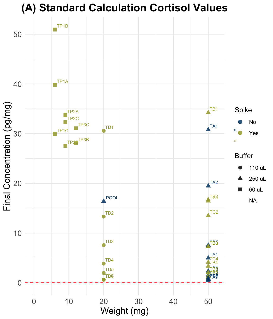
(B) Accounting for Spike
dSpike$Spike <- replace(dSpike$Spike, dSpike$Spike == 1, 'Yes')
dSpike$Spike <- replace(dSpike$Spike, dSpike$Spike == 0, 'No')
dSpike$Buffer <- dSpike$Buffer_ml
dSpike$Buffer <- replace(dSpike$Buffer, dSpike$Buffer == 0.06, '60 uL')
dSpike$Buffer <- replace(dSpike$Buffer, dSpike$Buffer == 0.11, '110 uL')
dSpike$Buffer <- replace(dSpike$Buffer, dSpike$Buffer == 0.25, '250 uL')

# scatterplot
ggplot(dSpike, aes(y = Final_conc_pg.mg,
                 x = Weight_mg,
                 color = Spike,
                 shape = Buffer)) +
  geom_point(size = 3.5,  alpha = 0.85) +
  geom_text(aes(label = Sample), size = 3, vjust = -1, hjust = -0.1) +
  theme_minimal() +
  xlim(0,52) +
  geom_hline(yintercept = 0,
             linetype = "dashed", color = "red") +
  labs(
    title = "(B) Calculation Accounting for Spike",
    y = "Final Concentration (pg/mg)",
    x = "Weight (mg)" ) +
  theme(
    plot.title = element_text(hjust = 0.5,
                              size = 17, face = "bold"),
    axis.title = element_text(size = 14),
    axis.text = element_text(size = 12)
  )+
  scale_color_paletteer_d("vangogh::CafeTerrace")
Warning: Removed 3 rows containing missing values or values outside the scale range
(`geom_point()`).Warning: Removed 3 rows containing missing values or values outside the scale range
(`geom_text()`).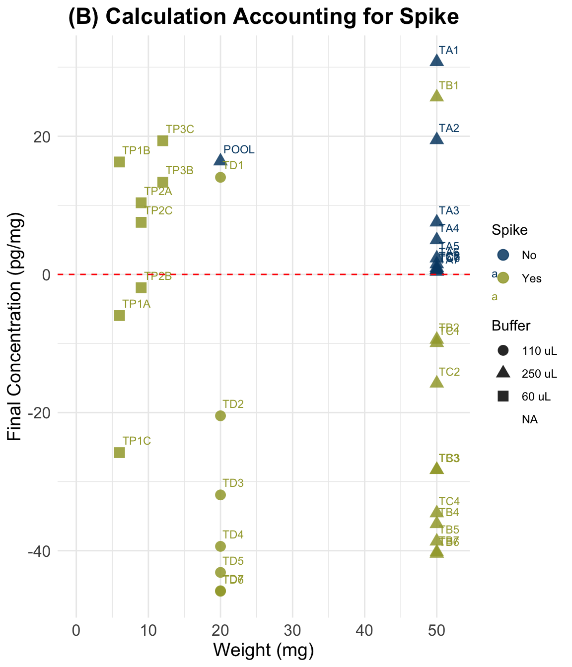
(C)
# scatterplot method c
datac$Spike <- replace(datac$Spike, data$Spike == 1, 'Yes')
datac$Spike <- replace(datac$Spike, data$Spike == 0, 'No')
datac$Buffer <- data$Buffer_ml
datac$Buffer <- replace(datac$Buffer, data$Buffer == 0.06, '60 uL')
datac$Buffer <- replace(datac$Buffer, data$Buffer == 0.11, '110 uL')
datac$Buffer <- replace(datac$Buffer, data$Buffer == 0.25, '250 uL')


ggplot(datac, aes(y = Final_conc_pg.mg,
                 x = Weight_mg,
                 color = Spike,
                 shape = Buffer)) +
  geom_point(size = 2.5, alpha = 0.85) +
   geom_text(aes(label = Sample), size = 2.5, vjust = -0.65, hjust = -0.18) +
    theme_minimal() +
  geom_hline(yintercept = 0,
             linetype = "dashed", color = "red") +
    #ylim(-26,24) +
#  xlim(0,52) +
  labs(
    title = "(C) ",
    y = "Final Concentration (pg/mg)",
    x = "Weight (mg)") +
  theme(
    plot.title = element_text(hjust = 0.5,
                              size = 17, face = "bold"),
    axis.title = element_text(size = 14),
    axis.text = element_text(size = 12)
  ) +
  scale_color_paletteer_d("vangogh::CafeTerrace")
Warning: Removed 3 rows containing missing values or values outside the scale range
(`geom_point()`).Warning: Removed 3 rows containing missing values or values outside the scale range
(`geom_text()`).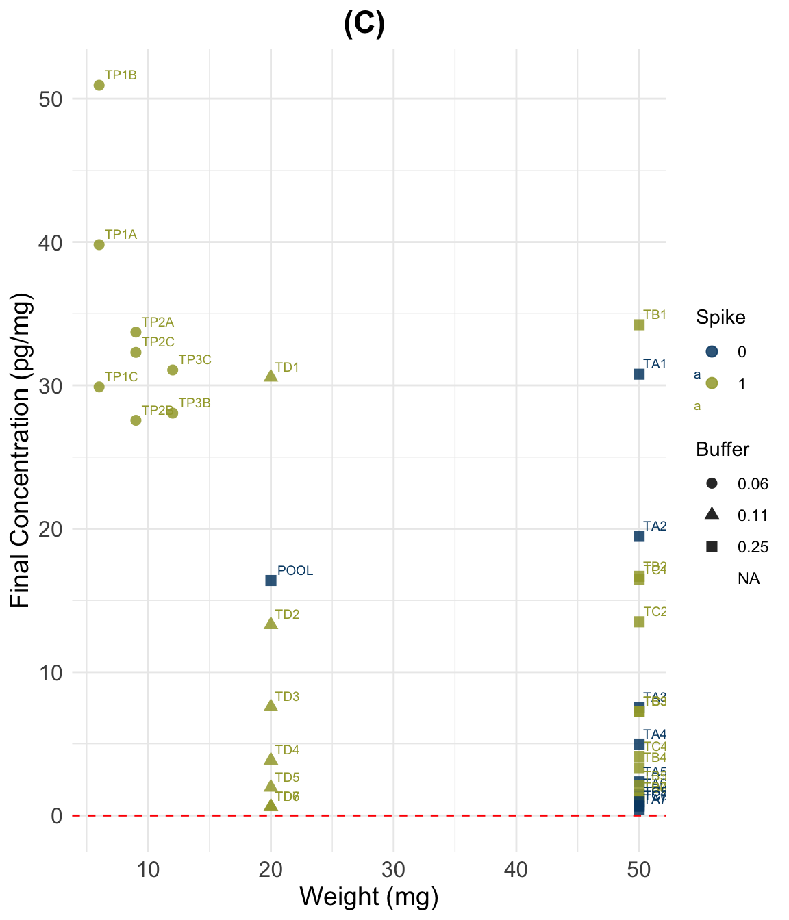
D
dSpiked$Spike <- replace(dSpiked$Spike, dSpiked$Spike == 1, 'Yes')
dSpiked$Spike <- replace(dSpiked$Spike, dSpiked$Spike == 0, 'No')
dSpiked$Buffer <- dSpiked$Buffer_ml
dSpiked$Buffer <- replace(dSpiked$Buffer, dSpiked$Buffer == 0.06, '60 uL')
dSpiked$Buffer <- replace(dSpiked$Buffer, dSpiked$Buffer == 0.11, '110 uL')
dSpiked$Buffer <- replace(dSpiked$Buffer, dSpiked$Buffer == 0.25, '250 uL')

# scatterplot
ggplot(dSpiked, aes(y = Final_conc_pg.mg,
                 x = Weight_mg,
                 color = Spike,
                 shape = Buffer)) +
  geom_point(size = 3.5,  alpha = 0.85) +
  geom_text(aes(label = Sample), size = 3, vjust = -1, hjust = -0.1) +
  theme_minimal() +
    ylim(-26,30) +
  xlim(0,52) +
  geom_hline(yintercept = 0,
             linetype = "dashed", color = "red") +
  labs(
    title = "(D) ",
    y = "Final Concentration (pg/mg)",
    x = "Weight (mg)" ) +
  theme(
    plot.title = element_text(hjust = 0.5,
                              size = 17, face = "bold"),
    axis.title = element_text(size = 14),
    axis.text = element_text(size = 12)
  )+
  scale_color_paletteer_d("vangogh::CafeTerrace")
Warning: Removed 4 rows containing missing values or values outside the scale range
(`geom_point()`).Warning: Removed 4 rows containing missing values or values outside the scale range
(`geom_text()`).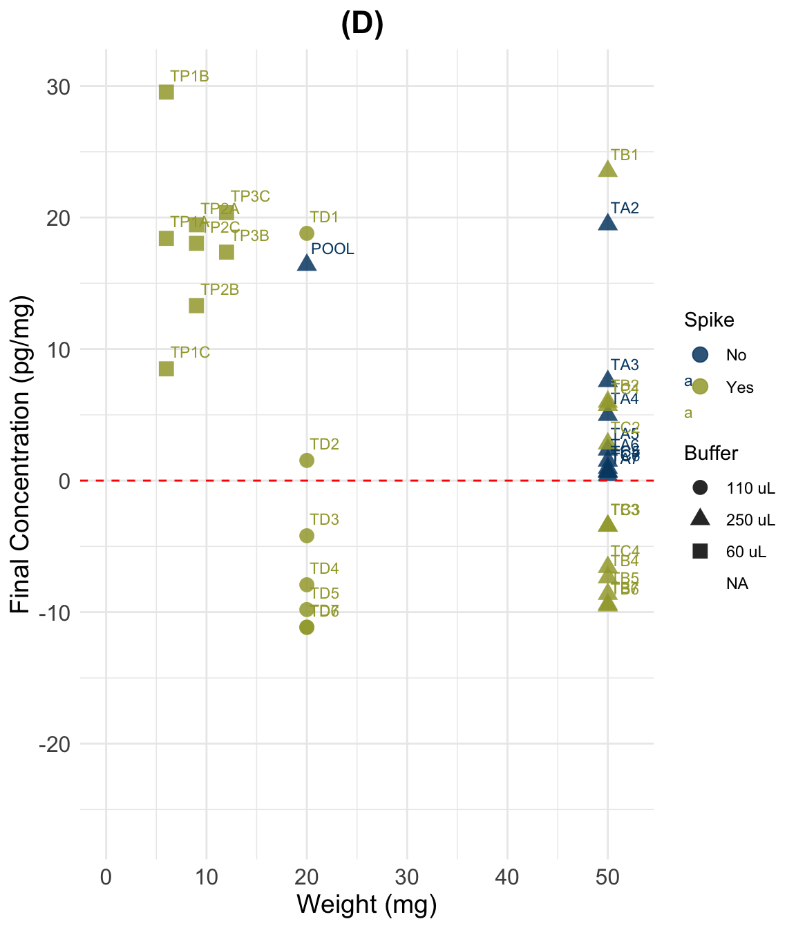
Evaluation
# non-spiked samples only
data2 <-data

#two datasets, separated by dilution
data2.06 <- data2[data2$Buffer == "60 uL", ]
data2.11 <- data2[data2$Buffer == "110 uL", ]
data2.25 <- data2[data2$Buffer == "250 uL", ]


#### fit models ####

# model Buffer = 0.06
model06 <- lm(Final_conc_pg.mg ~ Weight_mg,
              data = data2.06)
r_squared06 <- summary(model06)$r.squared

# model Buffer = 0.25
model25 <- lm(Final_conc_pg.mg ~ Weight_mg,
              data = data2.25)
r_squared25 <- summary(model25)$r.squared

# Calculate residuals
residuals06 <- residuals(model06)
residuals25 <- residuals(model25)

# Quantify residuals
# Mean Absolute Error
mae06 <- mean(abs(residuals06))
# Standard Deviation of Residuals
std_dev06 <- sd(residuals06)

# Mean Absolute Error
mae25 <- mean(abs(residuals25))
# Standard Deviation of Residuals
std_dev25 <- sd(residuals25)


# scatterplot

ggplot(data2, aes(y = Final_conc_pg.mg,
                  x = Weight_mg,
                  color = Category,
                  fill = Category)) +
  geom_point(size = 2.5) +
  geom_text(label = c(data2$Sample), nudge_y = 0.75, nudge_x = -0.5) +
  geom_smooth(method = "lm",
              color = "gold3",
              se = TRUE,
              alpha = 0.1) +
  geom_hline(yintercept = mean(data2$Final_conc_pg.mg),
             color = "gray80",
             linetype = "dashed") +
  geom_hline(yintercept = mean(data2.06$Final_conc_pg.mg),
             color = "lightblue3",
             linetype = "dashed") +
  geom_hline(yintercept = mean(data2.25$Final_conc_pg.mg),
             color = "lightpink3",
             linetype = "dashed") +
  theme_minimal() +
  xlim(5, max(data2$Weight_mg) + 4) +
  ylim(0, max(data2$Final_conc_pg.mg)+4) +
  labs(
    title = "Final Cort Concentration and Weight
    (Non-spiked only)",
    y = "Final Concentration (pg/mg)",
    x = "Weight (mg)"
  ) +
  theme(
    plot.title = element_text(hjust = 0.5, size = 16, face = "bold"),
    axis.title = element_text(size = 14),
    axis.text = element_text(size = 12)
  ) +
  # Add R^2 annotation
  annotate("text", x = max(data2$Weight_mg) * 0.7,
           y = min(data2$Final_conc_pg.mg) * 1.5,
           label = paste("R² =", round(r_squared06, 3)),
           size = 5, color = "black") +
  annotate("text", x = max(data2$Weight_mg) * 0.7,
           y = max(data2$Final_conc_pg.mg) * 0.84,
           label = paste("R² =", round(r_squared25, 3)),
           size = 5, color = "black")
Warning: Removed 3 rows containing non-finite outside the scale range
(`stat_smooth()`).Warning: Removed 3 rows containing missing values or values outside the scale range
(`geom_point()`).Warning: Removed 3 rows containing missing values or values outside the scale range
(`geom_text()`).Warning: Removed 1 row containing missing values or values outside the scale range
(`geom_hline()`).
Removed 1 row containing missing values or values outside the scale range
(`geom_hline()`).
Removed 1 row containing missing values or values outside the scale range
(`geom_hline()`).Warning: Removed 1 row containing missing values or values outside the scale range
(`geom_text()`).
Removed 1 row containing missing values or values outside the scale range
(`geom_text()`).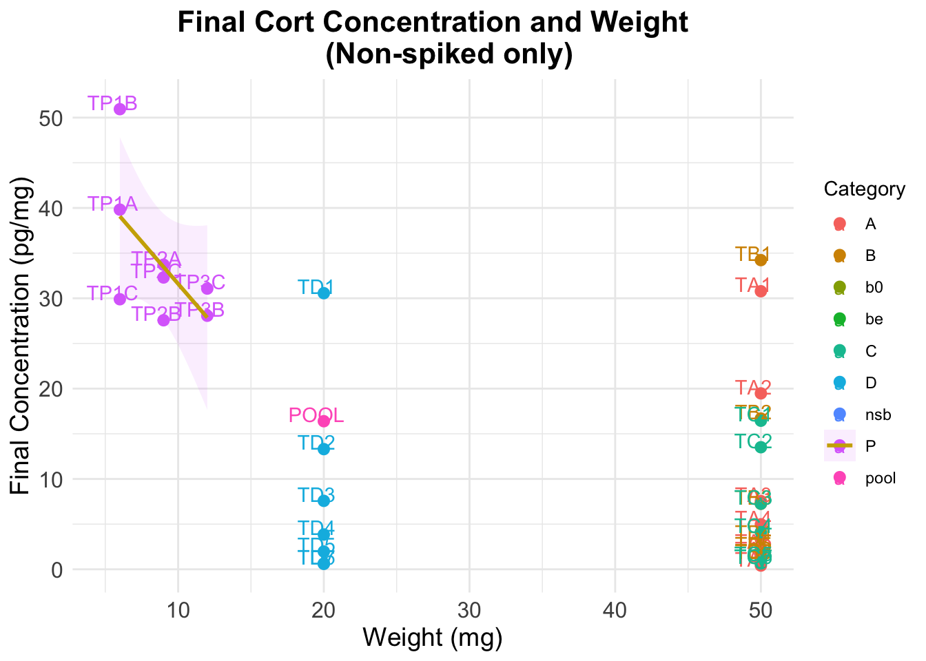
The previous figure shows that:
- results are very stable across weights, particularly for the samples where a dilution of 250 uL was used
- there is more error when using a dilution of 60 uL
- dilution affects estimation of cortisol concentration in a significant way: even though final concentration numbers account for differences in the dilutions, the results we observe for each group do not overlap
- the average value when using 250 uL of buffer is twice as big as when using 60 uL
Optimal dilution
Error using 0.06 mL buffer
Mean Absolute Error (MAE) 0.06 mL: 4.064 Standard Deviation of Residuals 0.06 mL: 6.235 Error using 0.25 mL buffer
Mean Absolute Error (MAE) 0.25 mL: 7.328 Standard Deviation of Residuals 0.25 mL: 9.695 From this we conclude that using a 250 uL dilution provides more consistent results
sessionInfo()R version 4.4.3 (2025-02-28)
Platform: aarch64-apple-darwin20
Running under: macOS Sequoia 15.3.2
Matrix products: default
BLAS: /Library/Frameworks/R.framework/Versions/4.4-arm64/Resources/lib/libRblas.0.dylib
LAPACK: /Library/Frameworks/R.framework/Versions/4.4-arm64/Resources/lib/libRlapack.dylib; LAPACK version 3.12.0
locale:
[1] en_US.UTF-8/en_US.UTF-8/en_US.UTF-8/C/en_US.UTF-8/en_US.UTF-8
time zone: America/Detroit
tzcode source: internal
attached base packages:
[1] stats graphics grDevices utils datasets methods base
other attached packages:
[1] dplyr_1.1.4 paletteer_1.6.0 broom_1.0.7 ggplot2_3.5.1
[5] knitr_1.49
loaded via a namespace (and not attached):
[1] sass_0.4.9 utf8_1.2.4 generics_0.1.3 tidyr_1.3.1
[5] prismatic_1.1.2 lattice_0.22-6 stringi_1.8.4 digest_0.6.37
[9] magrittr_2.0.3 evaluate_1.0.1 grid_4.4.3 fastmap_1.2.0
[13] Matrix_1.7-2 rprojroot_2.0.4 workflowr_1.7.1 jsonlite_1.8.9
[17] backports_1.5.0 rematch2_2.1.2 promises_1.3.0 mgcv_1.9-1
[21] purrr_1.0.2 fansi_1.0.6 scales_1.3.0 jquerylib_0.1.4
[25] cli_3.6.3 rlang_1.1.4 splines_4.4.3 munsell_0.5.1
[29] withr_3.0.2 cachem_1.1.0 yaml_2.3.10 tools_4.4.3
[33] colorspace_2.1-1 httpuv_1.6.15 vctrs_0.6.5 R6_2.5.1
[37] lifecycle_1.0.4 git2r_0.35.0 stringr_1.5.1 fs_1.6.5
[41] pkgconfig_2.0.3 pillar_1.9.0 bslib_0.8.0 later_1.3.2
[45] gtable_0.3.6 glue_1.8.0 Rcpp_1.0.13-1 xfun_0.49
[49] tibble_3.2.1 tidyselect_1.2.1 rstudioapi_0.17.1 farver_2.1.2
[53] nlme_3.1-167 htmltools_0.5.8.1 rmarkdown_2.29 labeling_0.4.3
[57] compiler_4.4.3