Last updated: 2024-11-11

Checks: 7 0

Knit directory: HairCort-Evaluation-Nist2020/

This reproducible R Markdown analysis was created with workflowr (version 1.7.0). The Checks tab describes the reproducibility checks that were applied when the results were created. The Past versions tab lists the development history.

R Markdown file: up-to-date

Great! Since the R Markdown file has been committed to the Git repository, you know the exact version of the code that produced these results.

Environment: empty

Great job! The global environment was empty. Objects defined in the global environment can affect the analysis in your R Markdown file in unknown ways. For reproduciblity it’s best to always run the code in an empty environment.

Seed: set.seed(20241016)

The command set.seed(20241016) was run prior to running the code in the R Markdown file. Setting a seed ensures that any results that rely on randomness, e.g. subsampling or permutations, are reproducible.

Session information: recorded

Great job! Recording the operating system, R version, and package versions is critical for reproducibility.

Cache: none

Nice! There were no cached chunks for this analysis, so you can be confident that you successfully produced the results during this run.

File paths: relative

Great job! Using relative paths to the files within your workflowr project makes it easier to run your code on other machines.

Repository version: 436d20b

Great! You are using Git for version control. Tracking code development and connecting the code version to the results is critical for reproducibility.

The results in this page were generated with repository version 436d20b. See the Past versions tab to see a history of the changes made to the R Markdown and HTML files.

Note that you need to be careful to ensure that all relevant files for the analysis have been committed to Git prior to generating the results (you can use wflow_publish or wflow_git_commit). workflowr only checks the R Markdown file, but you know if there are other scripts or data files that it depends on. Below is the status of the Git repository when the results were generated:


Ignored files:
    Ignored:    .DS_Store
    Ignored:    .Rhistory

Note that any generated files, e.g. HTML, png, CSS, etc., are not included in this status report because it is ok for generated content to have uncommitted changes.

These are the previous versions of the repository in which changes were made to the R Markdown (analysis/Results.Rmd) and HTML (docs/Results.html) files. If you’ve configured a remote Git repository (see ?wflow_git_remote), click on the hyperlinks in the table below to view the files as they were in that past version.

File	Version	Author	Date	Message
Rmd	8c54674	Paloma	2024-11-11	upodaptes
html	8c54674	Paloma	2024-11-11	upodaptes
Rmd	dbfcd66	Paloma	2024-11-11	wflow_rename("./analysis/ELISA_visualizations.Rmd", to = "./analysis/Results.Rmd")
html	dbfcd66	Paloma	2024-11-11	wflow_rename("./analysis/ELISA_visualizations.Rmd", to = "./analysis/Results.Rmd")

Introduction

Here I use QCed results from an ELISA plate. All hair samples were obtained from the same person. I tested 3 variables:

dilution (60 nL vs 250 nL, coded as 0 and 1, respectively)
weight (11 to 37.1 mg)
spike (25 nL stock solution (1:10) added to some wells, coded as 0 and 1, meaning not-spiked and spiked)

I removed the samples that have a Coef of variation higher than 15%.

Summary of results

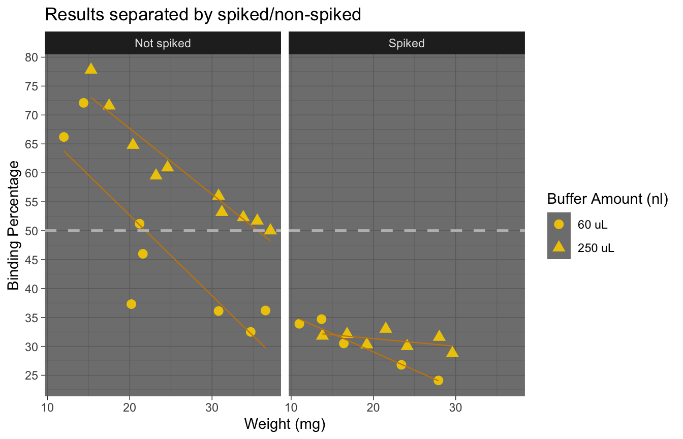
The figures below were used to decide that the optimal parameters are:

Weight higher than 20, ideally. Binding deviation goes down with higher weight.
Dilution between 60 and 250 ul (higher dilution provides lower coef. of variation, more lower dilutions locate samples closer to 50% binding. An intermedieate value would be best)
Spike Non-spiked samples provide lower binding deviation from 50% (i.e. measures are close to falling outside the curve)

Version	Author	Date
dbfcd66	Paloma	2024-11-11

Here we see the effect of the spike more clearly: adding a spike may not be necessary unless we have very small samples.

Spiked samples were removed due to inconsistent results.

Version	Author	Date
dbfcd66	Paloma	2024-11-11

Results

Version	Author	Date
dbfcd66	Paloma	2024-11-11

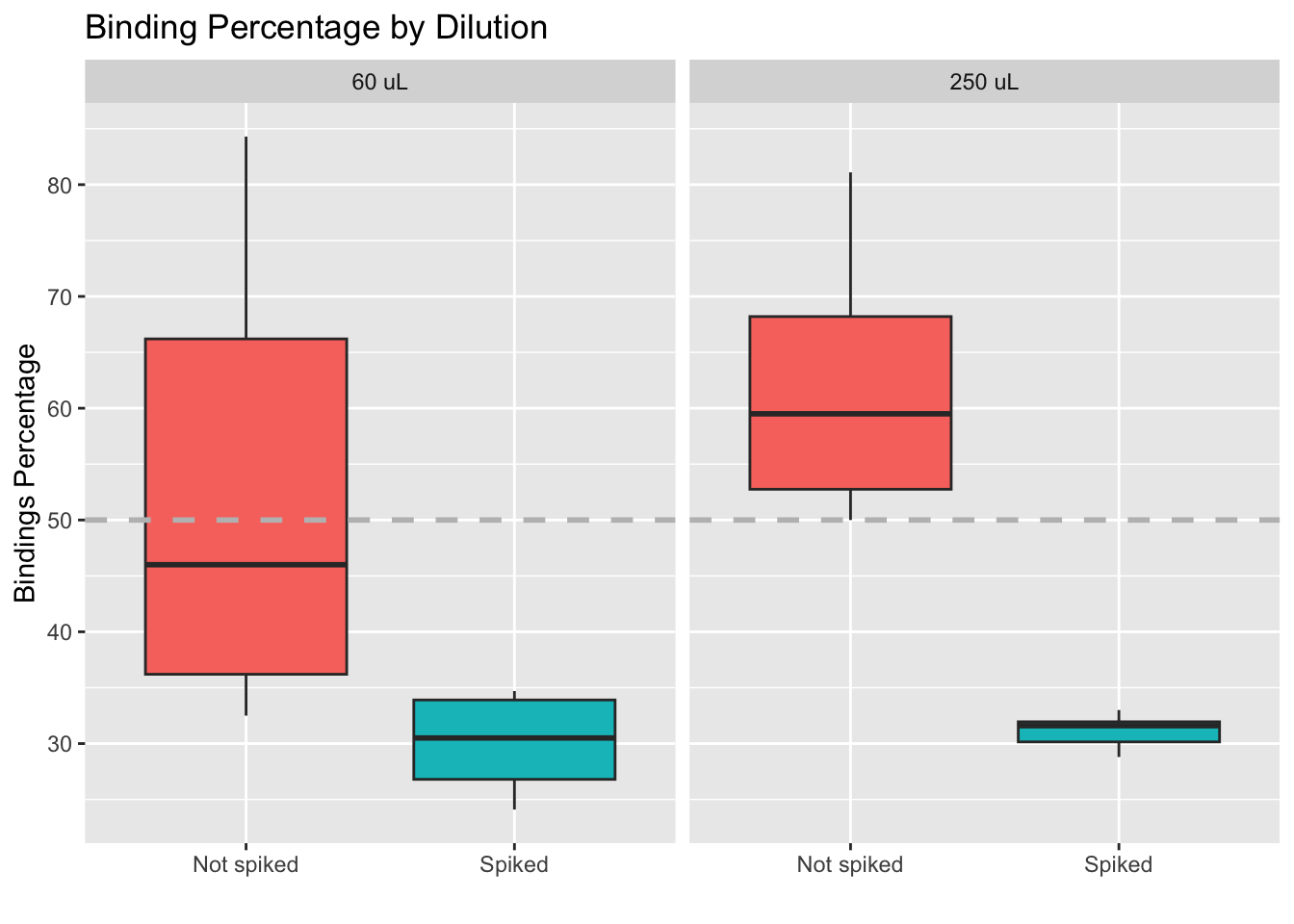
The following plots were made considering that having a binding of 50% is ideal. Data points that are over 80% or under 20% are not within the curve, and predictions are less accurate.

Binding percentages

Binding percentage by different variables

Version	Author	Date
dbfcd66	Paloma	2024-11-11

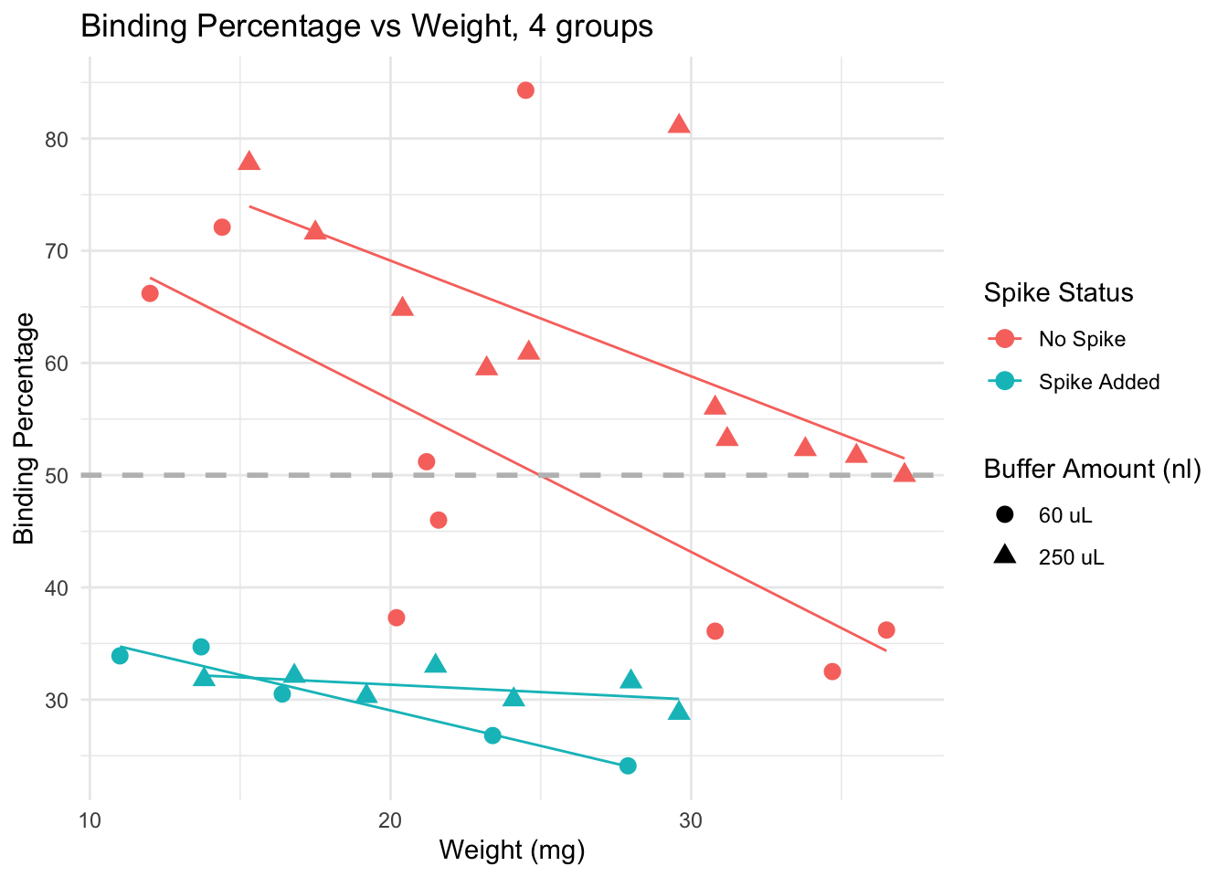
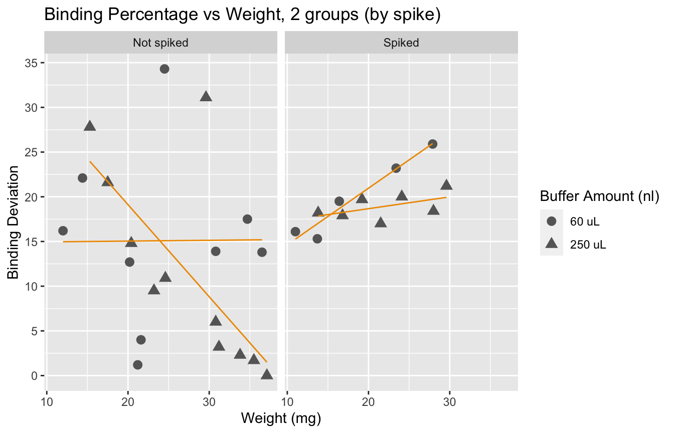
Spiked samples (turquoise) have lower binding, because they have higher levels of cortisol than non spiked (pink) samples.
Dilution: effect is less clear. We see samples with both 60 uL and 250 uL binding at very high and very low levels.
Trends: within non-spiked samples with a similar weight and diluted at 60uL (pink circles), we do not obtain consistent binding percentages. However, non-spiked samples with similar weights do obtain similar bindings, and the lines are in the expected direction (higher weight, lower binding), except by a few outliers that would be removed from the analysis anyway (for having binding over 80%)
Conclusion: samples across different weights, non-spiked, and diluted in 250 uL buffer seem to provide the best results, particularly if samples weigh more than 15 mg. Using less than that may be risky, and in those cases, it may be better to use less buffer to concentrate the samples a bit more.

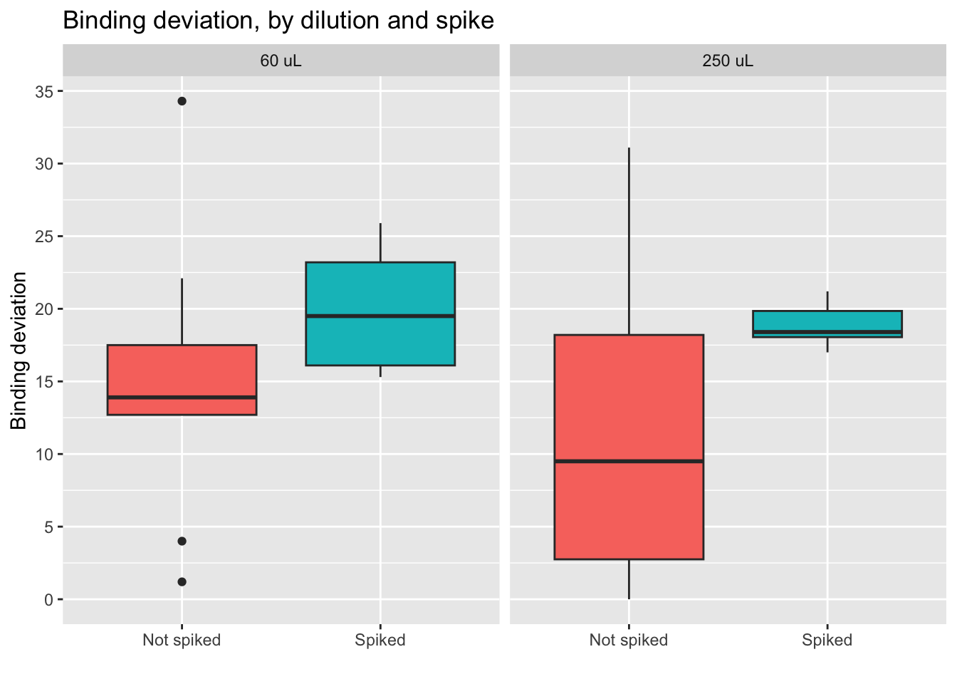
Value distributions by group (boxplots)

Version	Author	Date
dbfcd66	Paloma	2024-11-11

Here we also see that the impact of the spike on the values is larger than the impact of using a different dilution

Coef. of variation percentage

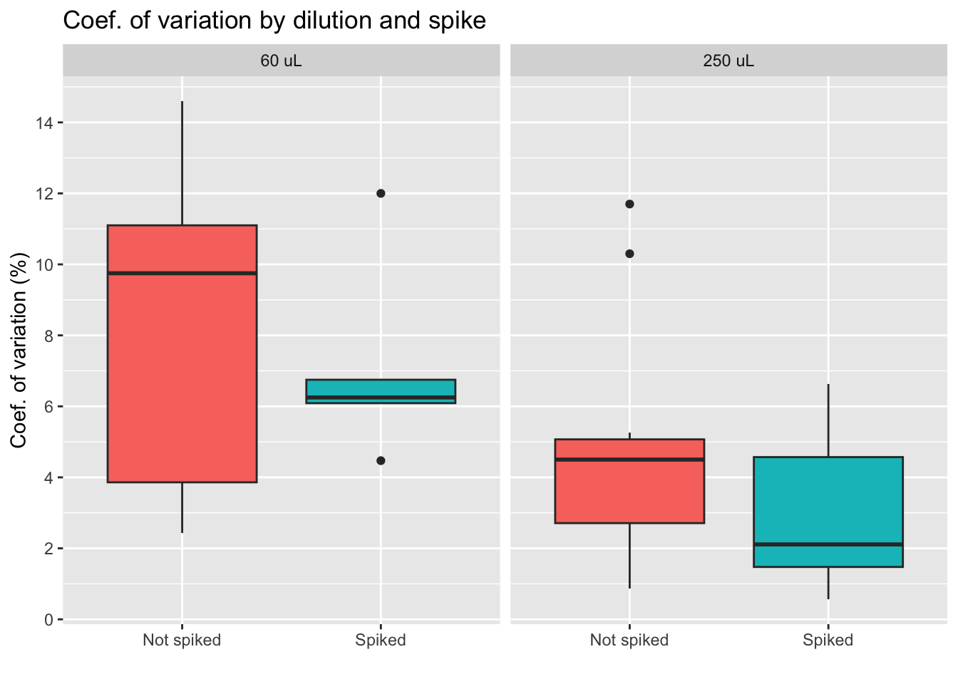
The coefficient of variation or CV is a standardized measure of the difference between duplicates (same sample, same weight, same dilution, same everything). Some variables may make duplicates more variable, so this is what will be tested below.

Coef. of variation by group

Version	Author	Date
dbfcd66	Paloma	2024-11-11

Conclusion diluting the sample less seems to lead to higher differences between duplicates, which is something we want to avoid. We also see less variation for the group of spiked samples, with the lowest average of the four groups. Yet, we also must note that the spiked, 250 uL group has only 6 samples, as we see on the table below.

Dilution:	No spike	Spiked
60 uL	7	7
250 uL	12	6
Total: 32 samples

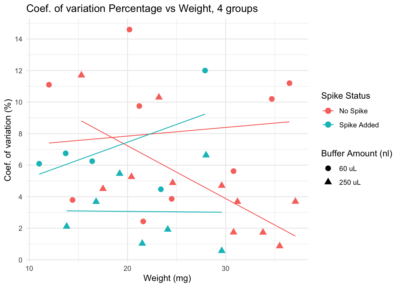
Coef. of variation by different variables

Version	Author	Date
4c08739	Paloma	2024-11-11

Lower CV is seen in spiked + 250 uL group, particularly for samples with low weight. Yet, non spiked, diluted in 250uL samples have very low CV if weight is over 30.

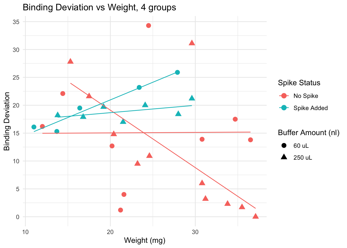
Deviation from 50% binding

Here I calculate a “binding” deviation score, to have a better idea of the “distance” between the values obtained and what I should aim for: 50% binding. Here an example of how this score works:

	Sample	Binding.Perc	Binding_deviation
22	32	50.0	0.0
21	31	51.2	1.2
24	34	51.7	1.7
23	33	52.3	2.3
25	36	53.2	3.2
15	27	46.0	4.0

Version	Author	Date
dbfcd66	Paloma	2024-11-11

This plot suggests that for samples of weight lower than 20 mg, adding a spike lowers the binding deviation. This effect is lost if samples are heaver than 20 mg.

Version	Author	Date
dbfcd66	Paloma	2024-11-11

We observe that spiked samples have a higher deviation from the ideal binding. We also observe that having larger samples leads to values closer to 50%. It is interesting to see that error does not go below 15% if we look at samples with weight under 20mg. Yet, we know that a deviation of up to 30% is acceptable.

Version	Author	Date
dbfcd66	Paloma	2024-11-11

Here we see how the lowest (best) scores are obtained by the non-spiked groups. Even better results are obtained if the dilution is 250 uL.

Conclusion: using a 250 uL dilution, without spikes, will lead to better results that fall in the middle of the curve, and allow for more precise calculations of cortisol concentration.

Analysis: linear models

To explore the effects of each variable more systematically, I run multiple models and compared them using AIC Akakikes’ coefficient. I removed samples with a binding over 80% or under 20%.

Version	Author	Date
dbfcd66	Paloma	2024-11-11

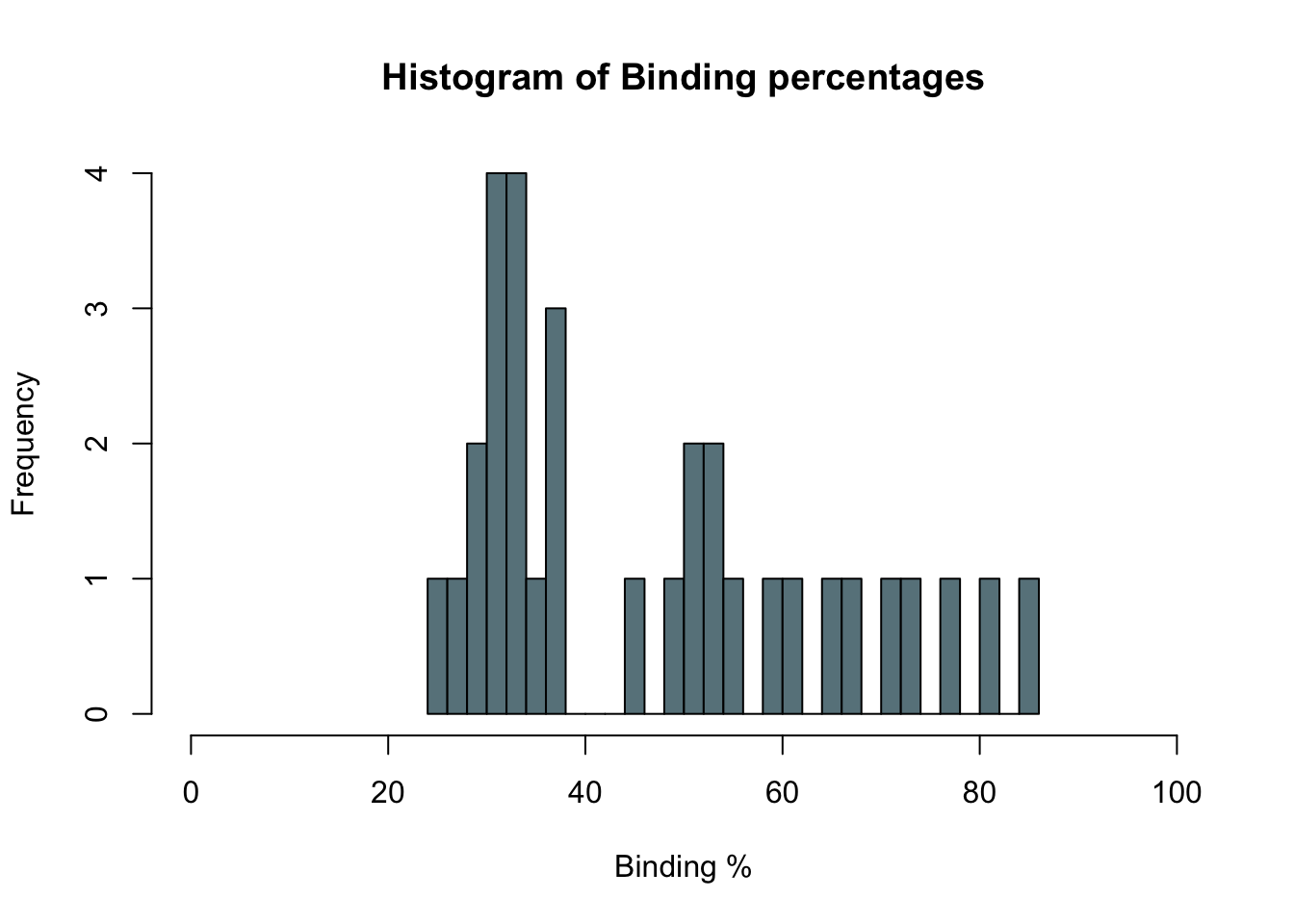
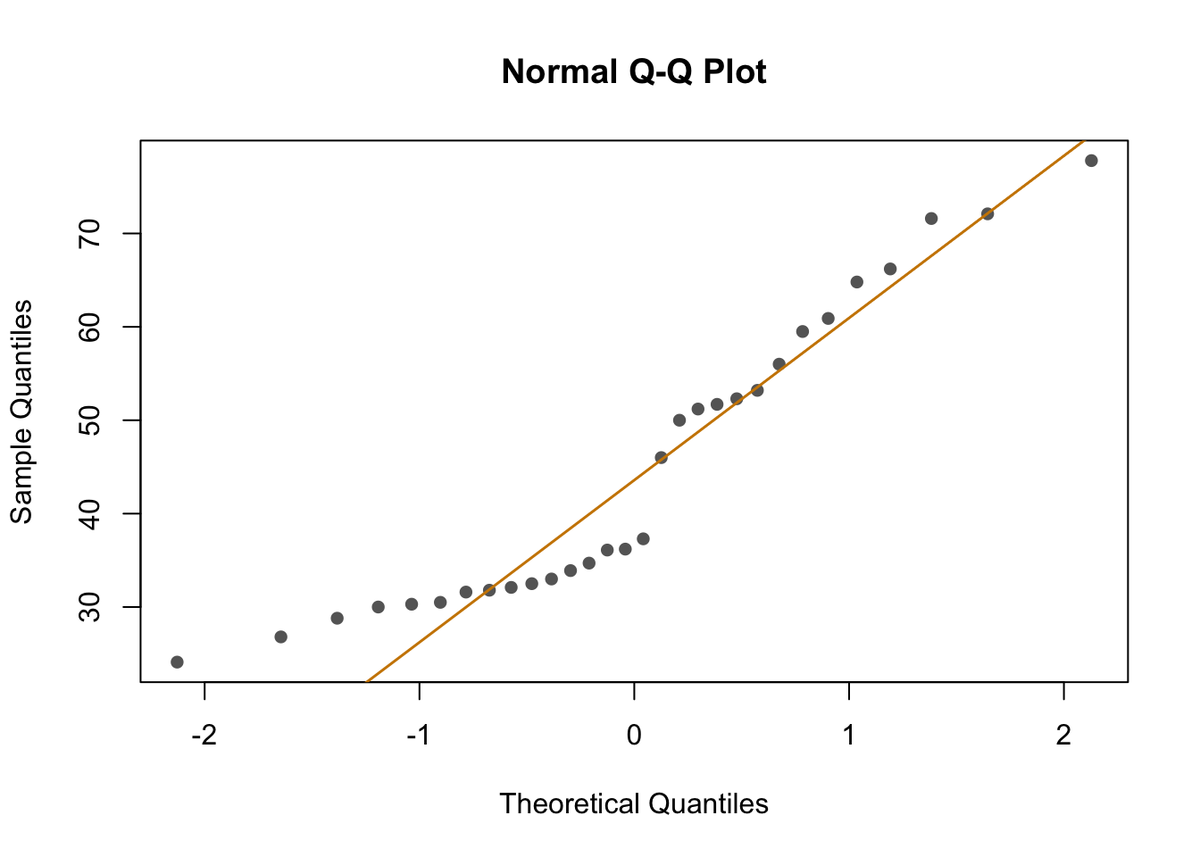
First, I looked at the distribution of the data (binding percentage). I am not sure how to describe it, but it does not look very linear. I will test different distributions at another time, but for now, I will run and compare simple models that should allow me to understand which variables have a greater impact on binding percentages.

Comparing models

# creating function to extract coeffs
extract_coefs <- function(model, model_name) {
  # Extract summary of the model
  coef_summary <- summary(model)$coefficients
  
  # Create a data frame with term names, estimates, and standard errors
  coef_df <- data.frame(
    term = rownames(coef_summary),
    estimate = coef_summary[, "Estimate"],
    std.error = coef_summary[, "Std. Error"],
    model = model_name  # Add the model name as a new column
  )
  
  # Return the data frame
  return(coef_df)
}

binding <- data$Binding.Perc
weight <- data$Weight_mg
spike <- data$Spike
buffer <- data$Buffer_nl

# model 1

m1 <- lm(binding ~ weight)
summary(m1)


Call:
lm(formula = binding ~ weight)

Residuals:
   Min     1Q Median     3Q    Max 
-19.39 -14.46  -5.65  12.69  30.62 

Coefficients:
            Estimate Std. Error t value Pr(>|t|)    
(Intercept)  51.6739     9.2460   5.589 5.56e-06 ***
weight       -0.2934     0.3732  -0.786    0.438    
---
Signif. codes:  0 '***' 0.001 '**' 0.01 '*' 0.05 '.' 0.1 ' ' 1

Residual standard error: 15.77 on 28 degrees of freedom
Multiple R-squared:  0.0216,    Adjusted R-squared:  -0.01335 
F-statistic: 0.618 on 1 and 28 DF,  p-value: 0.4384

confint(m1, level = 0.95)

                2.5 %     97.5 %
(Intercept) 32.734311 70.6134504
weight      -1.057979  0.4711297

# model 2

m2 <- lm(binding ~ spike)
summary(m2)


Call:
lm(formula = binding ~ spike)

Residuals:
     Min       1Q   Median       3Q      Max 
-21.6889  -3.6222  -0.2333   3.8667  23.6111 

Coefficients:
            Estimate Std. Error t value Pr(>|t|)    
(Intercept)   54.189      2.490  21.765  < 2e-16 ***
spike1       -23.556      3.937  -5.984 1.91e-06 ***
---
Signif. codes:  0 '***' 0.001 '**' 0.01 '*' 0.05 '.' 0.1 ' ' 1

Residual standard error: 10.56 on 28 degrees of freedom
Multiple R-squared:  0.5612,    Adjusted R-squared:  0.5455 
F-statistic: 35.81 on 1 and 28 DF,  p-value: 1.912e-06

confint(m2, level = 0.95)

                2.5 %    97.5 %
(Intercept)  49.08898  59.28880
spike1      -31.61922 -15.49189

# model 3

m3 <- lm(binding ~ buffer)
summary(m3)


Call:
lm(formula = binding ~ buffer)

Residuals:
    Min      1Q  Median      3Q     Max 
-19.165 -14.670  -3.835   9.970  31.515 

Coefficients:
            Estimate Std. Error t value Pr(>|t|)    
(Intercept)   40.585      4.296   9.447 3.33e-10 ***
buffer1        7.380      5.707   1.293    0.207    
---
Signif. codes:  0 '***' 0.001 '**' 0.01 '*' 0.05 '.' 0.1 ' ' 1

Residual standard error: 15.49 on 28 degrees of freedom
Multiple R-squared:  0.05636,   Adjusted R-squared:  0.02266 
F-statistic: 1.672 on 1 and 28 DF,  p-value: 0.2065

confint(m3, level = 0.95)

                2.5 %   97.5 %
(Intercept) 31.784638 49.38459
buffer1     -4.309996 19.07018

# model 4

m4 <- lm(binding ~ weight + spike)
summary(m4)


Call:
lm(formula = binding ~ weight + spike)

Residuals:
    Min      1Q  Median      3Q     Max 
-21.621  -4.416   1.329   6.013  14.585 

Coefficients:
            Estimate Std. Error t value Pr(>|t|)    
(Intercept)  76.6215     5.7290  13.374 2.00e-13 ***
weight       -0.8763     0.2100  -4.172  0.00028 ***
spike1      -28.0684     3.3078  -8.485 4.25e-09 ***
---
Signif. codes:  0 '***' 0.001 '**' 0.01 '*' 0.05 '.' 0.1 ' ' 1

Residual standard error: 8.388 on 27 degrees of freedom
Multiple R-squared:  0.7332,    Adjusted R-squared:  0.7134 
F-statistic: 37.09 on 2 and 27 DF,  p-value: 1.795e-08

confint(m4, level = 0.95)

                 2.5 %      97.5 %
(Intercept)  64.866499  88.3764142
weight       -1.307243  -0.4453015
spike1      -34.855427 -21.2812872

# model 5 

m5 <- lm(binding ~ weight + buffer)
summary(m5)


Call:
lm(formula = binding ~ weight + buffer)

Residuals:
     Min       1Q   Median       3Q      Max 
-20.5867 -13.8305   0.2964  10.4043  28.5410 

Coefficients:
            Estimate Std. Error t value Pr(>|t|)    
(Intercept)  49.3231     9.1936   5.365 1.14e-05 ***
weight       -0.4003     0.3726  -1.074    0.292    
buffer1       8.5875     5.8012   1.480    0.150    
---
Signif. codes:  0 '***' 0.001 '**' 0.01 '*' 0.05 '.' 0.1 ' ' 1

Residual standard error: 15.45 on 27 degrees of freedom
Multiple R-squared:  0.09504,   Adjusted R-squared:  0.02801 
F-statistic: 1.418 on 2 and 27 DF,  p-value: 0.2597

confint(m5, level = 0.95)

                2.5 %     97.5 %
(Intercept) 30.459445 68.1867374
weight      -1.164810  0.3642451
buffer1     -3.315599 20.4905160

# model 6

m6 <- lm(binding ~ spike + buffer)
summary(m6)


Call:
lm(formula = binding ~ spike + buffer)

Residuals:
    Min      1Q  Median      3Q     Max 
-17.230  -5.022  -1.865   4.197  22.370 

Coefficients:
            Estimate Std. Error t value Pr(>|t|)    
(Intercept)   49.730      3.093  16.077 2.37e-15 ***
spike1       -23.778      3.693  -6.438 6.73e-07 ***
buffer1        8.026      3.651   2.198   0.0367 *  
---
Signif. codes:  0 '***' 0.001 '**' 0.01 '*' 0.05 '.' 0.1 ' ' 1

Residual standard error: 9.907 on 27 degrees of freedom
Multiple R-squared:  0.6278,    Adjusted R-squared:  0.6002 
F-statistic: 22.77 on 2 and 27 DF,  p-value: 1.607e-06

confint(m6, level = 0.95)

                  2.5 %    97.5 %
(Intercept)  43.3835259  56.07685
spike1      -31.3568589 -16.20012
buffer1       0.5335106  15.51781

# model 7

m7 <- lm(binding ~ weight + buffer + spike)
summary(m7)


Call:
lm(formula = binding ~ weight + buffer + spike)

Residuals:
     Min       1Q   Median       3Q      Max 
-16.2258  -2.0491   0.4047   3.4737  12.5351 

Coefficients:
            Estimate Std. Error t value Pr(>|t|)    
(Intercept)  74.5586     4.2587  17.507 6.57e-16 ***
weight       -1.0412     0.1591  -6.546 6.11e-07 ***
buffer1      11.3144     2.3411   4.833 5.22e-05 ***
spike1      -29.2322     2.4583 -11.891 5.13e-12 ***
---
Signif. codes:  0 '***' 0.001 '**' 0.01 '*' 0.05 '.' 0.1 ' ' 1

Residual standard error: 6.204 on 26 degrees of freedom
Multiple R-squared:  0.8594,    Adjusted R-squared:  0.8432 
F-statistic: 52.99 on 3 and 26 DF,  p-value: 3.261e-11

confint(m7, level = 0.95)

                 2.5 %      97.5 %
(Intercept)  65.804710  83.3124949
weight       -1.368173  -0.7142862
buffer1       6.502196  16.1265526
spike1      -34.285345 -24.1790066

# model 8

sp1 <- data[data$Spike == 1,]
sp0 <- data[data$Spike == 0,]

binding1 <- sp1$Binding.Perc
weight1 <- sp1$Weight_mg
spike1 <- sp1$Spike
buffer1 <- sp1$Buffer_nl

m8 <- lm(binding1 ~  buffer1 + weight1)
summary(m8)


Call:
lm(formula = binding1 ~ buffer1 + weight1)

Residuals:
   Min     1Q Median     3Q    Max 
-2.343 -1.448 -0.262  1.241  2.886 

Coefficients:
            Estimate Std. Error t value Pr(>|t|)    
(Intercept)  37.0130     2.1167  17.486 2.96e-08 ***
buffer11      2.3673     1.2525   1.890  0.09133 .  
weight1      -0.3795     0.1032  -3.678  0.00509 ** 
---
Signif. codes:  0 '***' 0.001 '**' 0.01 '*' 0.05 '.' 0.1 ' ' 1

Residual standard error: 2.055 on 9 degrees of freedom
Multiple R-squared:  0.6144,    Adjusted R-squared:  0.5287 
F-statistic:  7.17 on 2 and 9 DF,  p-value: 0.01373

# model 9
binding0 <- sp0$Binding.Perc
weight0 <- sp0$Weight_mg
spike0 <- sp0$Spike
buffer0 <- sp0$Buffer_nl

m9 <- lm(binding0 ~  buffer0 + weight0)
summary(m9)


Call:
lm(formula = binding0 ~ buffer0 + weight0)

Residuals:
     Min       1Q   Median       3Q      Max 
-14.6241  -2.2477   0.1961   3.0228  12.8202 

Coefficients:
            Estimate Std. Error t value Pr(>|t|)    
(Intercept)  77.5421     4.6585  16.645 4.43e-11 ***
buffer01     16.4037     2.8246   5.807 3.45e-05 ***
weight0      -1.2682     0.1745  -7.269 2.74e-06 ***
---
Signif. codes:  0 '***' 0.001 '**' 0.01 '*' 0.05 '.' 0.1 ' ' 1

Residual standard error: 5.851 on 15 degrees of freedom
Multiple R-squared:  0.8303,    Adjusted R-squared:  0.8077 
F-statistic: 36.69 on 2 and 15 DF,  p-value: 1.67e-06

coef_df1 <- extract_coefs(m1, "Model 1")
coef_df2 <- extract_coefs(m2, "Model 2")
coef_df3 <- extract_coefs(m3, "Model 3")
coef_df4 <- extract_coefs(m4, "Model 4")
coef_df5 <- extract_coefs(m5, "Model 5")
coef_df6 <- extract_coefs(m6, "Model 6")
coef_df7 <- extract_coefs(m7, "Model 7")
coef_df8 <- extract_coefs(m8, "Model 8")
coef_df9 <- extract_coefs(m9, "Model 9")

# Combine the data frames for plotting
coef_df <- rbind(coef_df1, coef_df2, coef_df3, coef_df4)

Plot regression coefs

Plot model 1 to 4

ggplot(coef_df, aes(x = term, y = estimate, color = model)) +
  geom_point(position = position_dodge(width = 4)) +  # Points for the estimates
  geom_errorbar(aes(ymin = estimate - 1.96 * std.error, ymax = estimate + 1.96 * std.error),
                position = position_dodge(width = 0.85), width = 1) +  # Error bars for confidence intervals
  theme_minimal() +
  coord_flip() +  # Flip the coordinates for better readability
  facet_wrap(~ model, ncol = 1) +  # One model per line
  labs(title = "Coefficient Plot for Models 1-4",
       x = "Terms",
       y = "Estimates") +
  theme(legend.position = "none") +
  geom_hline(yintercept = 0, color = "gray", linetype = "dashed") +  # Gray line at zero
  expand_limits(y = c(-58, 58)) +
  theme(
    axis.text.x = element_text(size = 12),        # X-axis text size
    axis.text.y = element_text(size = 12),        # Y-axis text size
    axis.title.x = element_text(size = 14),       # X-axis title size
    axis.title.y = element_text(size = 14),       # Y-axis title size
    plot.title = element_text(size = 16, hjust = 0.5),  # Plot title size and centering
    strip.text = element_text(size = 14)          # Facet label text size
  )

Warning: `position_dodge()` requires non-overlapping x intervals
`position_dodge()` requires non-overlapping x intervals
`position_dodge()` requires non-overlapping x intervals
`position_dodge()` requires non-overlapping x intervals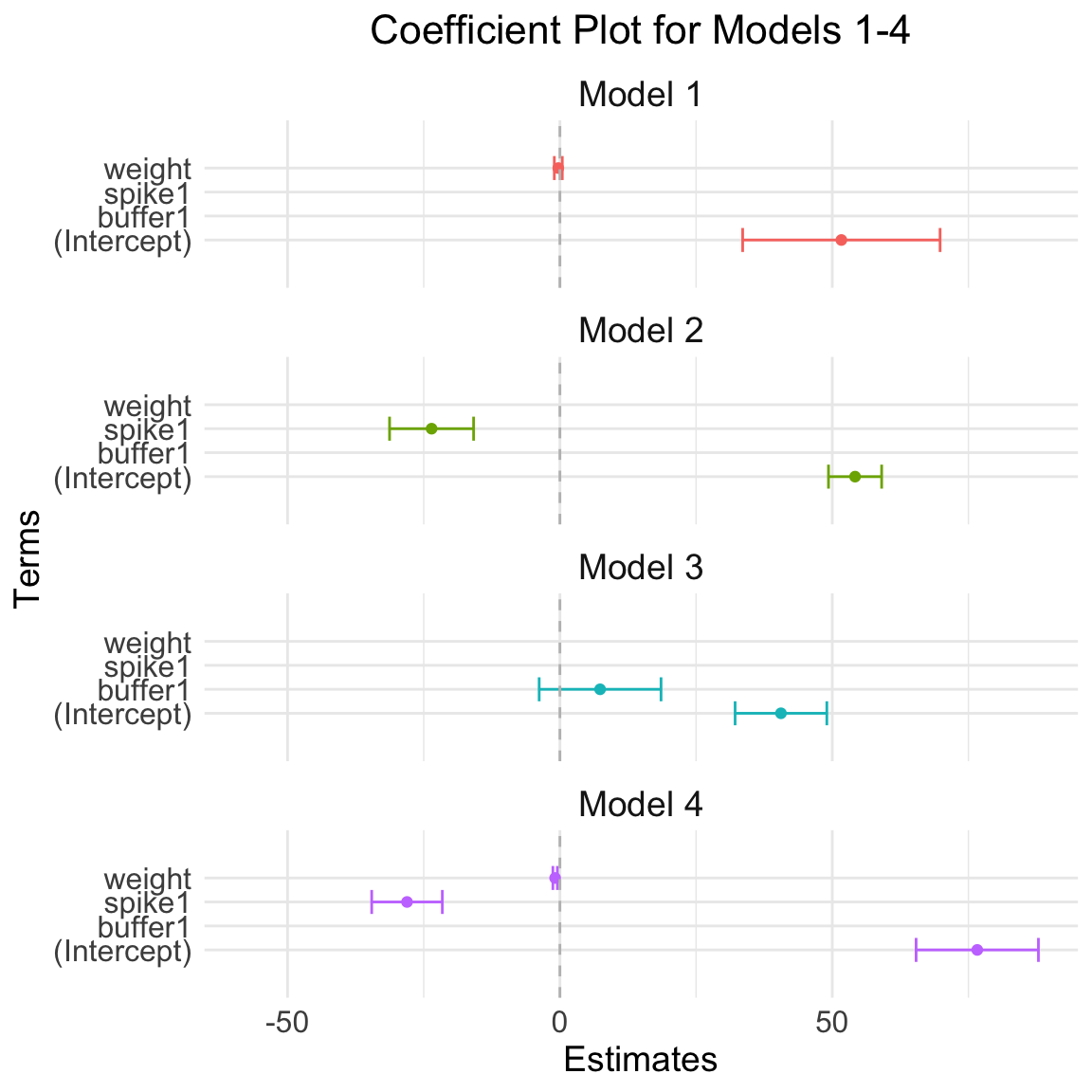

Version	Author	Date
dbfcd66	Paloma	2024-11-11

Plot model 5 to 9

# Combine the data frames for plotting
coef_df <- rbind(coef_df5, coef_df6, coef_df7, coef_df8,coef_df9)

ggplot(coef_df, aes(x = term, y = estimate, color = model)) +
  geom_point(position = position_dodge(width = 3)) +  # Points for the estimates
  geom_errorbar(aes(ymin = estimate - 1.96 * std.error, ymax = estimate + 1.96 * std.error),
                position = position_dodge(width = 0.9), width = 0.85) +  # Error bars for confidence intervals
  theme_minimal() +
  coord_flip() +  # Flip the coordinates for better readability
  facet_wrap(~ model, ncol = 1) +  # One model per line
  labs(title = "Coefficient Plot for Model 5 to 9",
       x = "Terms",
       y = "Estimates") +
  theme(legend.position = "none") +
  geom_hline(yintercept = 0, color = "gray", linetype = "dashed") +  # Gray line at zero
  expand_limits(y = c(-60, 60)) +
  theme(
    axis.text.x = element_text(size = 12),        # X-axis text size
    axis.text.y = element_text(size = 12),        # Y-axis text size
    axis.title.x = element_text(size = 14),       # X-axis title size
    axis.title.y = element_text(size = 14),       # Y-axis title size
    plot.title = element_text(size = 16, hjust = 0.5),  # Plot title size and centering
    strip.text = element_text(size = 14)          # Facet label text size
  )

Warning: `position_dodge()` requires non-overlapping x intervals
`position_dodge()` requires non-overlapping x intervals
`position_dodge()` requires non-overlapping x intervals
`position_dodge()` requires non-overlapping x intervals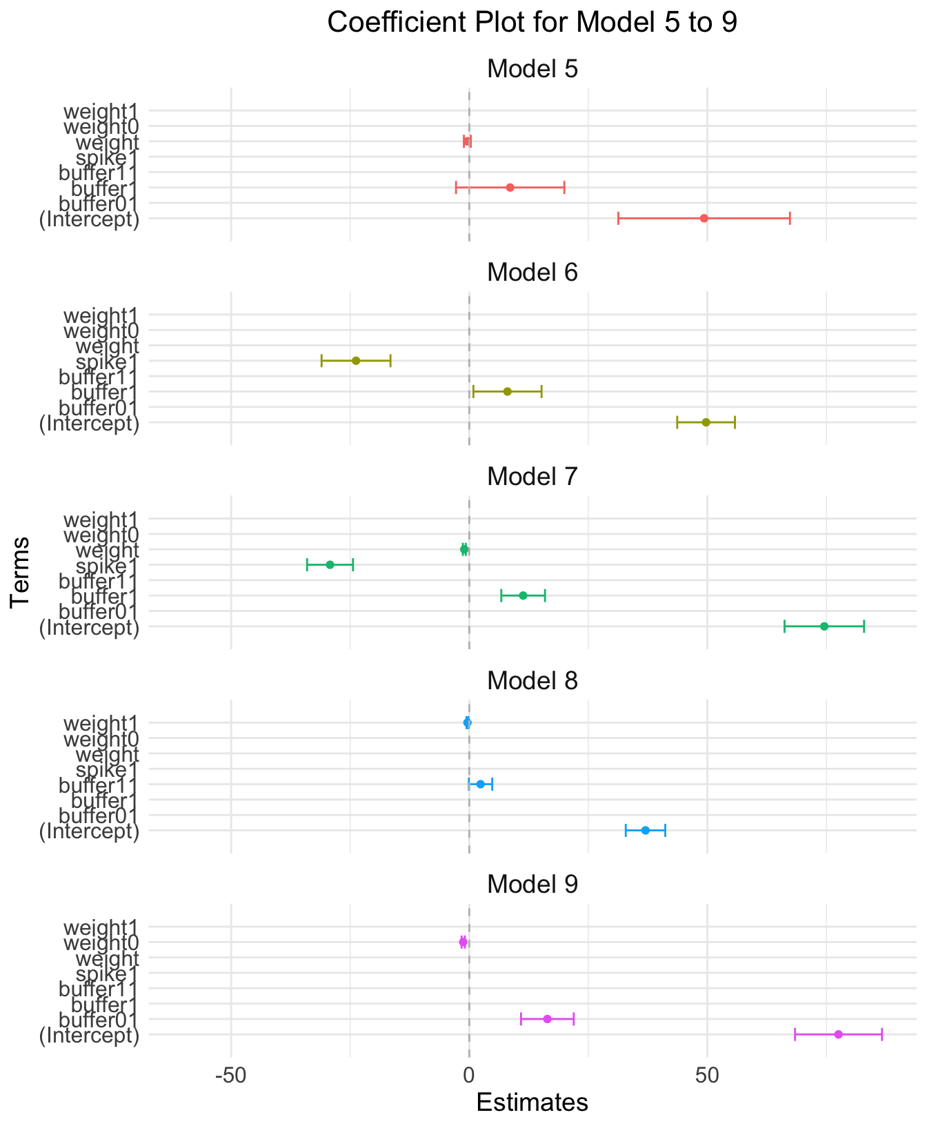

Version	Author	Date
dbfcd66	Paloma	2024-11-11

Summarize info multiple models

model_names <- paste("m", 1:9, sep="")
r_values <- 1:9
all_models <- list(m1, m2, m3, m4, m5, m6, m7, m8, m9)
model_info <- c("weight", "spike", "buffer", "weight + spike", "weight + buffer", "spike + buffer", "spike + buffer + weight", "buffer + weight, spiked only","buffer + weight, NOT spiked only")
sum_models <- as.data.frame(r_values, row.names=model_names)
sum_models$res_std_error <- 1:length(model_names)
sum_models$info <- model_info

for (i in 1:length(model_names)) {
    sum_models$r_values[i]      <- summary(all_models[[i]])$adj.r.squared
    sum_models$res_std_error[i] <- summary(all_models[[i]])$sigma
}

kable(sum_models[order(sum_models$r_values, decreasing = TRUE), ])

	r_values	res_std_error	info
m7	0.8432246	6.203728	spike + buffer + weight
m9	0.8076695	5.850626	buffer + weight, NOT spiked only
m4	0.7134063	8.387781	weight + spike
m6	0.6001972	9.906874	spike + buffer
m2	0.5454965	10.562881	spike
m8	0.5287000	2.054609	buffer + weight, spiked only
m5	0.0280065	15.447046	weight + buffer
m3	0.0226583	15.489485	buffer
m1	-0.0133472	15.772222	weight

Comparing models using Akakike’s information criteria

# computing bias-adjusted version of AIC (AICc) Akakaike's information criteria table
AICc_compare <-AICtab(m1, m2, m3, m4, m5, m6, m7, m8, m9, 
        base = TRUE,
        weights = TRUE,
        logLik  = TRUE,
        #indicate number of observations
        nobs = 30)
kable(AICc_compare)

	logLik	AIC	dLogLik	dAIC	df	weight
m8	-23.94220	55.8844	100.3385734	0.00000	4	1
m9	-55.69788	119.3958	68.5828959	63.51136	4	0
m7	-95.17615	200.3523	29.1046184	144.46791	5	0
m4	-104.79103	217.5821	19.4897423	161.69766	4	0
m6	-109.78461	227.5692	14.4961574	171.68483	4	0
m2	-112.25364	230.5073	12.0271289	174.62289	3	0
m3	-123.73810	253.4762	0.5426679	197.59181	3	0
m5	-123.11028	254.2206	1.1704906	198.33617	4	0
m1	-124.28077	254.5615	0.0000000	198.67715	3	0

# Coef table 
coeftab(m1, m2, m3, m4, m5, m6, m7, m8, m9) -> coeftabs
kable(coeftabs)

	(Intercept)	weight	spike1	buffer1	buffer11	weight1	buffer01	weight0
m1	51.67388	-0.2934245	NA	NA	NA	NA	NA	NA
m2	54.18889	NA	-23.55556	NA	NA	NA	NA	NA
m3	40.58462	NA	NA	7.380090	NA	NA	NA	NA
m4	76.62146	-0.8762722	-28.06836	NA	NA	NA	NA	NA
m5	49.32309	-0.4002825	NA	8.587459	NA	NA	NA	NA
m6	49.73019	NA	-23.77849	8.025660	NA	NA	NA	NA
m7	74.55860	-1.0412296	-29.23218	11.314374	NA	NA	NA	NA
m8	37.01296	NA	NA	NA	2.367304	-0.3794893	NA	NA
m9	77.54213	NA	NA	NA	NA	NA	16.40368	-1.268219

par(mfrow = c(3, 3))

plot(m1, which = 1)  
plot(m2, which = 1, main = "m2")  
plot(m3, which = 1, main = "m3")  
plot(m4, which = 1, main = "m4")
plot(m5, which = 1, main = "m5") 
plot(m6, which = 1, main = "m6")
plot(m7, which = 1, main = "m7")
plot(m8, which = 1, main = "m8")
plot(m9, which = 1, main = "m9")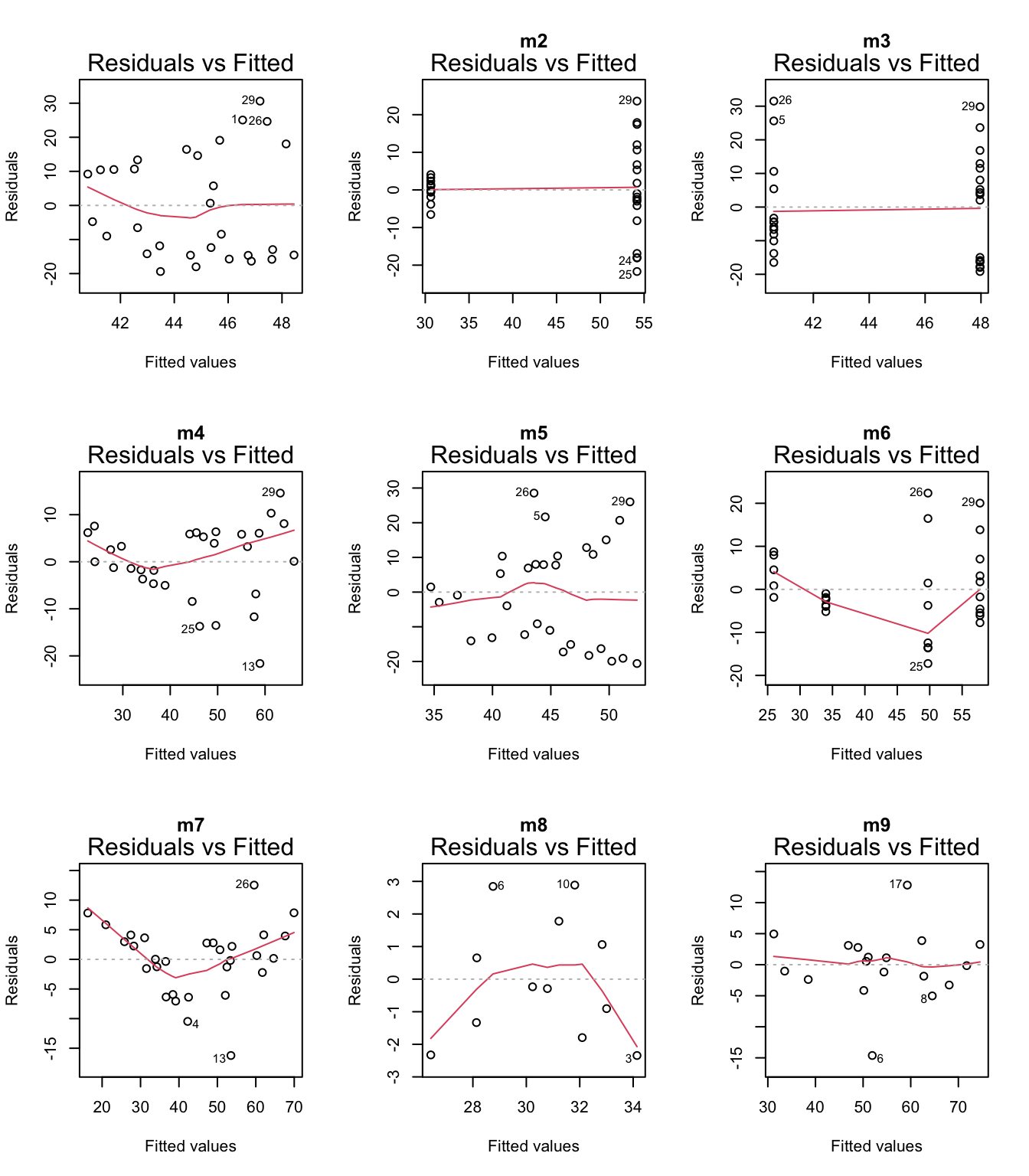

Version	Author	Date
dbfcd66	Paloma	2024-11-11

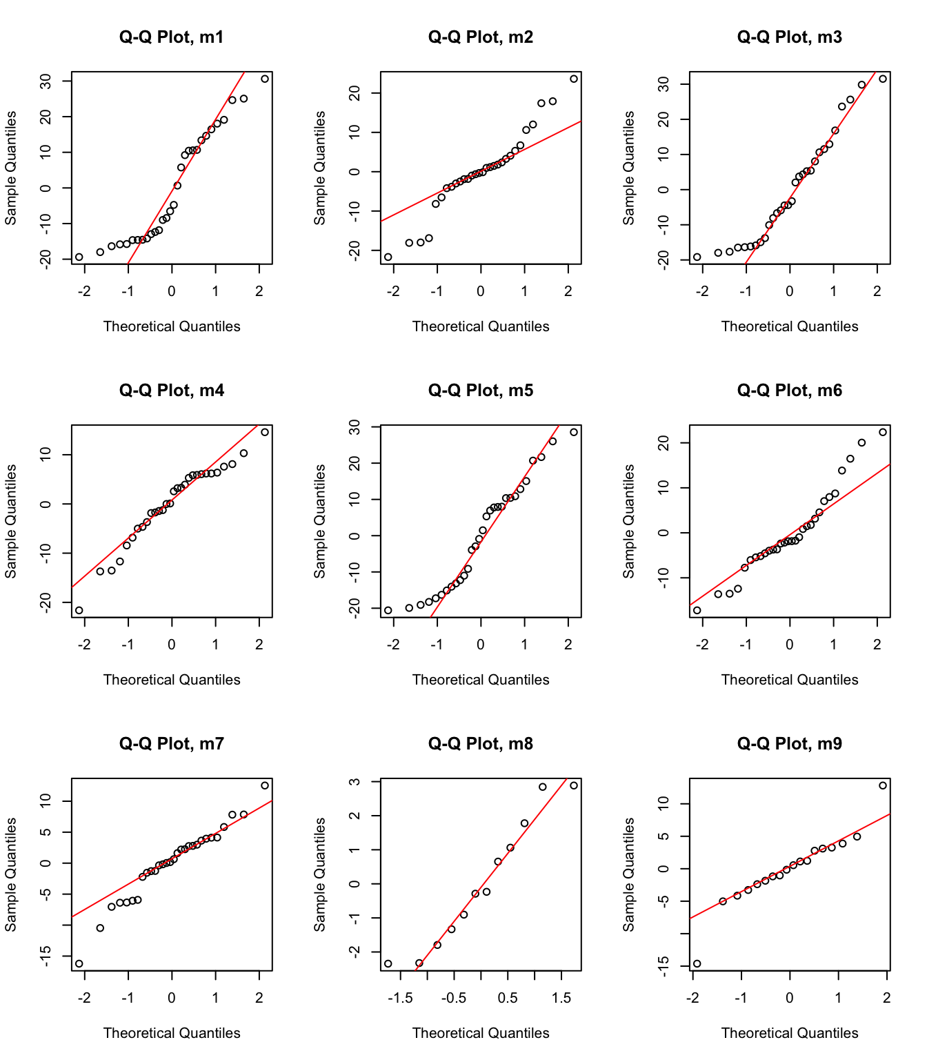
model <- list(m1, m2, m3, m4, m5, m6, m7, m8, m9)

par(mfrow = c(3, 3))

for (i in 1:length(model)) {
  # Create a Q-Q plot for the residuals of the i-th model
  qqnorm(residuals(model[[i]]), main = paste("Q-Q Plot, m", i, sep = ""))
  qqline(residuals(model[[i]]), col = "red")
}

Version	Author	Date
dbfcd66	Paloma	2024-11-11

Model 7 has the highest weight, a measure of certainty in the model. However, we need to consider that the distribution of the data is not normal. Perhaps I should try using other distributions (binom, posson, )

#scale variable

d2 <- data
d2$y <- data$Binding.Perc/100 

nll_beta <- function(mu, phi) {
  a <- mu * phi
  b <- (1 - mu) * phi
  -sum(dbeta(d2$y, a, b, log = TRUE))
}

# Fit models using mle2

fit <- mle2(nll_beta, start = list(mu = 0.5, phi = 1), data = d2)

Warning in dbeta(d2$y, a, b, log = TRUE): NaNs produced

Warning in dbeta(d2$y, a, b, log = TRUE): NaNs produced

Warning in dbeta(d2$y, a, b, log = TRUE): NaNs produced

Warning in dbeta(d2$y, a, b, log = TRUE): NaNs produced

Warning in dbeta(d2$y, a, b, log = TRUE): NaNs produced

summary(fit)

Maximum likelihood estimation

Call:
mle2(minuslogl = nll_beta, start = list(mu = 0.5, phi = 1), data = d2)

Coefficients:
     Estimate Std. Error z value     Pr(z)    
mu   0.450562   0.027216  16.555 < 2.2e-16 ***
phi 10.074474   2.483221   4.057  4.97e-05 ***
---
Signif. codes:  0 '***' 0.001 '**' 0.01 '*' 0.05 '.' 0.1 ' ' 1

-2 log L: -29.41959

m0n <- mle2(d2$y ~ dnorm(mean = a, sd = sd(d2$y)), start = list(a = mean(d2$y)), data = d2) 

# percent cover as predictor, use normal distribution
mcn <- mle2(d2$y ~ dnorm(mean = a + b * d2$Weight_mg, sd = sd(d2$y)), start = list(a = mean(d2$y), b = 0, s = sd(d2$y)), data = d2)

# scatter plot of 

plot(d2$y ~ d2$Weight_mg, 
     xlab = "Buffer",
     ylab = "% binding",
     col = "salmon",
     pch = 16, 
     las = 1)

#m0n
k <-coef(m0n)
curve(k[1] + 0 * x, 
      from = 0, to = 100, 
      add=T, lwd = 3, 
      col = "black")

#mcn
k <-coef(mcn)
curve(k[1] + k[2] * x, 
      from = 0, to = 100, 
      add=T, lwd = 2, 
      col = "lightgreen", 
      lty = "dashed")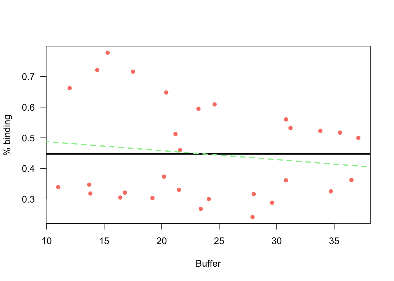

Version	Author	Date
dbfcd66	Paloma	2024-11-11

Finding optimal parameters using model 7

The goal is to run essays that result in a 50% binding.

# choose one model (m7: buffer + weight + spike)
coef <- coef(m7)

# Set target binding
target_binding <- 50

# FUNCTION to Solve for weight, assuming spike = 0
# 50% - intercept - (buffer1 * 1) - (spike * 0) / weight  

solve_for_weight <- function(dilution_value, spike_value = 0) {
  (target_binding - coef[1] - coef[3] * dilution_value - coef[4] * spike_value) / coef[2]
}

# Find the weight that gives 50% binding whenspike is 0
# dilution = 250
optimal_weight <- solve_for_weight(dilution_value = 1)
optimal_weight

(Intercept) 
   34.45251

# dilution = 60
optimal_weight <- solve_for_weight(dilution_value = 0)
optimal_weight

(Intercept) 
   23.58616

# Find the weight that gives 50% binding when spike is 1
# dilution = 250
optimal_weight <- solve_for_weight(dilution_value = 1, spike_value = 1)
optimal_weight

(Intercept) 
   6.377845

# dilution = 60
optimal_weight <- solve_for_weight(dilution_value = 0, spike_value = 1)
optimal_weight

(Intercept) 
  -4.488514

# visualize results
## Buffer = 1, Spike = 0
new_data <- expand.grid(weight = seq(min(weight), max(weight), length.out = 100),
                        buffer = as.factor(1), spike = as.factor(0))  # Set buffer and spike to a fixed value for simplicity

# Predict the binding percentage for the new data
new_data$predicted_binding <- predict(m7, newdata = new_data)

# Plot the predicted binding percentage against weight
ggplot(new_data, aes(x = weight, y = predicted_binding)) +
  geom_line() +
  geom_hline(yintercept = 50, linetype = "dashed", color = "red") +  # Highlight 50% binding
  labs(title = "Predicted Binding Percentage vs Weight (dilution = 60, spike = 1)",
       x = "Weight",
       y = "Predicted Binding Percentage")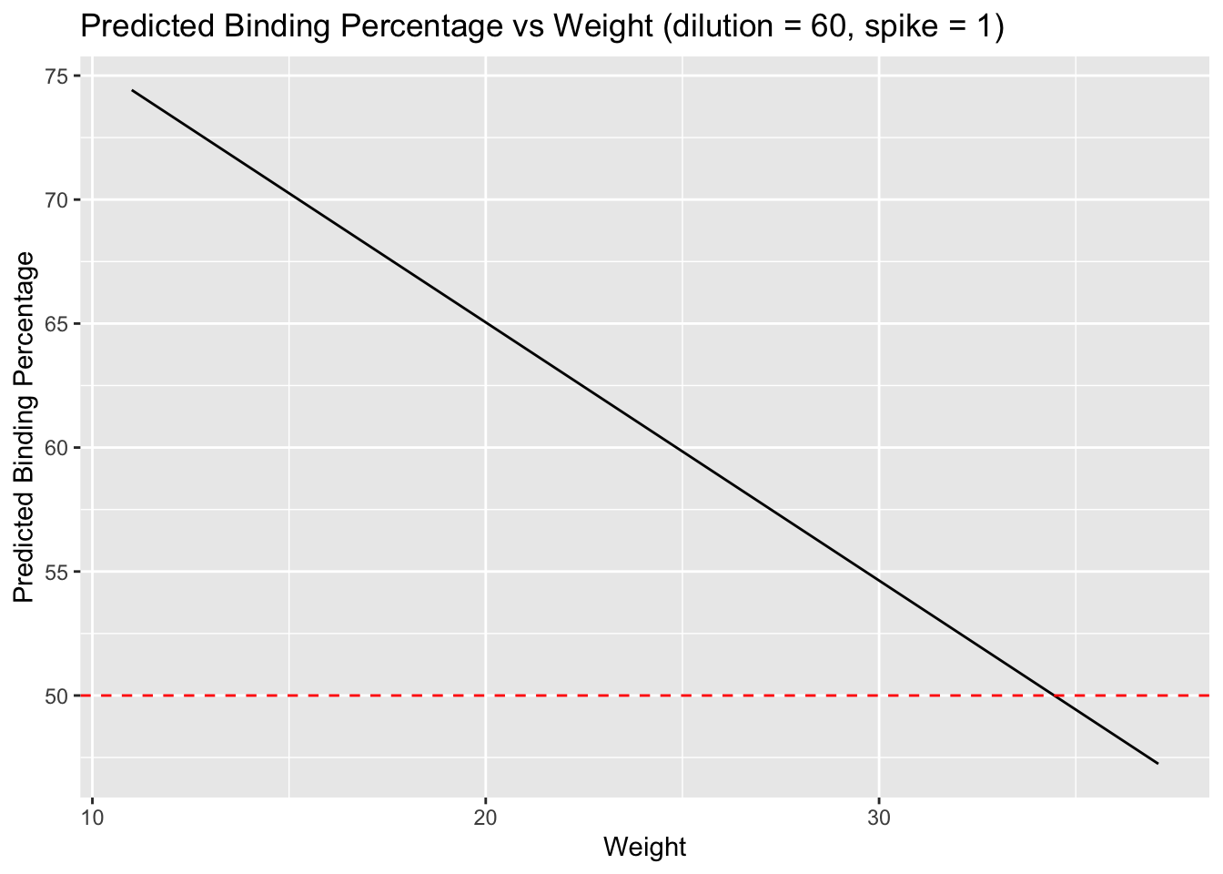

Version	Author	Date
dbfcd66	Paloma	2024-11-11

## Buffer = 1, Spike = 1
new_data <- expand.grid(weight = seq(min(weight), max(weight), length.out = 100),
                        buffer = as.factor(1), spike = as.factor(1))  # Set buffer and spike to a fixed value for simplicity

# Predict the binding percentage for the new data
new_data$predicted_binding <- predict(m7, newdata = new_data)

# Plot the predicted binding percentage against weight
ggplot(new_data, aes(x = weight, y = predicted_binding)) +
  geom_line() +
  geom_hline(yintercept = 50, linetype = "dashed", color = "red") +  # Highlight 50% binding
  labs(title = "Predicted Binding Percentage vs Weight (dilution = 250, spike = 1)",
       x = "Weight",
       y = "Predicted Binding Percentage")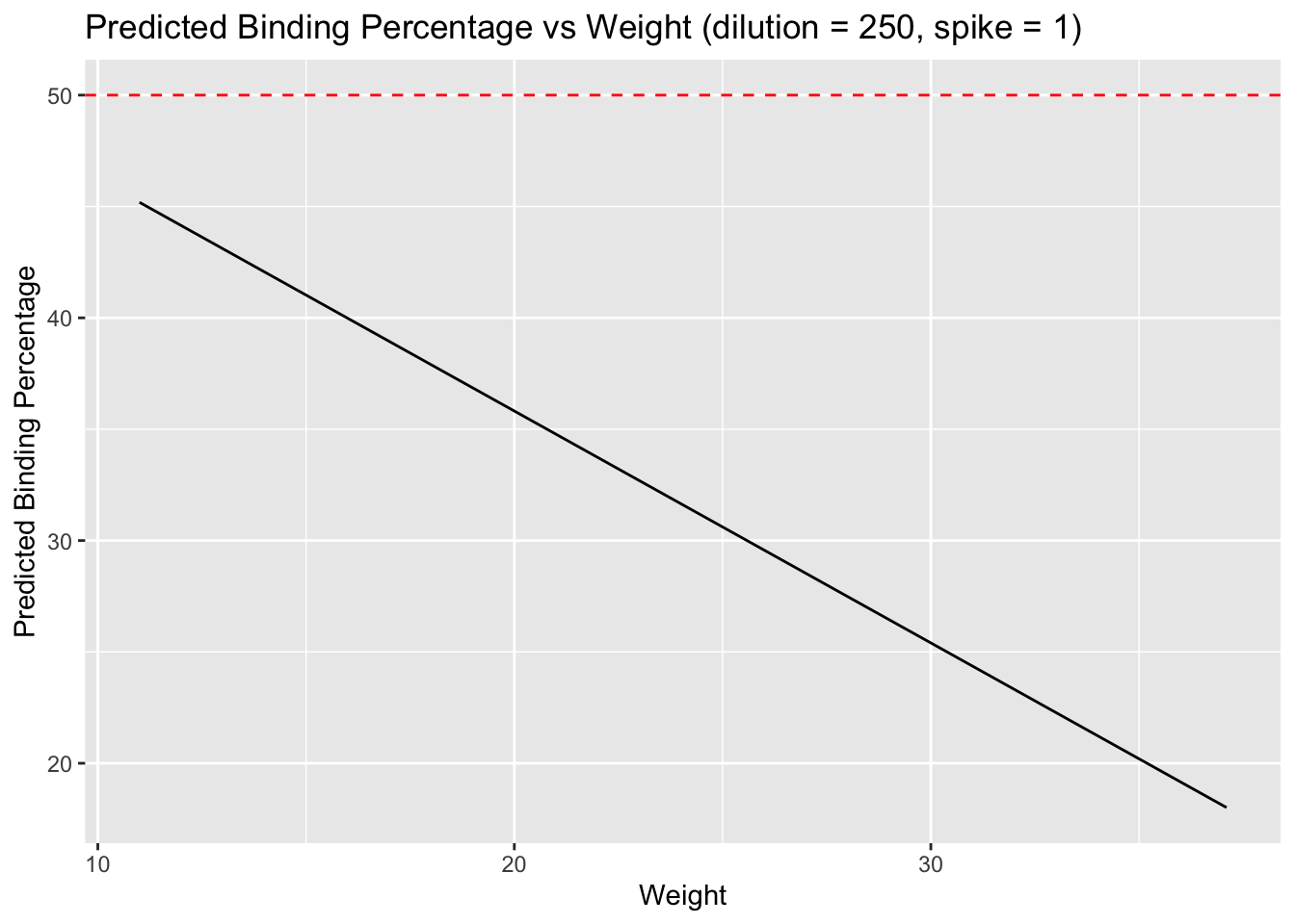

Version	Author	Date
dbfcd66	Paloma	2024-11-11

## Buffer = 0, Spike = 1

new_data <- expand.grid(weight = seq(min(weight), max(weight), length.out = 100),
                        buffer = as.factor(0), spike = as.factor(1))  # Set buffer and spike to a fixed value for simplicity

# Predict the binding percentage for the new data
new_data$predicted_binding <- predict(m7, newdata = new_data)

# Plot the predicted binding percentage against weight
ggplot(new_data, aes(x = weight, y = predicted_binding)) +
  geom_line() +
  geom_hline(yintercept = 50, linetype = "dashed", color = "red") +  # Highlight 50% binding
  labs(title = "Predicted Binding Percentage vs Weight (dilution = 250, spike = 0)",
       x = "Weight",
       y = "Predicted Binding Percentage")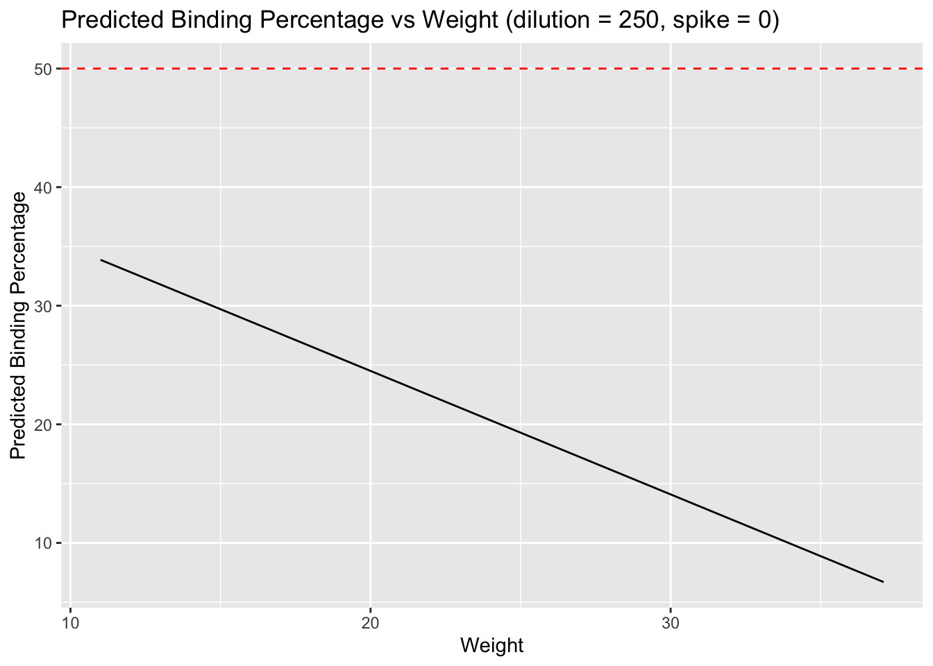

Version	Author	Date
dbfcd66	Paloma	2024-11-11

## Buffer = 0, Spike = 0

new_data <- expand.grid(weight = seq(min(weight), max(weight), length.out = 100),
                        buffer = as.factor(0), spike = as.factor(0))  # Set buffer and spike to a fixed value for simplicity

# Predict the binding percentage for the new data
new_data$predicted_binding <- predict(m7, newdata = new_data)

# Plot the predicted binding percentage against weight
ggplot(new_data, aes(x = weight, y = predicted_binding)) +
  geom_line() +
  geom_hline(yintercept = 50, linetype = "dashed", color = "red") +  # Highlight 50% binding
  labs(title = "Predicted Binding Percentage vs Weight (dilution = 60, spike = 0)",
       x = "Weight",
       y = "Predicted Binding Percentage")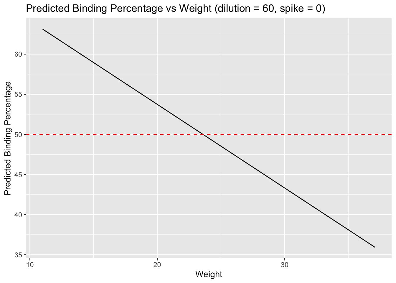

Version	Author	Date
dbfcd66	Paloma	2024-11-11

# FUNCTION to Solve for weight, assuming spike = 0
# 50% - intercept - (buffer1 * 1) - (spike * 0) / weight  

solve_for_weight <- function(dilution_value, spike_value = 0) {
  (target_binding - coef[1] - coef[3] * dilution_value - coef[4] * spike_value) / coef[2]
}


# Loop over different dilution values to find the optimal weight for 50% binding
# here, dilution 0 means 60uL, and 1 is 250 uL
for (buffer in seq(0, 1, by = 0.1)) {
  optimal_weight <- solve_for_weight(buffer)
  cat("Dilution:", buffer, "-> Optimal Weight for 50% Binding:", optimal_weight, "\n")
}

Dilution: 0 -> Optimal Weight for 50% Binding: 23.58616 
Dilution: 0.1 -> Optimal Weight for 50% Binding: 24.67279 
Dilution: 0.2 -> Optimal Weight for 50% Binding: 25.75943 
Dilution: 0.3 -> Optimal Weight for 50% Binding: 26.84606 
Dilution: 0.4 -> Optimal Weight for 50% Binding: 27.9327 
Dilution: 0.5 -> Optimal Weight for 50% Binding: 29.01933 
Dilution: 0.6 -> Optimal Weight for 50% Binding: 30.10597 
Dilution: 0.7 -> Optimal Weight for 50% Binding: 31.19261 
Dilution: 0.8 -> Optimal Weight for 50% Binding: 32.27924 
Dilution: 0.9 -> Optimal Weight for 50% Binding: 33.36588 
Dilution: 1 -> Optimal Weight for 50% Binding: 34.45251

sessionInfo()

R version 4.2.2 (2022-10-31)
Platform: aarch64-apple-darwin20 (64-bit)
Running under: macOS 15.0.1

Matrix products: default
BLAS:   /Library/Frameworks/R.framework/Versions/4.2-arm64/Resources/lib/libRblas.0.dylib
LAPACK: /Library/Frameworks/R.framework/Versions/4.2-arm64/Resources/lib/libRlapack.dylib

locale:
[1] en_US.UTF-8/en_US.UTF-8/en_US.UTF-8/C/en_US.UTF-8/en_US.UTF-8

attached base packages:
[1] stats4    stats     graphics  grDevices utils     datasets  methods  
[8] base     

other attached packages:
 [1] bbmle_1.0.25.1     arm_1.13-1         lme4_1.1-32        Matrix_1.5-4      
 [5] MASS_7.3-58.3      coefplot_1.2.8     RColorBrewer_1.1-3 ggplot2_3.4.2     
 [9] knitr_1.42         dplyr_1.1.2       

loaded via a namespace (and not attached):
 [1] Rcpp_1.0.10         bdsmatrix_1.3-6     mvtnorm_1.1-3      
 [4] lattice_0.21-8      rprojroot_2.0.3     digest_0.6.31      
 [7] utf8_1.2.3          R6_2.5.1            plyr_1.8.8         
[10] evaluate_0.20       coda_0.19-4         highr_0.10         
[13] pillar_1.9.0        rlang_1.1.0         rstudioapi_0.14    
[16] minqa_1.2.5         whisker_0.4.1       jquerylib_0.1.4    
[19] nloptr_2.0.3        rmarkdown_2.21      labeling_0.4.2     
[22] splines_4.2.2       stringr_1.5.0       useful_1.2.6.1     
[25] munsell_0.5.0       compiler_4.2.2      numDeriv_2016.8-1.1
[28] httpuv_1.6.9        xfun_0.39           pkgconfig_2.0.3    
[31] mgcv_1.8-42         htmltools_0.5.5     tidyselect_1.2.0   
[34] tibble_3.2.1        workflowr_1.7.0     fansi_1.0.4        
[37] withr_2.5.0         later_1.3.0         grid_4.2.2         
[40] nlme_3.1-162        jsonlite_1.8.4      gtable_0.3.3       
[43] lifecycle_1.0.3     git2r_0.32.0        magrittr_2.0.3     
[46] scales_1.2.1        cli_3.6.1           stringi_1.7.12     
[49] cachem_1.0.7        farver_2.1.1        reshape2_1.4.4     
[52] fs_1.6.1            promises_1.2.0.1    bslib_0.4.2        
[55] generics_0.1.3      vctrs_0.6.2         boot_1.3-28.1      
[58] tools_4.2.2         glue_1.6.2          abind_1.4-5        
[61] fastmap_1.1.1       yaml_2.3.7          colorspace_2.1-0   
[64] sass_0.4.5

Results

Paloma

2024-10-16

Introduction

Summary of results

Results

Binding percentages

Binding percentage by different variables

Value distributions by group (boxplots)

Coef. of variation percentage

Coef. of variation by group

Coef. of variation by different variables

Deviation from 50% binding

Analysis: linear models

Comparing models

Plot regression coefs

Plot model 1 to 4

Plot model 5 to 9

Summarize info multiple models

Comparing models using Akakike’s information criteria

Finding optimal parameters using model 7